Article

Radar Estimation of Intense Rainfall Rates through Adaptive Calibration of the Z-R Relation

1
Dipartimento di Ingegneria dell’Ambiente, del Territorio e delle Infrastrutture, Politecnico di Torino, Corso Duca degli Abruzzi, 24, 10129 Torino, Italy
2
Dipartimento Sistemi Previsionali, ARPA Piemonte, Via Pio VII, 9, 10135 Torino, Italy
*
Author to whom correspondence should be addressed.
Atmosphere 2015, 6(10), 1559-1577; https://doi.org/10.3390/atmos6101559
Submission received: 15 July 2015 / Revised: 29 September 2015 / Accepted: 14 October 2015 / Published: 22 October 2015
(This article belongs to the Special Issue Radar Meteorology)

Abstract

:
Rainfall intensity estimation from weather radar is still significantly uncertain, due to local anomalies, radar beam attenuation, inappropriate calibration of the radar reflectivity factor (Z) to rainfall rate (R) relationship, and sampling errors. The aim of this work is to revise the use of the power-law equation commonly adopted to relate radar reflectivity and rainfall rate to increase the estimation quality in the presence of intense rainfall rates. We introduce a quasi real-time procedure for an adaptive in space and time estimation of the Z-R relation. The procedure is applied in a comprehensive case study, which includes 16 severe rainfall events in the north-west of Italy. The study demonstrates that the technique outperforms the classical estimation methods for most of the analysed events. The determination coefficient improves by up to 30% and the bias values for stratiform events decreases by up to 80% of the values obtained with the classical, non-adaptive, Z-R relations. The proposed procedure therefore shows significant potential for operational uses.

1. Introduction

The use of weather radar to estimate rainfall rates and their spatio-temporal distribution is a well-established practice. Although the radar does not provide direct measures of rainfall fields, it is possible to estimate rainfall rates from the radar reflectivity measures. Weather radar provides spatial data with higher spatio-temporal resolution and lower maintenance costs than traditional rain gauging networks.
Rainfall rate and radar reflectivity are linked by the drop size distribution (DSD), as recognized by Marshall and Palmer [1]. The use of standard diameter distributions leads to a power law relation between the radar reflectivity factor Z ( mm 6 / m 3 ) and the rainfall rate R (mm/h):
Z = a · R b
where a and b are coefficients related to the DSD. In what follows, Equation (1) will be referred as the Z-R relationship and the “radar reflectivity factor” just as “reflectivity”.
As the Z-R relationship is inherently indeterminate, the coefficients a and b are usually estimated through an empirical approach, based on the comparison of radar and rain gauge data (e.g., [1,2]). The estimation procedure is characterized by a high level of uncertainty, as can be recognized by the wide variety of coefficient values collected in [3,4,5]. A variety of papers highlights the variability of a and b according to the type of event ([6,7]) and, during the event itself, in time and space ([8,9,10]). Even with measured drop size distributions, recorded over a physically homogeneous period, the instrumental noise related to small sampling effect and the observational noise, due to the drop sorting effect, can lead to Z-R relationships which are only true in a statistical sense [9].
Moreover, the expected estimation quality is considerably influenced by radar characteristics, sampling methodologies, and by the characteristics of the area in which the estimation is performed ([11,12,13]). The validity of an approach based on the use of a constant Z-R relationship should therefore be strictly limited to the calibration domain of the relation itself, making the relation unsuitable for any systematic operational use. The importance of distinguishing the search for a physical dependence between reflectivity and rainfall intensity in a specific context from the goal of obtaining the best radar estimation of the rainfall rate is well discussed in Ciach and Krajewski [14].
Optimal radar estimation of the rainfall rate, the main objective of this study, has been addressed by several papers in the literature. Some authors [15,16,17] propose to reduce the uncertainty of estimation by introducing additional information, e.g., type of precipitation, distance from the radar, etc.
Generally, a significant improvement in the estimation quality is obtained by calibrating Equation (1) at the local scale, on the rain gauge nodes. This kind of approach reduces the problems related to orographic and climatological spatial variability. Two main categories of methodologies can be adopted: (i) A long-term (static) approach that involves the calculation of a single corrective term from an historical dataset of radar and rainfall measurements, to be subsequently applied to all the time frames in an identical way; and (ii) a short-term (dynamic) approach which requires the definition of a different calibration factor for each time step, based on the comparison between radar and rain gauge data from a definite time domain [18]. Several studies can be found describing the results of the second category of methods, with approaches suitable for different time scales: seasonal (e.g., [19,20,21]), monthly (e.g., [22,23,24]), or multi-daily (e.g., [25]).
To adapt the estimation to a single event, different methodologies have been proposed, that can be referred to as assimilation techniques of radar and gauge information to derive bias-corrected precipitation fields. Most of them stem from the pioneering work of Brandes [26] that involves the computation of a calibration matrix for each event, based on the smoothing of both the original radar field and of the subsequent correction factors. The key idea of this work has been seminal for a wide range of radar adjustment methods accounting for the spatial variability of the a coefficient of the Z-R relation in an operative context (see e.g., [27]). As a conceptual evolution of the idea proposed in [26] recent methods propose adjustments of the relation (1) with Z-R data collected from moving windows at a sub-daily scale (e.g., [28,29]). More recent studies also report on the combination of this kind of approach with appropriate interpolation techniques to significantly increase the estimation quality [30].
Some authors ([31,32]) suggest another approach to increase the estimation quality, abandoning the classic radar-rain gauge comparison, and adopting different merging techniques, based on the use of geostatistical interpolators like kriging with external drift and co-kriging. More complex methodologies involve the use of advanced techniques such as statistical objective analysis [33] or Kalman filters (e.g., [34,35]). Most of these methods are very time consuming and often not suited to operational contexts [31].
Among the most recently proposed methods, the main advancement achieved in the operational efficiency relates to the use of non-linear calibration (i.e., methods which allow a and b to vary simultaneously). As demonstrated in various studies (e.g., [36]) those methods systematically outperform linear methods (where only the a coefficient is let to vary) due to the high variability of the b coefficient in time and space ([9,37]).
While most of the studies cited use either a spatial or a temporal point of view, we address the problem from both viewpoints at the same time, through a non-linear calibration procedure amenable to explain the variability of both the a and b coefficients simultaneously in space and time. We propose a simple and operationally-ready methodology that produces an accurate radar-based estimation of rainfall intensity, that is adaptive in time and independent of local conditions.
The quasi real-time calibration method proposed implies that Z-R relationships are consistent with the evolution of the event, while the use of a spatially adaptive approach avoids the use of interpolation techniques, making the technique amenable in large areas with complex orography. The aim is to make the methodology suitable for a systematic and unsupervised operational application.

2. The Adaptive in Time and Space Estimation Technique (ATS)

The proposed methodology aims to account for the spatio-temporal variability of the Z-R relation by means of an adaptive estimation of the two coefficients of Equation (1). The methodology, called Adaptive in Time and Space estimation technique (ATS) relies on the definition of calibration domains limited in time (Section 2.1) and space (Section 2.2).
In the following the rationale for the selection of the domains and the related calibration procedures in time and space are presented.

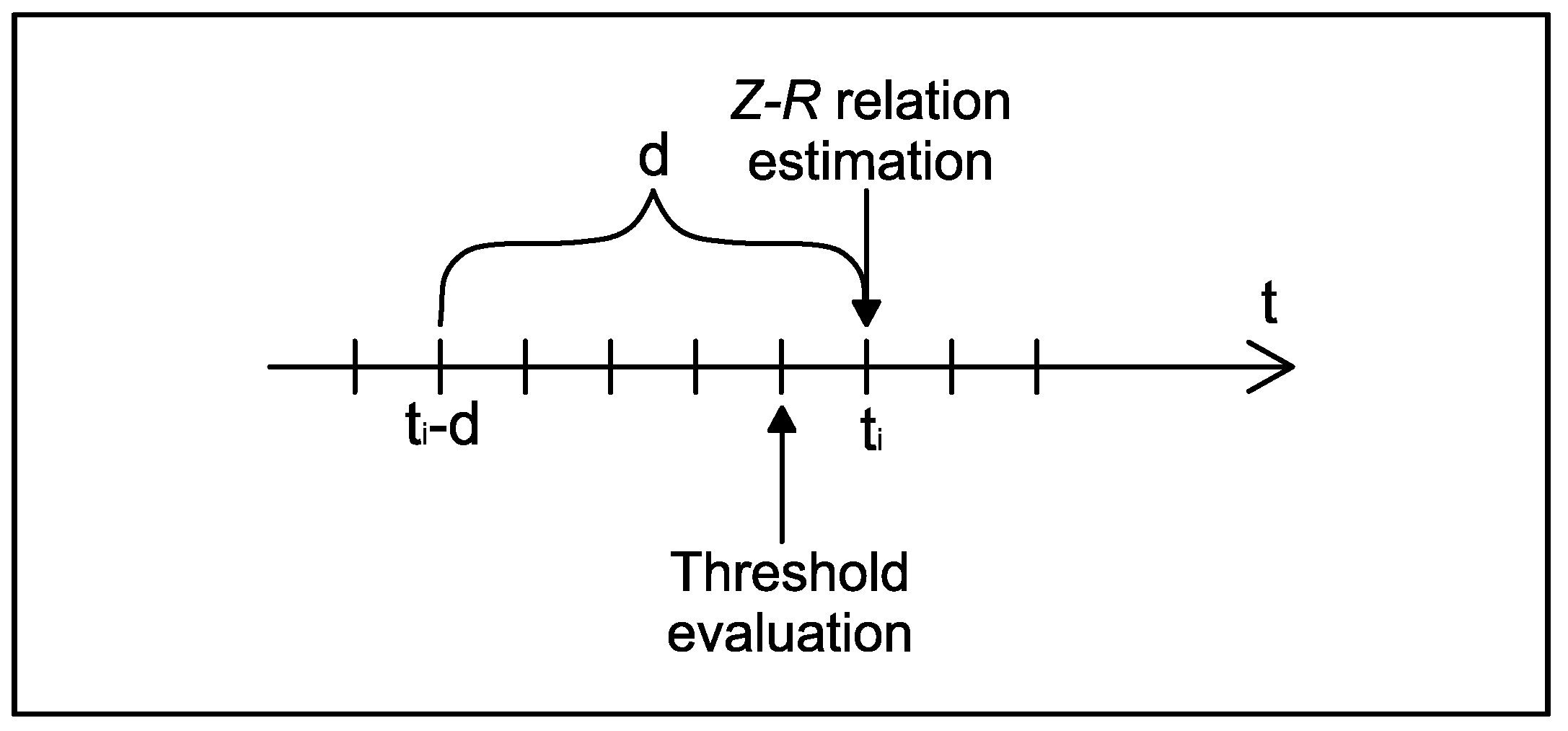
2.1. Definition of the Time Domain

To face the variability of the Z-R relation in time we propose to adopt a quasi real-time calibration window adapted from [29]: Coefficients a and b are estimated for each time step ( t i ) considering the Z-R pairs belonging to a calibration window of duration d, [ t i - d ; t i ], as shown in Figure 1.
Figure 1. Schematic representation of the temporal estimation domain.
Atmosphere 06 01559 g001
Such an approach allows one to follow the evolution of the event in quasi real-time, calibrating a different power-law relationship (1) at each time step. The inconvenience of this approach is that the high amount of noise can lead to highly variable estimates of the a and b coefficients due to the small size of the estimation domains.
To overcome this problem we propose a methodology involving a systematic “cleaning” of the data, using a reflectivity threshold variable in time to exclude from the estimation domain Z-R pairs with rainfall rate at or near zero. Working at a low rainfall rate scale, small differences between observed amounts and uncalibrated radar data can lead to spuriously large or small calibration factors [26]. Furthermore, the threshold is used to represents the amount of noise of the radar measurements due to instrumental and sampling uncertainly. The threshold is also used to discriminate between the presence and absence of rainfall at the considered time step: the rainfall rate is systematically set null for the locations characterized by under-threshold reflectivity values.
The threshold is calibrated for each t i by selecting the rain gauges that have registered no rainfall at the instant t i - 1 . The threshold value is defined as the quantile (with cumulative probability q) of the empirical distribution of the reflectivity data associated to the selected rain gauges. The choice of the optimal q value is discussed in Section 2.3.
After some preliminary test, we found that for a 10 minute resolution, a time window of 60 minutes provides sufficient information for a robust Z-R calibration. We decided not to let the width of the time window vary, to reduce the degrees of freedom of the procedure.

2.2. Definition of the Spatial Domains and Parameters Estimation

To account for the spatial variability of reflectivity, the calibration domain is further confined, for each location p j , to the N nearest rain gauges, using only above-threshold reflectivity values. In other words, for each pixel of the gridded study area, a specific calibration domain of N station is defined, N being therefore an important pre-determinate parameter in the procedure. The selection of the optimal N is widely discussed in Section 2.3. If the valid number of Z-R pairs (i.e., the above-threshold pairs into the whole estimation domain) are lesser than N, we attempt an estimation with the available pairs. If the number of Z-R pairs is not sufficient for a robust estimation (i.e., if the system does not converge after 400 iterations), a backup regional relationship is used (see Section 3.2 and Appendix A). Considering that the threshold value and the spatial distribution of rainfall change continuously, the procedure requires to re-consider the number and position of valid stations for each location p j at each time step t i .
Minimizing the sum of the squared differences between the observed and the estimated rainfall for each local domain and in each time step we obtain a pair of optimal a and b coefficients. The estimated rainfall R ^ is evaluated according to the following relationship, obtained from Equation (1), cleaning the recorded reflectivity with the threshold value Z t h :
R ^ = 10 Z * - Z t h * 10 · b ^ - l o g 10 a ^ b ^
where a ^ and b ^ are the estimated coefficients of the Z-R relationship, Z * (dBZ) and Z t h * (dBZ) the radar reflectivity and the reflectivity threshold respectively, both expressed in decibels ( Z * = 10 · l o g 10 Z ). As the definition of the local domains refers to the nearest rain gauge, local domains referred to near locations partially overlap one another, granting a smooth variation of the coefficients and the continuity of the radar QPE.
The estimation procedure is carried out in the Z-R plane by non-linear regression. The adopted optimization algorithm is a subspace trust region method and is based on the interior-reflective Newton method [38]. The optimized coefficients are estimated iteratively using as initial values the “static” coefficients calibrated at the regional scale (see Section 3.2). Calibration and verification procedures are carried out in cross-validation mode for each considered rain gauge, i.e., excluding one rain gauge at a time from the evaluation of the Z-R relationship and then comparing the estimated rainfall depth with the actual measurement at the excluded rain gauge.

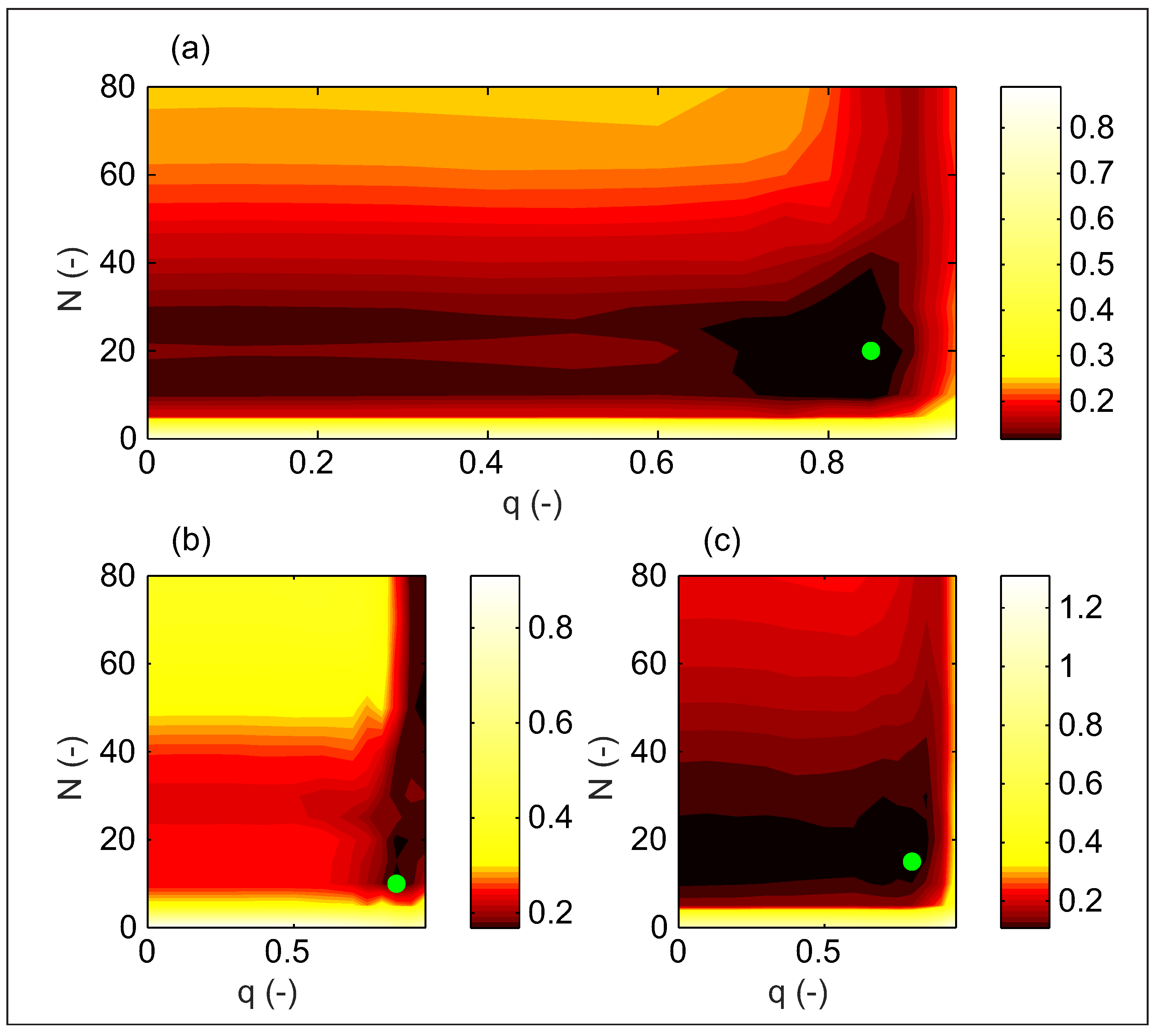
2.3. Calibration Procedure

The methodology is characterized by two calibration parameters: N and q, indicating the number of rain gauges in the local domain and the probability used for the definition of the zero-rainfall threshold respectively. First, we select an adequate number of severe precipitation events for the calibration. The rationale for the selection of the events is described in Section 3.2. On this dataset, in order to define the best N and q parameter values we proceed by maximizing the estimation efficiency at both hourly and event scale, considering jointly the absolute estimation error ε a b s , related to the hourly scale:
ε a b s = j = 1 n i = 1 d R ^ i , j - R i , j
and the BIAS, related to the event scale:
B I A S = 1 n j = 1 n i = 1 d ( R ^ i , j - R i , j )
where R i , j and R ^ i , j are the rainfall observed and estimated using Equation (1) respectively at t i in p j ; n is the number of rain gauges and d the number of records per rain gauge.
The calibration of N and q is therefore carried out by exploring the parameter space 0 q 0 . 9 and 0 N 80 (q=0 corresponding to the application of the methodology without any threshold) and minimizing the performance index I 3 , defined, for each event ( e v ), as:
I 3 , e v = I 1 , e v + I 2 , e v
where:
I 1 , e v = ε a b s m i n ( ε a b s ) - 1 · 100
and
I 2 , e v = B I A S m i n ( B I A S ) - 1 · 100
in which m i n ( ε a b s ) and m i n ( B I A S ) are the minima of ε a b s and BIAS, evaluated in the q-N parameter space. Optimal q and N are then chosen for each event as the values corresponding to the I 3 index minima.

3. Application

3.1. Case Study

The area of interest is located in North-Western Italy, almost entirely within the borders of the Piemonte region. The area is characterized by a complex orography as shown by Figure 2.
Figure 2. Orography of the study area and locations of “Bric della Croce” radar and rain gauge network.
Atmosphere 06 01559 g002
The presence of orographic barriers importantly affect radar detection quality, due to the presence of echoes from the ground, occlusions of radar beam, orographic precipitation under beam, etc. The “Bric della Croce” radar is a dual-polarization C-band doppler with digital receiver located at 736 m above sea level on the hills near Torino (Geographical coordinates: 7.734E 45.035N). ARPA Piemonte (the Regional Agency for Environmental Protection) stores reflectivity maps on a Cartesian grid of 250 × 250 km, with a resolution of 500 m in space and 10 minutes in time. The raw radar product is de-cluttered with a fuzzy logic algorithm [39] and the horizontal corrected reflectivity is projected on a 2D map by considering, at each point, the radar beam with lowest elevation available. This information is obtained comparing the terrain elevation for each cell of the gridded domain (extracted from a 500 × 500 m Digital Terrain Model) with the radar beam elevation. From October to May a VPR (Vertical Profile of Reflectivity) correction is applied. The mean VPR is calculated by averaging the vertical profiles falling into a neighbourhood with 50 km radius from the radar site, during the previous 1-hour period.
ARPA Piemonte also manages the rain gauge network, which consists of 378 tipping bucket gauges distributed over the Piemonte region (25,000 km 2 ). Rain data have a 10 minutes resolution in time and a minimum threshold of rainfall detection of 0.2 mm/10 min. This entails that the minimum intensity that a rain gauge can perceive is 12 mm/h. Intensity measures lower than 12 mm/h, with temporal resolution of 1 min, are hence the result of post-analysis algorithms [40].
As the aim of this work is the definition of an adaptive calibration method particular attention should be paid to the quality of input data.
The magnitude of the rain gauge errors is highly dependent on the local rainfall intensity and the timescale. For example, at moderate rainfall intensities of 10 mm/h [41] report relative standard errors of 4.9% for the 5-min and 2.9% for 15-min timescales. The available 10-minutes time resolution therefore results in a good compromise between relatively low standard errors and a good robustness at the hourly scale.
Much has already been said on the quality of the radar data in the previous sections. Supplementary analysis of the radar product quality, referred to the study case, is performed in Section 3.2, after the Selection of the events.

3.2. Definition of the Set of Events and Estimation of the Static Coefficients

The criteria that lead to the definition of the set of rainfall events to be used in this analysis comply with the need of representing the most intense precipitation events recently occurred in Piemonte. Two different categories of phenomena can be defined: (i) Convective events, typically very localized and characterized by high intensities and short durations, and (ii) stratiform events, covering wider areas and characterized by lower intensities and longer durations. We select the most intense events occurred in the region from 2003 to 2008, with different criteria for convective and stratiform events, based on the duration and spatial distribution of rainfall fields. Convective events are identified as those registering the annual maximum value (of hourly duration) in, at least, 22 rain gauges. Stratiform events, instead, are selected when the extension of the area registering the highest annual areal precipitation in 24/48 hours equals, at least, 1/4 of the regional area.
The selected events (18) are listed in Table 1.
Table 1. Dates and codes of the selected events.
IDConvective eventsIDStratiform events
127/07/2003931/10-01/11/2003
202/08/20051025/10-02/11/2004
320/08/20051115/04-17/04/2004
406/07/20061206/09-12/09/2005
512/07/20061314/09-15/09/2006
608/08/20071401/05-04/05/2007
730/08/20071525/05-28/05/2007
829/05/20081628/10-06/11/2008
1701/12-04/12/2003
1816/12-17/12/2008
In order to limit the amount of noise into the calibration procedure, we define the radar visibility map, to exclude the areas characterized by low quality reflectivity records, due to different source of errors (beam block, attenuation, etc.). To this aim we define the relation between the relative error at each gauged location and the beam height. A beam height of 4000 m a.s.l. is then used as threshold value to define the high visibility area, to be included in the calibration domain.
To further evaluate the quality of the used radar products we report in Table 2 the rate between invalid radar record at gauge location. Events 1 and 6 report anomalous high numbers of invalid radar records. We decided not to exclude the events from the case study to define the impact of these anomalies on the results.
Table 2. Number of invalid radar records divided by the total number of records for each event ( n i n v ).
EventninvEventninv
10.25490.001
20.003100.004
30.003110.005
40.004120.051
50.003130.003
60.461140.003
70.002150.073
80.050160.011
A backup version of Equation (1) is then calibrated over the high-visibility area to define a regional static (in time and space) relationship. This relation can be used as a backup-equation when the dynamic approach cannot be used. The regional calibration procedure, reported in the Appendix A, leads to the definition of the relationship (A1). Moreover, during the regional calibration phase, we decided to exclude events 17 and 18 from the case study, due to the probable presence of snow that could lead to mis-calibrations over the no-snowing areas (see the Appendix A for details).
Estimates obtained for the selected events with the regional relationship (A1) systematically outperform those obtained with commonly used relations (e.g., [2]). However, limitations due to the use of a single relation on a vast and complex territory, leading, in some cases, to poor reconstruction of the precipitation volumes are yet to be overcome. Figure 3 shows an example of the presence of over/underestimation clusters as a function of the distance of the location from the radar.
Figure 3. Comparison between observed precipitation R c u m and rainfall estimated with the regional formula R ^ c u m for the event occurred on 10/31-11/1/2003 at the event scale. (The grey scale refers to rain gauge distance from radar in km).
Atmosphere 06 01559 g003

3.3. Calibration of the ATS Technique

As stated in Section 2.1, the width d of the calibration window is set to one hour, in order to limit the influence of the temporal variability in the adaptive search for optimal parameter values. The use of Z-R data recorded with a 10 minutes frequency grants a good estimation robustness (5 samples for each window, each characterized by a number of observations equal to the number of considered rain gauges).
The adaptive calibration is carried out by evaluating, for each event, the pattern of the I 3 , e v index (Equation (5)) in the N-q parameter space. The minimization of this index allows to define the N-q pair that maximizes the estimation quality at both the hourly and the event scale.
The mean of the event patterns, each normalized to the maxima of I 3 , e v for the event, is plotted in Figure 4. The minimum of the I ¯ 3 index in the N-q parameter space identifies the optimal pair of values for the whole set of events. To evaluate the presence of different behaviours among the different event typologies, the calibration procedure is carried out at first on the whole set (Figure 4a), then on the convective ones (Figure 4b) and finally on the stratiform ones (Figure 4c).
For convective events, due to the high spatial variability of rainfall fields, a rather high q threshold is required, in order to exclude “false positive” values. The number of rain gauges in the local domain (N) seems to play a less important role, if a minimum of 5 rain gauges (corresponding to 25 Z-R pairs) is ensured. Below this value, the quality of the estimations rapidly declines, as shown in the panel (b) of Figure 4.
For stratiform events the number of rain gauges to be included in the domain becomes crucial and should be appropriately set (usually between 10 and 30) in order to avoid including in the estimation procedure stations with low information content. In this case the choice of the quantile q is less influential (see panel (c)), due to the low variability of the reflectivity values.
Table 3. Mean and standard deviation (Std) of the threshold values for the analysed events.
EventMean (dbZ)Std (dbZ)EventMean (dbZ)Std (dbZ)
1−2.066.51920.946.96
214.947.521011.7710.74
39.5510.701111.889.85
45.1711.51125.599.55
52.168.661316.737.99
62.589.97149.7810.38
74.459.54159.718.36
819.738.171617.706.30
Figure 4. Pattern of the I ¯ 3 index into the parameter space q-N (a) for all the selected events, (b) for convective only, (c) and for stratiform only events. q = 0 implies the application of the methodology without any threshold. The green dots indicate the location of the minima.
Atmosphere 06 01559 g004
We finally verify that the use of different N-q pairs for each category of events does not improve significantly the estimation quality. Therefore, in order to propose a methodology robust and easily applicable in real-time, we suggest to use as optimal values, both for convective and stratiform events, N = 20 and q = 85%, corresponding to the best global mean value of the I ¯ 3 index (Figure 4a).
These values are calibrated on the dataset under analysis but we are confident that they can be applied even in analogous spatial domains, whenever a local calibration can not be pursued. The limit of N = 20 in the spatial domain can grant a good robustness at the adopted time resolutions, and the relatively high quantile q for the definition of the threshold makes the methodology amenable to different kind of events. To support this statement, we show in Table 3 that the adopted quantile lets the threshold vary consistently even in our case study, without significant loss of performance with respect to the event-variable q values displayed by panels (b) and (c) of Figure 4.

4. Results and Discussion

The ATS procedure is applied to the 16 events listed in Table 1 using the q-N pair defined in the previous section. The performances of the procedure are compared with two static methodologies: the Joss-Waldvogel formula [2], routinely used for rainfall estimation over the study area, and the regional relation (Equation (A1)). We also compare our procedure with the adaptive methodology proposed by Brandes [26], that entails the estimation of a corrective factor at each rain gauge site, with a radar-gauge comparison carried out in real time. All factors are then interpolated on the whole radar field with the procedure described in [31]. Operatively, we adopt as first-attempt relation the regional one (Equation (A1)). To avoid the problems related to the low rainfall rate scale, we consider as valid only the pairs for which both recorded and estimated rainfall exceed 2.5 mm.
The quality indicators are defined at both the hourly and the event scale. Figure 5a,b show the coefficients of determination obtained with the four methodologies for all the events. Figure 5c shows the BIAS values.
The results confirm the validity of the proposed methodology that allows us to obtain lower volumetric errors for almost all of the events, with respect to both the static formulations. In addition, the correlation coefficients, not subjected to optimization during the calibration phase, show a general improvement in the estimation quality at both the hourly and the event scale.
As for the comparison with the adaptive methodology, the ATS technique shows remarkable improvements at the event scale, due to the contribution of the adaptive threshold to discriminate between presence and absence of rainfall, that leads to a more affordable estimation of the cumulative rainfall at the event scale. The improvement is greater for stratiform events, thanks to the spatial uniformity of these events, allowing an easier identification of the local spatial domains. For convective events the improvements are less marked, as the spatial variability of rainfall fields often leads the ATS technique to work as a regional estimator, similar to the one adopted in [26].
Events 1 and 6 are the only exceptions to the generally good performances. They are characterized by a generalized deterioration of the estimation quality, partly attributable to the poorer quality of the available data. The number of invalid radar record is indeed higher in events 1 and 6 than in all the other events, as reported in Table 2. This reduces the quality of results, as the efficiency of the proposed method, that involves a dynamic calibration, is quite sensitive to the quality of the input data.
To underline the validity of the proposed technique, in Figure 6 we compare the measured precipitation with the regional estimate (top graphs) and with the ATS estimate (bottom graphs) for 3 different events.
Graphs in column (a) and (b) show the comparison between the cumulative rainfall obtained with the regional relationship and the one obtained with the ATS technique, for the events 15 and 13, both considered at the event scale. The greater ability of the ATS technique to retrace the event is clearly apparent. The scatter plots in column (c) refer to the event 2, where data is aggregated at the hourly scale. In this case there is a deterioration of the determination coefficient, essentially due to the underestimation of a (limited) number of high values (that are underestimated also by the regional relationship).
Figure 5. Comparison between the coefficients of determination obtained with the Joss-Waldvogel formula, the regional formula, the methodology proposed in [26] and the ATS technique (a) at the event scale and (b) at the hourly scale. Correlation coefficient R 2 falling outside the range (0,1) have not been reported. (c) reports the comparison between the BIAS obtained with the four above-mentioned methodologies at the event scale.
Atmosphere 06 01559 g005
The results demonstrate that the proposed technique is particularly suitable for stratiform events. The wide spatial scale allows for an easy identification of the local spatial domain. Figure 6b shows the clearly improved estimation quality obtainable with the ATS technique with respect to a unique Z-R relation for a large-scale event.
The increase in the estimation quality is less significant for convective events, where the localized nature of the high values of reflectivity signal contrasts with the uneven spatial distribution of the rain gauges, preventing the identification of a uniform and numerically robust spatial domain. In these cases, to reach a sufficient number of representative station our procedure would require to use distant Z-R pairs, that can be poorly representative of the event core. Moreover, due to the rapid evolution in time, an hourly calibration window can be still too wide, leading to the use of non-representative Z-R pairs.
Given that the methodology has different performances for different spatial scales of the events, its validity for convective rainstorms needs to be further assessed. A more dense rain gauge network and the availability of radar-rainfall data with higher temporal resolution may facilitate the use of the adaptive approach, increasing the estimation quality, also for convective events.
Figure 6. Comparison between observed precipitation and rainfall estimated with the regional formula (top graphs) and with the ATS technique (bottom graphs). The comparison is made at the event scale for event 15 (column a) and 13 (column b). Comparison in (column c) refers to event 3 at the hourly scale. (The grey scale refers to the distance from radar, in km).
Atmosphere 06 01559 g006

5. Conclusions

A new, operationally oriented, procedure for the estimation of areal rainfall from weather radar is proposed. The methodology, called Adaptive in Time and Space (ATS), makes use of confined spatial and temporal domains for a quasi real-time calibration of the relation between radar reflectivity and rainfall rate at a local scale. By doing so we take into account the spatial and temporal variability of the Z-R relation, making the technique suitable for systematic operational use, regardless of local conditions, characteristics of the radar, sampling methodologies and spatio-temporal distribution of the events under analysis. The application of the ATS technique to a set of 16 severe rainfall events in the North-Western region of Italy provides a general improvement of rainfall estimation quality. A significant improvement in obtained particularly in the reconstruction of rainfall patterns of stratiform events from weather radar.
An accurate pre-processing of both radar and rainfall measurements is required in order to maximize the quality of the estimation. To make the methodology applicable in real-time, this operation has to be carried out in continuous time. This would require the implementation of automated procedures for evaluating the quality of input data and of output estimates, for immediate detection of anomalous values.
Further refinements to the proposed methodology are possible, such as varying the parameters of the calibration windows in time (e.g., time window amplitude, numbers of rain gauge into the local domain, percentile to be used to define the threshold), according to the evolution of the event. In order to make the procedure more robust and accurate, it could be also helpful to use multiple regression techniques during the calibration phase, by considering other radar variables (e.g., specific differential phase, differential reflectivity, etc.).
Future developments will address increasing the number of the events and the spatial domain, both to address the model performance deterioration for convective events and to test the validity of the ATS technique in different climatic areas, as well as to checking how different radar sampling methodologies (i.e., different beam height, different signal polarization, etc.) would affect the quality of the estimations.
All the data used in this study are freely available upon request from the corresponding author. CC BY-NC-ND

Acknowledgments

All the data used in this study are freely available upon request from the corresponding author. The authors wish to thank ARPA Piemonte for providing the data and in particular S. Barbero, and R. Bechini for useful technical discussions. Comments and suggestions by three anonymous reviewers are gratefully acknowledged. The work was partly funded by the Interreg-EU Project FLORA.

Author Contributions

P. Claps has outlined the guidelines of the study and has coordinated the different phases. F. Laio has conceived and designed the experimental phase and supervised the analysis of the results. P. Allamano and A. Libertino have managed the preliminary analysis of the data, and the experimental phase. R. Cremonini was involved in the supply and the pre-treatment of the data and offered technical support concerning the weather radar. A. Libertino wrote the paper.

Conflicts of Interest

The authors declare no conflict of interest.

A. Determination of a regional Z-R static relationship

In this appendix we briefly describe how we calibrate a static relation valid for the whole regional territory. To this aim, Equation (1) is reconsidered on the whole acceptance area in order to obtain regional estimates of the a and b coefficients. The calibration procedure is targeted at minimizing the absolute estimation error ε a b s (3) in the parameter space (1 < a < 1000, 1 < b < 4). In order to reduce the processing time, preliminary “data binning” was applied; i.e., radar reflectivity data were grouped into classes, with minimum width equal to the resolution of the radar data (0.5 dBZ). The median value was chosen as representative of each class. Classes with less than 10 items (i.e., the tails of the distribution) were assembled, to increase the robustness of the estimators. To each reflectivity class Z, a value of R equal to the average of the corresponding measured rainfall was associated.
Figure A1. (a) Ellipse of the absolute error (greyscale ellipses, mm) into the parameter space a - b . Grey dots represent the sub-minimum area; (b) Values of the BIAS (greyscale dots) and location of the minimum of the absolute error (+), of the BIAS (o) and of I 3 index (*) into the sub-minimum space for one of the selected events.
Atmosphere 06 01559 g007
Once identified the pair of parameters (a,b) characterized by the minimum standard deviation m i n ( ε a b s ) , the “sub-minimum area”, i.e., the area where the absolute error is at most twice of m i n ( ε a b s ) , is defined for each event (Figure A1a). The a-b calibration space is then limited to the “sub-minimum area”. On this domain we evaluate the BIAS for each a-b pair and for each event, according to Equation (4) (Figure A1b).
In order to define the optimal parameter pair, the absolute error ε a b s (3) and the BIAS (4) are combined for each event to define the index I 3 , e v (5). This index takes into account the quality of the estimation both at the hourly and event-scale.
We obtain the optimal pairs of a and b values, reported in Figure A2, by minimizing I 3 , e v for 8 convective and 10 stratiform events (see Table 1). Events 17 and 18, occurred in December 2003 and December 2008, are therefore excluded from the subsequent processing since they appear isolated from the others, probably due to the presence of snow. No distinction between convective and stratiform emerges from Figure A2.
The global optimal values of a and b are then obtained by applying the described procedure to the Z-R pairs of the whole set of events (i.e., merging convective and stratiform events).
The regional static relation reads:
Z = 40 · R ^ 2 . 5
where the (a,b) pair is represented by the big black dot in Figure A2.
Figure A2. Optimal (a-b) values of the Z-R relation for each single event (grey symbols, according to event type), for the different event categories (black rhombus and cross) and for the whole set of events (black dot).
Atmosphere 06 01559 g008

References

  1. Marshall, J.S.; Palmer, W.M.K. The distribution of raindrops with size. J. Metorol. 1948, 5, 165–166. [Google Scholar] [CrossRef]
  2. Joss, J.; Waldwogel, A. A method to improve the accuracy of radar-measured amounts of precipitation. In Proceedings of 14th Conference of Radar Meteorology, Tucson, AZ, USA, 17–20 November 1970; pp. 237–238.
  3. Battan, L. Radar Observation of the Atmosphere; University of Chicago Press: Chicago, IL, USA, 1973. [Google Scholar]
  4. Raghavan, S.S. Radar Metorology; Kluwer Academic Publisher: Dordrecht, The Netherlands, 2003. [Google Scholar]
  5. Doviak, R.J.; Zrnic, D.S. Doppler Radar and Weather Observations, 2 ed.; Dover Publication: Dover, UK, 2006. [Google Scholar]
  6. Tokay, A.; Short, D.A. Evidence from tropical raindrop spectra of the origin of rain from stratiform versus convective clouds. J. Appl. Meteorol. 1996, 35, 355–371. [Google Scholar] [CrossRef]
  7. Bringi, V.; Chandrasekar, V.; Hubbert, J.; Gorgucci, E.; Randeu, W.; Schoenhuber, M. Raindrop size distribution in different climatic regimes from disdrometer and dual-polarized radar analysis. J. Atmos. Sci. 2003, 60, 354–365. [Google Scholar] [CrossRef]
  8. Smith, J.A.; Krajewski, W.F. A modeling study of rainfall rate-reflectivity relationships. Water Resour. Res. 1993, 29, 2505–2514. [Google Scholar] [CrossRef]
  9. Lee, G.W.; Zawadzki, I. Variability of drop size distributions: Time-scale dependence of the variability and its effects on rain estimation. J. Appl. Meteorol. 2005, 44, 241–255. [Google Scholar] [CrossRef]
  10. Chapon, B.; Delrieu, G.; Gosset, M.; Boudevillain, B. Variability of rain drop size distribution and its effect on the Z-R relationship: A case study for intense Mediterranean rainfall. Atmos. Res. 2008, 87, 52–56. [Google Scholar]
  11. Cremonini, R.; Bechini, R. Heavy rainfall monitoring by polarimetric C-Band weather radars. Water 2010, 2, 838–848. [Google Scholar] [CrossRef]
  12. Krajewski, W.F.; Villarini, G.; Smith, J.A. RADAR-rainfall uncertainties where are we after thirty years of effort? Bull. Amer. Meteor. Soc. 2010, 91, 87–94. [Google Scholar] [CrossRef]
  13. Berne, A.; Krajewski, W.F. Radar for hydrology: Unfulfilled promise or unrecognized potential? Adv. Water Resour. 2013, 51, 357–366. [Google Scholar] [CrossRef]
  14. Ciach, G.J.; Krajewski, W.F. Radar-rain gauge comparisons under observational uncertainties. J. Appl. Meteorol. 1999, 38, 1519–1525. [Google Scholar] [CrossRef]
  15. Anagnostou, E.N.; Krajewski, W.F. Real-time radar rainfall estimation. Part I: Algorithm formulation. J. Atmos. Ocean. Technol. 1999, 16, 189–197. [Google Scholar] [CrossRef]
  16. Anagnostou, E.N.; Krajewski, W.F. Real-time radar rainfall estimation. Part II: Algorithm formulation. J. Atmos. Ocean. Technol. 1999, 16, 198–205. [Google Scholar] [CrossRef]
  17. Borga, M.; Anagnostou, E.N.; Frank, E. On the use of real-time radar rainfall estimates for flood prediction in mountainous basins. J. Geophys. Res.: Atmos. 2000, 105, 2269–2280. [Google Scholar] [CrossRef]
  18. Wood, S.; Jones, D.; Moore, R. Static and dynamic calibration of radar data for hydrological use. Hydrol. Earth Syst. Sci. Discuss. 2000, 4, 545–554. [Google Scholar] [CrossRef]
  19. Vieux, B.E.; Rendon, S.H. Derivation and Evaluation of Seasonally Specific Z-R Relationships; Final Report; South Florida Water Management District: West Palm Beach, FL, USA, 2009. [Google Scholar]
  20. Rendon, S.; Vieux, B.; Pathak, C. Estimation of regionally specific Z-R relationships for radar-based hydrologic prediction. In Proceedings of the World Environmental and Water Resources Congress, Providence, RI, USA, 16–20 May 2010; pp. 4668–4680.
  21. Pathak, C.; Teegavarapu, R. Utility of optimal reflectivity-rain rate (Z-R) relationships for improved precipitation estimates. In Proceedings of the World Environmental and Water Resources Congress, Providence, RI, USA, 16–20 May 2010; pp. 4681–4691.
  22. Seo, D.-J.; Breidenbacha, J.P.; Johnsonb, E.R. Real-time estimation of mean field bias in radar rainfall data. J. Hydrol. 1999, 223, 131–147. [Google Scholar] [CrossRef]
  23. Legates, D.R. Real-time calibration of radar precipitation estimates. Prof. Geogr. 2000, 52, 235–246. [Google Scholar] [CrossRef]
  24. Seo, D.J.; Breidenbach, J. Real-time correction of spatially nonuniform bias in radar rainfall data using rain gauge measurements. J. Hydrometeorol. 2002, 3, 93–111. [Google Scholar] [CrossRef]
  25. Rendon, S.; Vieux, B.; Pathak, C. Continuous forecasting and evaluation of derived Z-R relationships in a sparse rain gauge network using NEXRAD. J. Hydrol. Eng. 2013, 18, 175–182. [Google Scholar] [CrossRef]
  26. Brandes, E.A. Optimizing rainfall estimates with the aid of radar. J. Appl. Meteorol. 1975, 14, 1339–1345. [Google Scholar] [CrossRef]
  27. Nanding, N.; Rico-Ramirez, M.A.; Han, D. Comparison of different radar-raingauge rainfall merging techniques. J. Hydro. 2015, 17, 422–445. [Google Scholar] [CrossRef]
  28. Yufa, W.; Cuihong, W.; Hongxiang, J. Real-time synchronous integration of radar and raingauge measurements based on the quasi same-rain-volume sampling. Acta Meteor. Sinica 2010, 24, 340–353. [Google Scholar]
  29. Alfieri, L.; Claps, P.; Laio, F. Time-dependent ZR relationships for estimating rainfall fields from radar measurements. Nat. Hazard. Earth Syst. Sci. 2010, 10, 149–158. [Google Scholar] [CrossRef]
  30. Wang, G.; Liu, L.; Ding, Y. Improvement of radar quantitative precipitation estimation based on real-time adjustments to Z-R relationships and inverse distance weighting correction schemes. Adv. Atmos. Sci. 2012, 29, 575–584. [Google Scholar] [CrossRef]
  31. Goudenhoofdt, E.; Delobbe, L. Evaluation of radar-gauge merging methods for quantitative precipitation estimates. Hydrol. Earth Syst. Sci. 2009, 13, 195–203. [Google Scholar] [CrossRef]
  32. Velasco-Forero, C.A.; Sempere-Torres, D.; Cassiraga, E.F.; Jaime Gómez-Hernández, J. A non-parametric automatic blending methodology to estimate rainfall fields from rain gauge and radar data. Adv. Water Resour. 2009, 32, 986–1002. [Google Scholar] [CrossRef]
  33. Pereira, F.; Augusto, J. Improving WSR-88D hourly rainfall estimates. Weather Forecast. 1998, 13, 1016–1028. [Google Scholar] [CrossRef]
  34. Todini, E. A Bayesian technique for conditioning radar precipitation estimates to rain-gauge measurements. Hydrol. Earth Syst. Sci. 2001, 5, 187–199. [Google Scholar] [CrossRef]
  35. Chumchean, S.; Sharma, A.; Seed, A. An integrated approach to error correction for real-time radar-rainfall estimation. J. Atmos. Ocean. Technol. 2006, 23, 67–79. [Google Scholar] [CrossRef]
  36. Bruen, M.; O’Loughlin, F. Towards a nonlinear radar-gauge adjustment of radar via a piece-wise method. Meteorol. Appl. 2014, 21, 675–683. [Google Scholar] [CrossRef]
  37. Caracciolo, C.; Porcu, F.; Prodi, F. Precipitation classification at mid-latitudes in terms of drop size distribution parameters. Adv. Geosci. 2008, 16, 11–17. [Google Scholar] [CrossRef]
  38. Coleman, T.F.; Li, Y. An interior trust region approach for nonlinear minimization subject to bounds. SIAM J. Optim. 1996, 6, 418–445. [Google Scholar] [CrossRef]
  39. Davini, P.; Bechini, R.; Cremonini, R.; Cassardo, C. Radar-based analysis of convective storms over Northwestern Italy. Atmosphere 2011, 3, 33–58. [Google Scholar] [CrossRef]
  40. Habib, E.; Krajewski, W.F.; Kruger, A. Sampling errors of tipping-bucket rain gauge measurements. J. Hydrol. Eng. 2001, 6, 159–166. [Google Scholar] [CrossRef]
  41. Ciach, G.J. Local random errors in tipping-bucket rain gauge measurements. J. Atmos. Ocean. Technol. 2003, 20, 752–759. [Google Scholar] [CrossRef]

