Article

Meteorological Modeling Using the WRF-ARW Model for Grand Bay Intensive Studies of Atmospheric Mercury

1
Air Resources Laboratory, National Oceanic and Atmospheric Administration, 5830 University Research Court, College Park, MD 20740, USA
2
Cooperative Institute for Climate and Satellites, University of Maryland, 5825 University Research Court, College Park, MD 20740, USA
*
Author to whom correspondence should be addressed.
Atmosphere 2015, 6(3), 209-233; https://doi.org/10.3390/atmos6030209
Submission received: 29 September 2014 / Revised: 1 December 2014 / Accepted: 12 February 2015 / Published: 26 February 2015

Abstract

:
Measurements at the Grand Bay National Estuarine Research Reserve support a range of research activities aimed at improving the understanding of the atmospheric fate and transport of mercury. Routine monitoring was enhanced by two intensive measurement periods conducted at the site in summer 2010 and spring 2011. Detailed meteorological data are required to properly represent the weather conditions, to determine the transport and dispersion of plumes and to understand the wet and dry deposition of mercury. To describe the mesoscale features that might influence future plume calculations for mercury episodes during the Grand Bay Intensive campaigns, fine-resolution meteorological simulations using the Weather Research and Forecasting (WRF) model were conducted with various initialization and nudging configurations. The WRF simulations with nudging generated reasonable results in comparison with conventional observations in the region and measurements obtained at the Grand Bay site, including surface and sounding data. The grid nudging, together with observational nudging, had a positive effect on wind prediction. However, the nudging of mass fields (temperature and moisture) led to overestimates of precipitation, which may introduce significant inaccuracies if the data were to be used for subsequent atmospheric mercury modeling. The regional flow prediction was also influenced by the reanalysis data used to initialize the WRF simulations. Even with observational nudging, the summer case simulation results in the fine resolution domain inherited features of the reanalysis data, resulting in different regional wind patterns. By contrast, the spring intensive period showed less influence from the reanalysis data.

Graphical Abstract

1. Introduction

Mercury pollution remains a concern because of its effects on ecosystems, including threats to public health through fish consumption [1]. Atmospheric emissions and subsequent deposition are a significant pathway for mercury loading to ecosystems. It is therefore important to understand the sources of atmospheric mercury emissions, as well as its atmospheric fate and transport. The Great Lakes region has been one focus of study [2,3,4], while mercury pollution in the Gulf of Mexico region has also drawn increasing attention in recent years [5]. The observed atmospheric wet deposition flux of mercury in the Gulf of Mexico region is higher than that in any other region in the United States [6,7,8]. This is at least partly due to the relatively high rainfall rates in the region, as well as the higher prevalence of tall convective thunderstorms, resulting in the increased scavenging of free tropospheric mercury [9]. The Air Resources Laboratory (ARL) at the National Oceanic and Atmospheric Administration (NOAA) operates a station for the long-term monitoring of atmospheric mercury and other trace species at the Grand Bay National Estuarine Research Reserve (NERR) site in Moss Point, MS (30.412°N, 88.404°W). The station, located about 5 km from the Gulf, was one of the first such sites established in the National Atmospheric Deposition Program’s Atmospheric Mercury Network (AMNet). Measurements at the site support a range of research activities aimed at improving the understanding of the atmospheric fate and transport of mercury. Routine monitoring includes speciated Hg, ancillary chemical species and meteorological variables. Two intensive measurement periods were conducted at the site in summer 2010 and spring 2011 [8]. The atmospheric levels of gaseous oxidized mercury (GOM), the form of mercury that is most ecologically important, because it is readily deposited and is more bioavailable once deposited (e.g., most easily methylated), are highest in these two seasons.
Atmospheric models that simulate the fate and transport of emitted mercury can provide comprehensive source attribution information for a given region. The hybrid single-particle Lagrangian integrated trajectory (HYSPLIT) model [10] is a widely used trajectory and dispersion model for estimating source-receptor information on air pollutants. HYSPLIT back-trajectory analyses have been used in numerous atmospheric mercury studies [11,12,13]. In particular, a special version of the model (HYSPLIT-Hg), with an enhanced treatment of mercury chemistry and phase partitioning in the atmosphere, has been used to estimate detailed source-receptor relationships for atmospheric mercury deposition to the Great Lakes [2]. For such mercury modeling and for the comparable analysis of other pollutants, meteorological data are a critical input, as they control the transport and dispersion of pollutants, as well as the processes of wet and dry deposition. Atmospheric mercury is sensitive to the wind and temperature near the surface, as well as the planetary boundary layer (PBL) condition [14]. Hence, the quality of the meteorological data used influences the accuracy of the model results. The data should properly represent the spatio-temporal variations in the continuous fields of wind, temperature, precipitation, mixing and other relevant atmospheric properties. To better describe the mesoscale features in the region surrounding the NERR site during the measurement intensives, fine-resolution meteorological simulations were conducted by using the Weather Research and Forecasting (WRF) model [15] with data assimilation. As with any such model, errors will inherently exist in WRF-predicted fields due to the uncertainties associated with model dynamics, numerical algorithms, parameterization schemes, model initializations and input data. The inaccuracy of meteorological fields generated by the WRF model will be carried over to any pollutant fate and transport modeling using the data, resulting in errors in the estimates of source-receptor relationships. Thus, a comprehensive evaluation of WRF-generated meteorological fields is necessary before they are used to model the atmospheric transport and deposition of mercury.
To run the WRF model over a regional domain, reanalysis data, which are the results of other models (e.g., global reanalysis), are required to provide the initial conditions (IC) and lateral boundary conditions (LBC) for the simulations. Physical properties, such as momentum, heat and moisture, from the reanalysis data provide the initial state of the atmosphere in the regional domain and constrain the development of weather systems within time-varying lateral boundaries. However, biases in the IC/LBC data can affect the accuracy of the regional simulation results in dynamic downscaling [16]. There is no consensus about which reanalysis data provide the best IC/LBC for regional simulations. IC/LBC data with higher temporal and/or spatial resolution may not necessarily lead to better regional modeling results. The choice of IC/LBC data for the regional model can thus significantly influence the prediction of regional wind patterns, even in the finest resolution domain of a three-nested-domain configuration [17]. Thus, WRF performance must be assessed by using alternative IC/LBC inputs.
For reducing model bias during the simulation, four-dimensional data assimilation (FDDA), or nudging, is a well-known and efficient method available in the WRF model [18]. This approach adjusts model values toward observations (observational nudging) or toward analysis fields (grid or analysis nudging) for temperature, moisture and the u- and v-components of wind at each integration time step. Furthermore, Deng et al. [18] also suggested that in order to provide more accurate IC/LBC data for the regional modeling, reanalysis data must undertake an objective analysis process with surface and upper level meteorological data before being used to initialize the WRF model. Studies [17,19,20,21,22,23] have demonstrated that nudged results outperform simulations without nudging, which is also beneficial for air quality applications, including chemical and dispersion modeling. However, there are different suggestions for configuring the nudging process in order to minimize model bias, and the situation is complex, as physics schemes for the surface and PBL develop their own local-scale dynamics regardless of the influence of “artificial” nudging. Grid nudging of wind within the PBL (including the surface layer) is the preferred protocol of the U.S. EPA for retrospective meteorological simulations used in air quality studies [24]. Rogers et al. [22] presented sensitivity tests for nudging configurations and found that multiscale FDDA combining both analysis and observational nudging produced the smallest errors. Hegarty et al. [23] found that grid nudging within the PBL corrected an overestimate in plume transport possibly caused by a positive surface wind bias in WRF. Godowitch et al. [21] showed that eliminating nudging within the surface layer and PBL resulted in a better prediction of nocturnal jet speed. Gilliam et al. [24] suggested that the use of the wind profile aloft without surface nudging improved modeled winds within the convective PBL and above the stable PBL at night.
The overall goal of this study is to find a suitable WRF-model configuration to develop a high-quality, high-resolution regional- and local-scale meteorological dataset to support mercury modeling for the two measurement campaigns at the Grand Bay station conducted in summer 2010 and spring 2011. We evaluate the WRF model performance through comparison with observations, including surface measurements and soundings at the Grand Bay NERR station. WRF simulations are generated by using different reanalysis data for IC/LBC to examine influences on the prediction of regional flows in the WRF model. Another set of WRF simulations is conducted to examine the effect of the nudging strategy on model performance. Through the evaluation of meteorological model results, we may be able to identify the inaccuracy in meteorological data affecting the simulation of pollutant transport. Section 2 describes the model configuration for WRF, experiment designs (i.e., the WRF model configurations) for the different sets of simulations carried out, sources of observation, model evaluation methodology and the HYSPLIT model used for the backward trajectory analysis, as well as reviews the two Grand Bay Intensive campaigns, including synoptic weather and mercury episodes. In Section 3, the model results and analyses are presented for the summer and spring campaigns. Our conclusions are presented in Section 4.

2. Experimental Section

2.1. Configuration of the WRF Model

The Advanced Research WRF version 3.2 is used to simulate weather conditions during two Grand Bay Intensive measurement periods in summer 2010 (28 July to 15 August) and spring 2011 (19 April to 9 May). The modeling domains (Figure 1) include three nested grids with 36-km resolution (D01) for the contiguous U.S., 12-km resolution (D02) for the Eastern U.S. and 4-km resolution (D03) for the Gulf Coast of Louisiana, Mississippi and Alabama. Altogether, 43 vertical sigma layers are used, with the higher resolution near the ground to better describe the atmospheric structure in the lower boundary layer. The thickness of the lowest layer is around 34, and 15 layers are included below 850 hPa ( 1.5 km). The two coarser domains are run with two-way nesting, while the finest domain (D03) is initialized by using the D02 result. The physics options include the rapid radiative transfer model for longwave radiation [25], the Dudhia scheme for shortwave radiation [26], the Pleim–Xiu land surface model [27,28], the Asymmetrical Convective Model 2 for PBL parameterization [29], WSM3 for microphysics [26] and the Grell–Devenyi Ensemble [30] for the sub-grid cloud scheme.

2.2. WRF Simulation Designs

2.2.1. Reanalysis Data for WRF Model Initialization

To initialize the WRF model for the North American regional domain, either reanalysis data or global model products can provide the required meteorological fields for IC/LBC. Four reanalysis products are used to initialize the WRF simulations for the Grand Bay Intensive period of summer 2010: (1) the National Centers for Environmental Prediction (NCEP) North American Regional Reanalysis (NARR) at 32-km resolution with 29 pressure levels [31]; (2) the NCEP Global Final Analysis with data assimilation from the Global Forecast System (GFS) in 1 × 1 degree spacing and 26 vertical layers [32]; (3) the NCEP-National Center for Atmospheric Research Reanalysis Product (NNRP) in a 2.5 degree latitude-longitude grid with 17 pressure levels and 28 sigma levels [33]; and (4) the NCEP Climate Forecast System Reanalysis (CFSR) at 38-km spatial resolution and 64 pressure levels [34]. They are all available at 6-h intervals; except NARR, which is 3 hourly. We evaluate the results of the WRF modeling run by using the same model configuration (detail shown in Section 2.1), but with the four sources of IC/LBC data above.
Figure 1. The three nested domains for WRF simulations and observation stations used in this study.
Atmosphere 06 00209 g001

2.2.2. Nudging Procedure

The practice of objective analysis together with grid and observational nudging in meteorological modeling has been shown to be beneficial in generating inputs for air quality studies. Objective analysis modifies the first guess (i.e., reanalysis data) by ingesting information from given observations to provide more accurate IC/LBC data for WRF initialization. Objectively analyzed data also provide analysis fields for the grid nudging of wind, temperature and moisture to constrain the error growth during the simulation. In this study, the surface, sounding and wind profiler data obtained from the Meteorological Assimilation Data Ingest System (MADIS) are ingested in the simulations through objective analysis and nudging to maintain the model results close to the given observations. The Grand Bay measurements and the Soil Climate Analysis Network (SCAN) data are not included in the objective analysis and nudging, but rather reserved as an independent dataset for the model evaluation. Grid nudging and/or observational nudging are applied for all of the domains throughout the simulations to minimize errors. Three WRF simulations with different nudging configurations are conducted for the summer 2010 campaign: (1) allDA, grid nudging (including surface) and observational nudging of all fields, temperature, moisture and the u- and v-components of wind; (2) wdDAno3D, observational nudging of wind components, but no grid nudging; and (3) wdDA, grid nudging (including surface) and the observational nudging of wind fields.

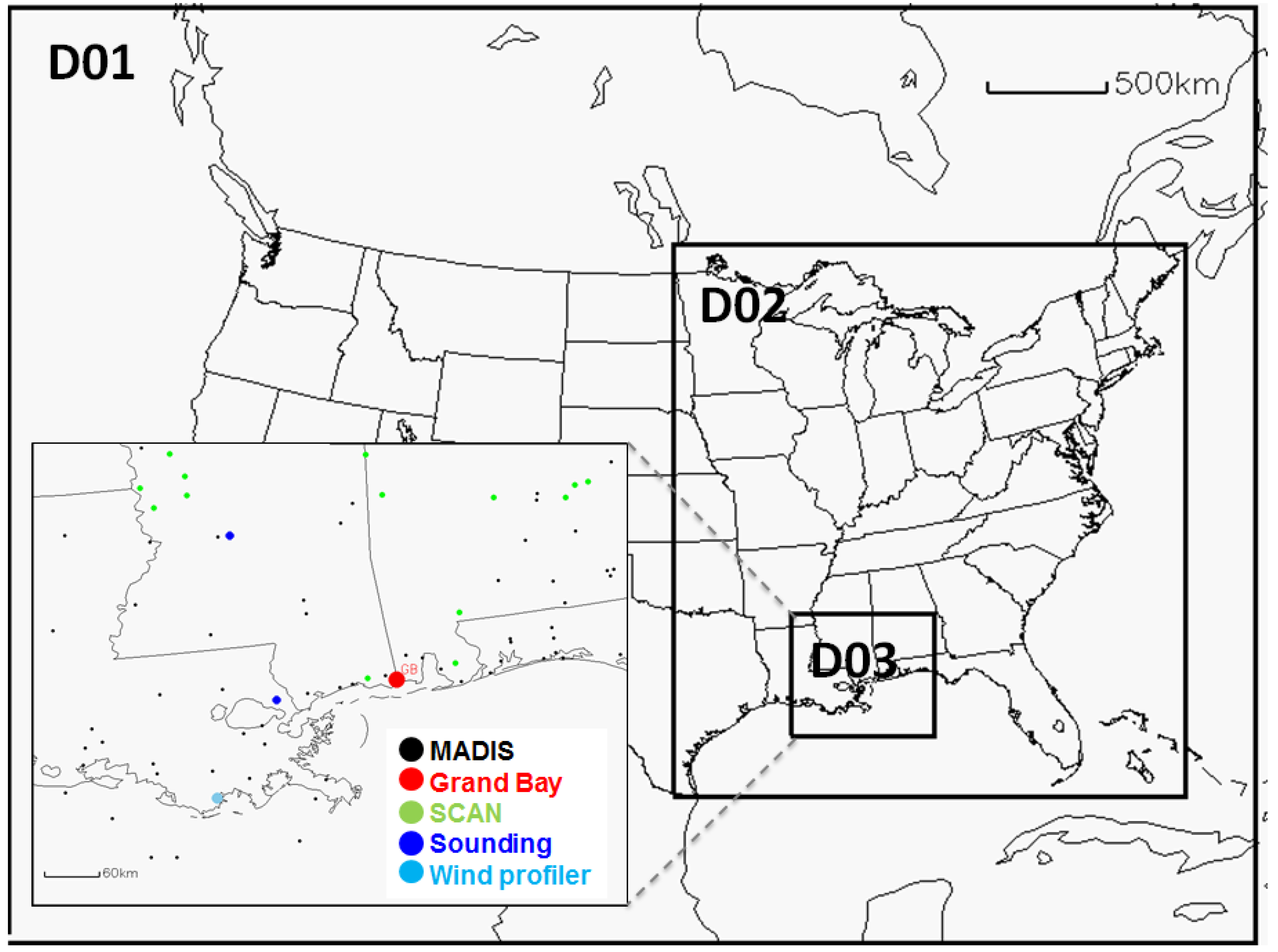
2.3. Observation Data for Model Evaluations

The locations of observation data used in the analysis are shown in Figure 1. This study uses meteorological measurements from three sources: (1) The Grand Bay NERR site provides surface meteorological measurements and extra soundings launched during the intensive period. Details on the Grand Bay station and measurements taken during the two campaigns are contained in [8]. (2) The MADIS (http://madis.noaa.gov/) developed by the NOAA Earth System Research Laboratory collects observations from a wide range of national and international data sources, and its data are integrated and quality controlled. Relevant surface and upper level (sounding and wind profiler) observations are downloaded and extracted for the study domains. (3) The SCAN (http://www.wcc.nrcs.usda.gov/scan) operated by the Natural Resources Conservation Service provides regular meteorological observations, including temperature, relative humidity, pressure, wind speed and wind direction. Two SCAN sites are relatively close to the Grand Bay station, while the rest are inland.
The evaluation of WRF results focuses on the 4-km domain (D03) for wind speed, wind direction, temperature and relative humidity. Gridded model values are paired with corresponding observations in space and in time for the comparison. If a missing data point was encountered, the station at that particular time step would be skipped. To assess the model performance, we provided domain-wide statistics calculated with simulated and measured values. a combination of metrics is suggested for model evaluations, since a single statistical metric only provides a limited characterization of the errors [35]. Statistical summaries include: the correlation coefficient (R) describing the extent of the linear relationship between the model and observed values; the mean absolute error (MAE) and root mean square error (RMSE), together with mean bias (bias), summarizing how close the predicted values are to the measured values; the standard deviation of the error (SDE), measuring the amount of variation from the average error; Index of Agreement (IOA), indicating how well the model represents the pattern of perturbation about a mean value. These statistical measures are commonly used for evaluations of meteorological and air quality models ([20,36,37], etc.), and a more detailed description of them can be found in [38].

2.4. Backward Trajectory Analysis

The ultimate use of the WRF fine-resolution meteorological results is to support the trajectory and dispersion analysis of atmospheric mercury in the Grand Bay region. The HYSPLIT model is used to understand how different meteorological inputs affect the estimates of source-receptor relationships. The model is designed for both simple air parcel trajectories and complex dispersion and deposition simulations. It has been used for trajectory analysis to identify the source-receptor relationships of air pollutants and for dispersion predictions for a variety of events, such as nuclear incidents, volcanic eruptions, wild fire smoke transport and dust storm episodes (http://ready.arl.noaa.gov/index.php). Backward trajectories are computed for particular mercury episodes during the intensive period utilizing WRF meteorology conducted with different model configurations, as described in the previous sections. Trajectory analysis can be a useful assessment tool for selecting more accurate WRF meteorology and estimating meteorological uncertainty, because the trajectories represent the space- and time-integrations of the velocity fields rather than just relying on verification statistics at fixed locations.

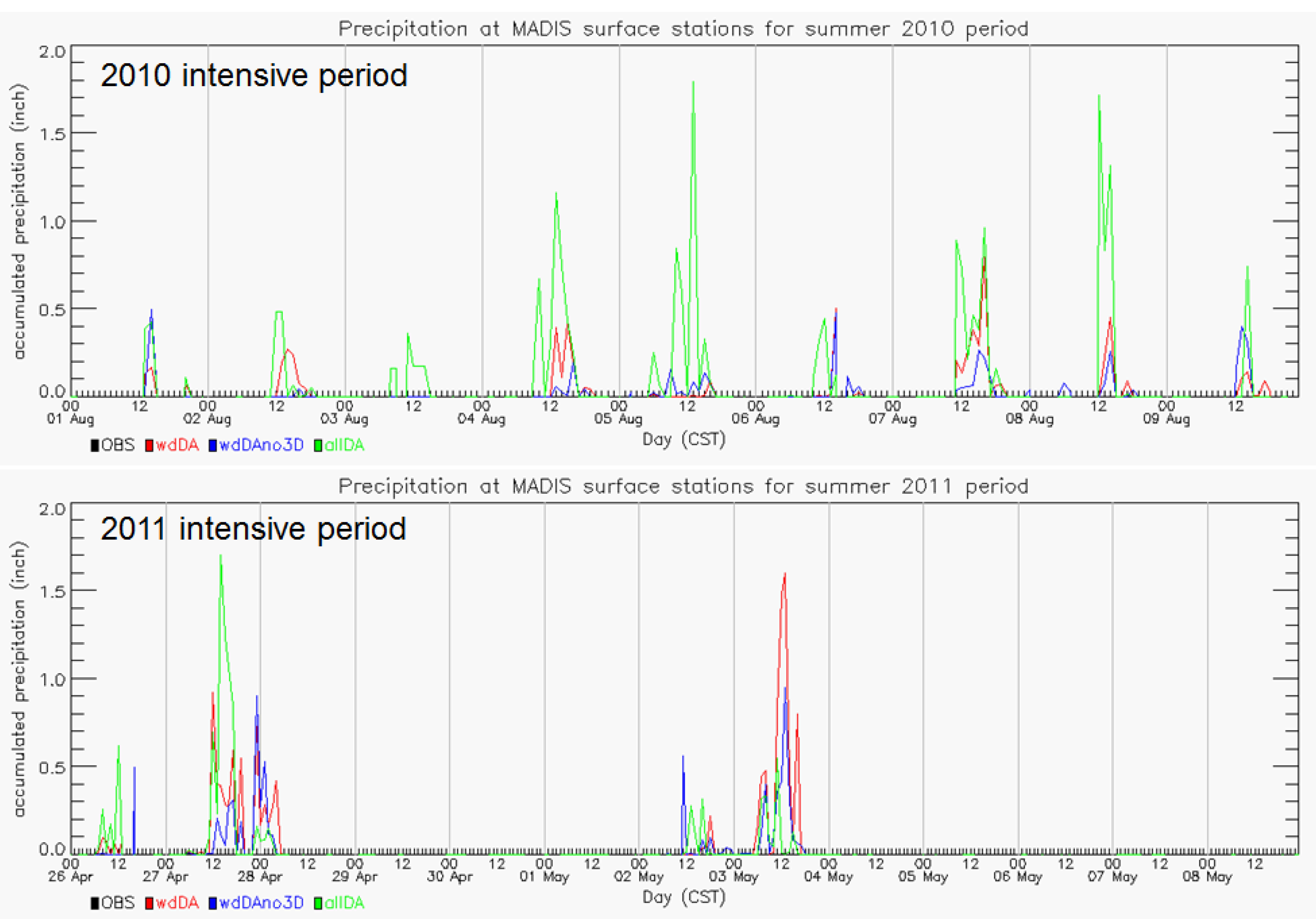
2.5. Overview of Grand Bay Intensive Measurements Periods

For the Grand Bay Intensive measurement in summer 2010 (28 July to 15 August) a high pressure system was dominant in the Gulf at the beginning of the study period. The system was weakening, and a weak stationary front was approaching the coast of Mississippi on 2 August. During this period, the ambient temperature was around 33 °C as the daytime maximum and 25 °C as the nighttime minimum, while the wind speed was light to moderate with a mostly southerly to southwesterly flow. Gaseous oxidized mercury (GOM) mid-day peaks of 20–60 pg/m3 were observed at Grand Bay on 2, 4–7 August (indicated in Figure 2, top panel), while the typical peak value ranged about 10–20 pg/m3. The average gaseous elemental mercury (GEM) level of the campaign period was 1.42 ng/m3 [8]. Another stationary front approached the Grand Bay site on 7 and 8 August. Moisture-rich Gulf air interacting with the approaching stationary front led to thunderstorm development, and a significant amount of rainfall was measured at Grand Bay during this period.
Another Grand Bay Intensive period was conducted from mid-April to mid-May 2011 (19 April to 9 May). During the first 9 days, frontal activities were confined largely to the north of the Grand Bay region, and the area was dominated by southerly flows. On 28 April and 3 May, cold fronts passed through the area, bringing continental cold air masses to the station. After these frontal passages, the area experienced post-frontal conditions, namely dry air, low night-time temperatures (as low as 10 °C), a light northeasterly wind in the morning and a southerly sea breeze in the afternoon. Wind speed was moderate in general, but became gradually smaller after the second frontal passage on 3 May. Mercury episodes were identified on 29 April and 4–7 May (indicated in Figure 7, top panel), as high levels of GOM were observed at the Grand Bay site with peak values of 30–70 pg/m3 [8].

3. Results and Discussion

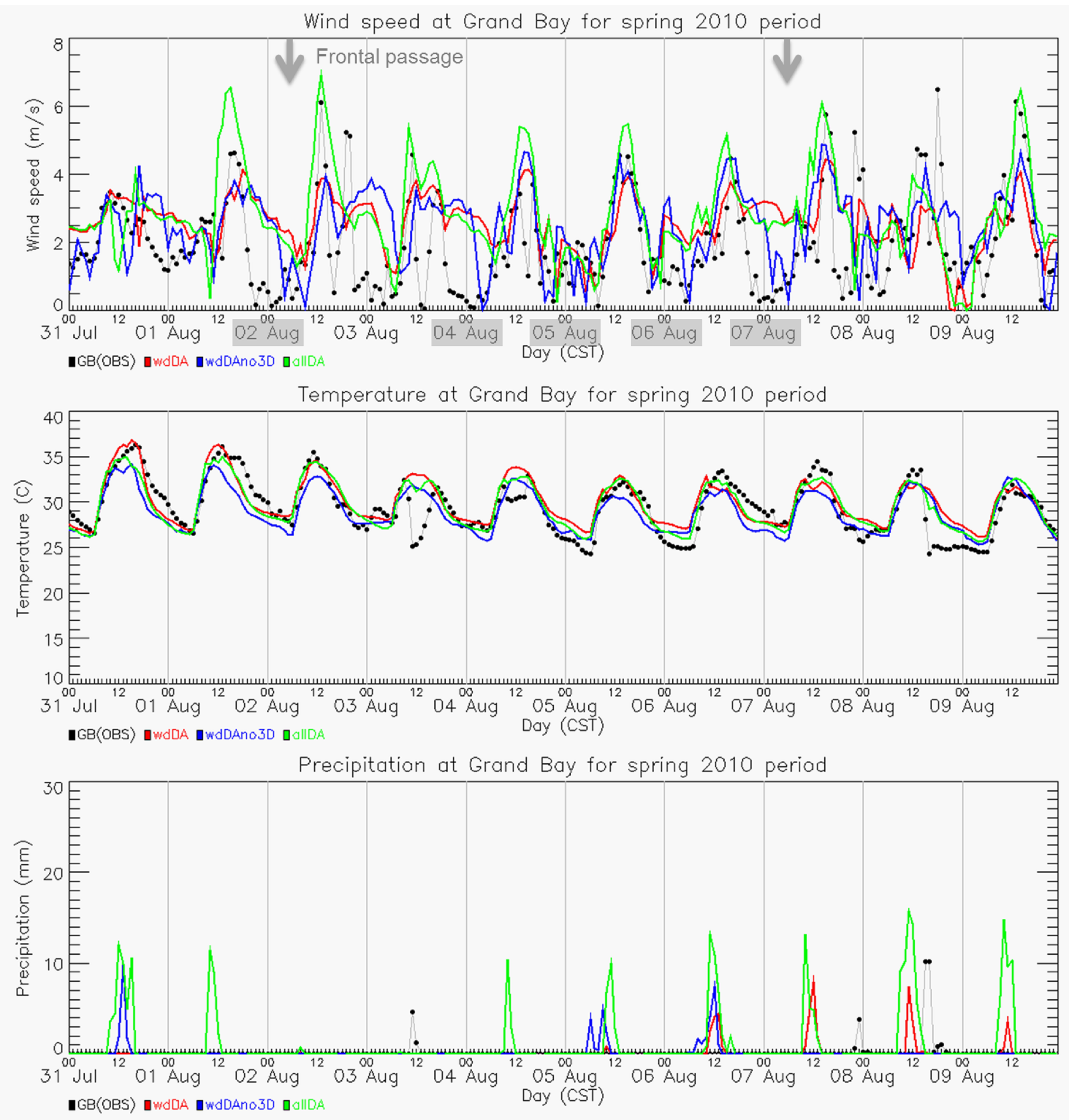
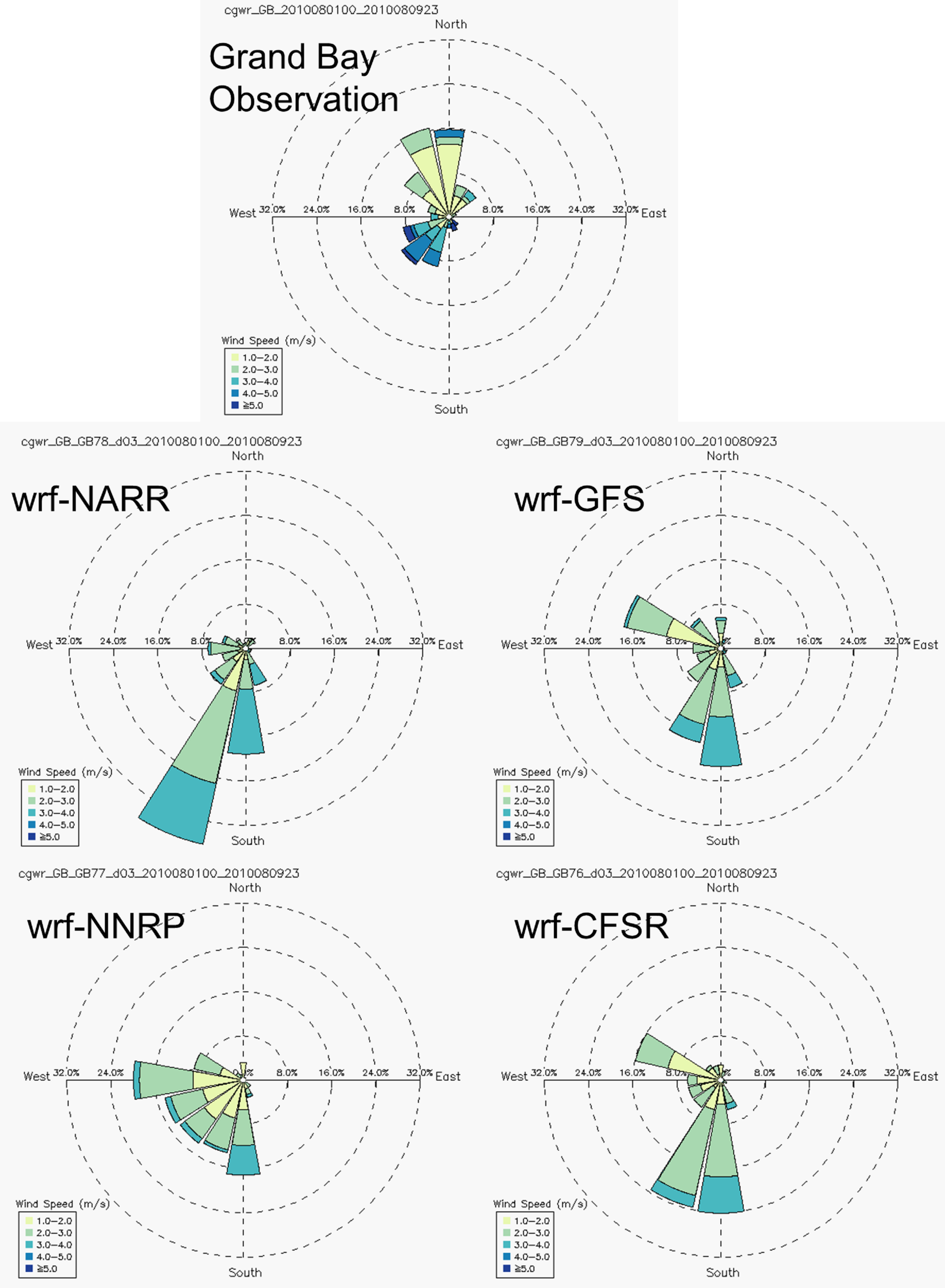
3.1. Meteorological Modeling for Summer 2010

3.1.1. Regional Evaluations

The statistical scores for each simulation were first computed by using MADIS surface data, which were also assimilated in the observational nudging, and then SCAN data, which were not used in the nudging. a comparison against the data from the Grand Bay NERR site is presented in the next section. Table 1 shows a comparison of the model performance by using the three different nudging configurations. It can be seen that the wdDA case (grid and observational nudging only for the u- and v-components of wind), outperformed the other two in predicting wind speed. The AllDA case, which used all nudging for wind, temperature and moisture, also had relatively good results, while the simulation without 3D grid nudging (wdDAno3D) had the worst statistical scores. Hence, the 3D grid nudging appears to improve wind predictions in this situation. Since allDA nudged both mass fields (temperature and moisture) and wind fields, perhaps not surprisingly, it exhibited better scores in temperature prediction. Table 2 compares MAE statistics by using the independent (i.e., not included in the objective analysis and nudging) SCAN observational data. It is evident that wdDA demonstrated the best skill at simulating wind speed and direction. The inclusion of mass fields in the nudging or removal of grid nudging degraded the accuracy of wind prediction in this application. For temperature and relative humidity, the MAE of the wdDAno3D simulation was lowest of all.
Table 1 also presents the model performance statistics (based on MADIS surface data) among cases using the four different reanalysis datasets for model initialization. For this comparison, the wdDA nudging scheme was used in each case. The best statistical scores for wind speed and direction were exhibited by the GFS case, while for surface temperature, the CFSR result was slightly better than the others. Note that the reanalysis data provide IC/LBC, as well as analysis fields for 3D grid nudging. The comparison with independent SCAN data in Table 2 shows that the NARR-based simulation was more accurate at predicting wind speed. For wind direction, the MAE for the CFSR-based simulation was slightly lower than the others, while for temperature and relative humidity, the GFS-based simulation exhibited the best performance.
Table 1. The statistical summary of the D03 domain for the summer 2010 intensive period computed by using the surface sites (METAR) from the Meteorological Assimilation Data Ingest System (MADIS). IC, initial conditions; LBC, lateral boundary conditions; SDE, standard deviation of the error; IOA, Index of Agreement; NARR, North American Regional Reanalysis; GFS, Global Forecast System; NNRP, NCEP-National Center for Atmospheric Research Reanalysis Product; CFSR, Climate Forecast System Reanalysis.
VariableIC/LBCNudgingRBiasRMSEMAESDEIOA
Wind speed
(m·s−1)
17,447 samples
WRF-NARRallDA0.684−0.1951.1270.8421.2850.819
WRF-NARRwdDAno3D0.6170.0221.2220.9381.5540.783
WRF-NARRwdDA0.716−0.2231.0490.7971.1760.831
Wind direction
(degree)
16,247 samples
WRF-GFSwdDA0.756−0.3391.0090.7571.0380.842
WRF-NNRPwdDA0.721−0.3401.0690.7991.1130.821
WRF-CFSRwdDA0.738−0.3331.0370.7771.0780.831
WRF-NARRallDA0.719−7.39670.22336.12375.5110.850
WRF-NARRwdDAno3D0.665−6.12276.29042.11484.1320.821
WRF-NARRwdDA0.731−5.56568.69235.01174.5290.857
WRF-GFSwdDA0.765−5.50465.57130.24669.8670.878
WRF-NNRPwdDA0.729−2.31968.98433.35475.6080.858
WRF-CFSRwdDA0.744−5.69367.78232.61272.7100.866
Temperature
(°C)
25,585 samples
WRF-NARRallDA0.940−0.0971.2250.8691.4440.966
WRF-NARRwdDAno3D0.830−0.2121.9921.5052.3660.901
WRF-NARRwdDA0.8500.0931.8711.3612.3680.915
WRF-GFSwdDA0.857−0.3561.8721.4102.1190.919
WRF-NNRPwdDA0.8530.1711.8641.3532.4010.853
WRF-CFSRwdDA0.864−0.2261.8041.3472.1120.923
Table 2. The MAE of the D03 domain for the summer 2010 intensive period computed by using the surface data from Soil Climate Analysis Network (SCAN).
ICBCNudgingWind Speed
(m·s−1)
3806 samples
Wind Direction
(degree)
3961 samples
Temperature
(°C)
4158 samples
Relative Humidity
(%)
4173 samples
WRF-NARRallDA1.18061.4252.2308.860
WRF-NARRwdDAno3D1.22260.4761.8587.663
WRF-NARRwdDA1.17159.6292.4828.912
WRF-GFSwdDA1.25160.6801.6518.334
WRF-NNRPwdDA1.36661.5661.7879.246
WRF-CFSRwdDA1.20758.7722.0218.806

3.1.2. Grand Bay Station Analysis

The meteorological observations at the Grand Bay site were not included in the data assimilation, similar to the SCAN data, meaning that they can be used as an independent dataset for the model evaluation. Table 3 shows a statistical summary (MAE) of model performance at this site based on a comparison with four soundings launched during the 2010 intensive. It can be seen that the influences of the reanalysis data through IC/LBC (and nudging) reached the finest domain (D03). Similar wind speed errors in the upper atmosphere were generated by the three nudging configurations. However, when grid nudging was turned off (wdDAno3D), larger MAEs were produced for wind direction, temperature and relative humidity. For this run, only observational nudging was operating, with the available data at the surface and aloft, including two soundings and one wind profiler in the study domain. The grid nudging used in the other configurations appears to have had a positive impact in the upper atmosphere on restraining the error growth. Among the four cases using different reanalysis data, the MAE scores of the GFS case were the lowest for wind prediction, except for relative humidity.
Table 3. The MAE of the D03 domain for the summer 2010 intensive period computed by using four soundings launched at Grand Bay.
ICBCNudgingWind Speed
(m·s−1)
392 samples
Wind Direction
(degree)
392 samples
Temperature
(°C)
392 samples
Relative Humidity
(%)
392 samples
WRF-NARRallDA1.64133.2740.63610.854
WRF-NARRwdDAno3D1.65641.5100.78014.003
WRF-NARRwdDA1.61332.3910.65211.254
WRF-GFSwdDA1.54831.7220.60715.003
WRF-NNRPwdDA2.05433.4690.7319.671
WRF-CFSRwdDA1.89830.4340.60313.425
WRF showed a good prediction for the 2-m temperature at the Grand Bay site during the daytime, but had a warm bias occasionally at nighttime (Figure 2, middle panel). The bottom panel of Figure 2 shows a time series of the modeled and observed precipitation at the Grand Bay site. There are several periods of modeled precipitation with no corresponding observations and several periods of observed precipitation without corresponding model predictions. Usually, a rapid drop in 2-m temperature associated with rain can be observed. The model missed the rainfall event on 3 August and did not predict the accurate timing of rain on 8 and 9 August. The Gulf area in the summer has abundant moisture available, and thunderstorms can easily be triggered. However, it is debatable if sub-grid-scale cloud parameterization should be used at 5–10-km resolutions, while at the same time, modeling using explicit cumulus schemes has not yet been successful [17,18]. Sensitivity tests on nudging configurations were carried out to determine if the model’s precipitation performance could be improved (Figure 2, lower panel). When temperature and moisture were nudged through grid and observational nudging (allDA), the model generated the most significant overestimates of precipitation. For daily accumulated rainfall over the entire D03 domain, the allDA nudging scheme produced 3–5-times more precipitation than the other two cases (figure not shown). Among all MADIS surface stations, we picked up sites where zero precipitations was recorded and corresponding model values for the comparison in Figure 3. It is noted that allDA has the largest overestimate of precipitation compared with the other two simulations using different nudging configurations. As some pollutants (e.g., GOM) are highly vulnerable to wet removal processes, extraneous precipitation would lead to artificially high wet deposition. Turning off the observational nudging for temperature and moisture (wdDA and wdDAno3D) reduced the precipitation overestimates somewhat. As can be seen from the top panel in Figure 2, these two nudging schemes did not produce large overestimates of wind speed at the Grand Bay site.
Figure 2. Time series of observed (dot-gray line) and modeled (various colors for different nudging configurations) (top) 10-m wind speed (m·s−1), (middle) 2-m temperature and (bottom) hourly precipitation (mm) at the Grand Bay site. Gray arrows indicate frontal passages, and mercury episodic days are highlighted with gray boxes.
Atmosphere 06 00209 g002
The surface wind comparisons in Figure 2 show that the model failed to predict the decrease in surface wind speed at night on certain days during the simulation period. This has been reported in other studies, such as those in Southeastern Texas [39,40] and the coastal cities of Spain [41]. On those days, a high pressure system was dominant over the study area and no precipitation was predicted, as shown in Figure 2. Possible causes of the overestimation of nocturnal wind speed could be the excessive vertical mixing simulated by the PBL scheme [39,40], the decoupling of the nocturnal boundary layer not properly simulated in the model [42] and/or the inaccuracy on predicting surface flux in the surface parameterization [43]. The wind rose plots (Figure 4) are the observed and model wind distribution at the Grand Bay site during the simulation period. All of the simulations generated too much south-southwesterly wind, while the measurement at Grand Bay was north-northwesterly dominant during the campaign period. For the wind speed, the observation had small values for northerly, but large values for southwesterly flows. The model re-produced strong southerly components of wind, but failed to generate a calm northerly. Examining the wind rose plots generated from the reanalysis data (not shown), we noticed that the reanalysis data that were input for WRF simulation lacked northerly components, while the wind measurement at Grand Bay station showed that the dominant wind was northerly. The NARR reanalysis had almost no northerly wind simulated, and the predominant wind directions were southerly to southwesterly. The model inherited features of the NARR reanalysis data, including the missing northerly components for the wind prediction.
Figure 3. Time series of hourly precipitation (inches) total accumulation over MADIS surface stations with zero precipitation for 2010 intensive (top) and 2011 intensive (bottom).
Atmosphere 06 00209 g003

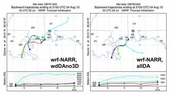
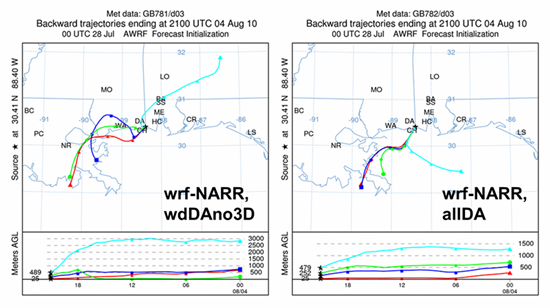
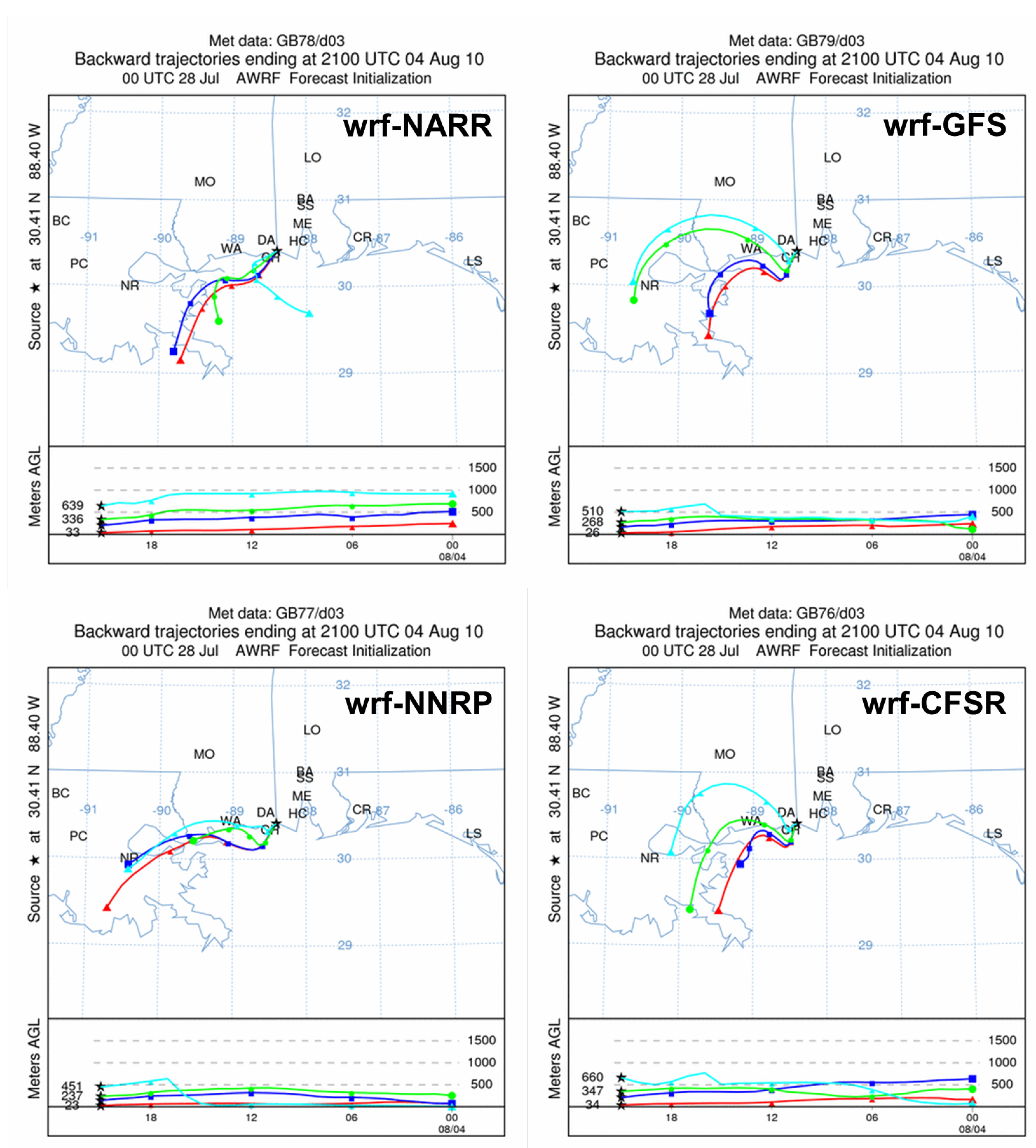
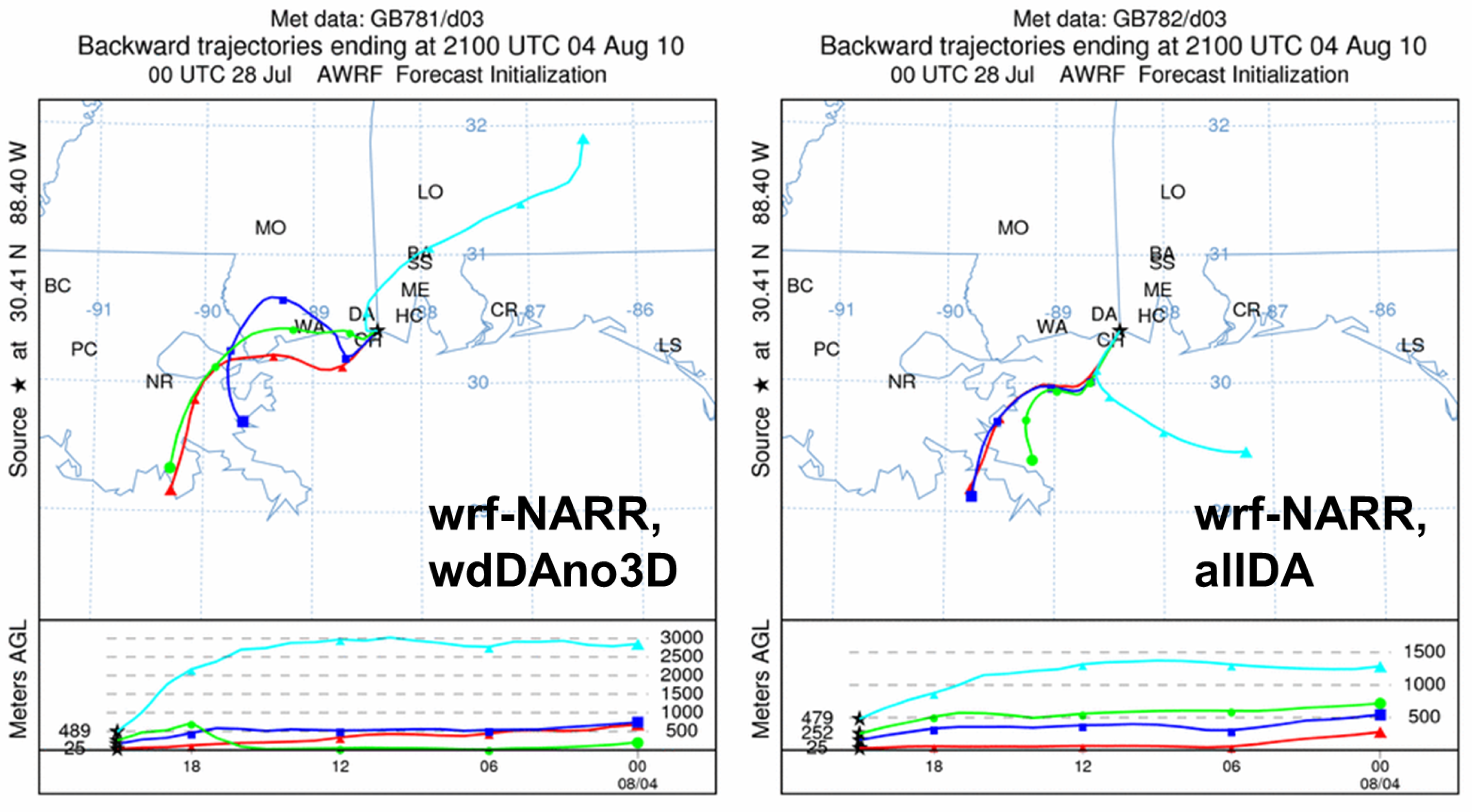
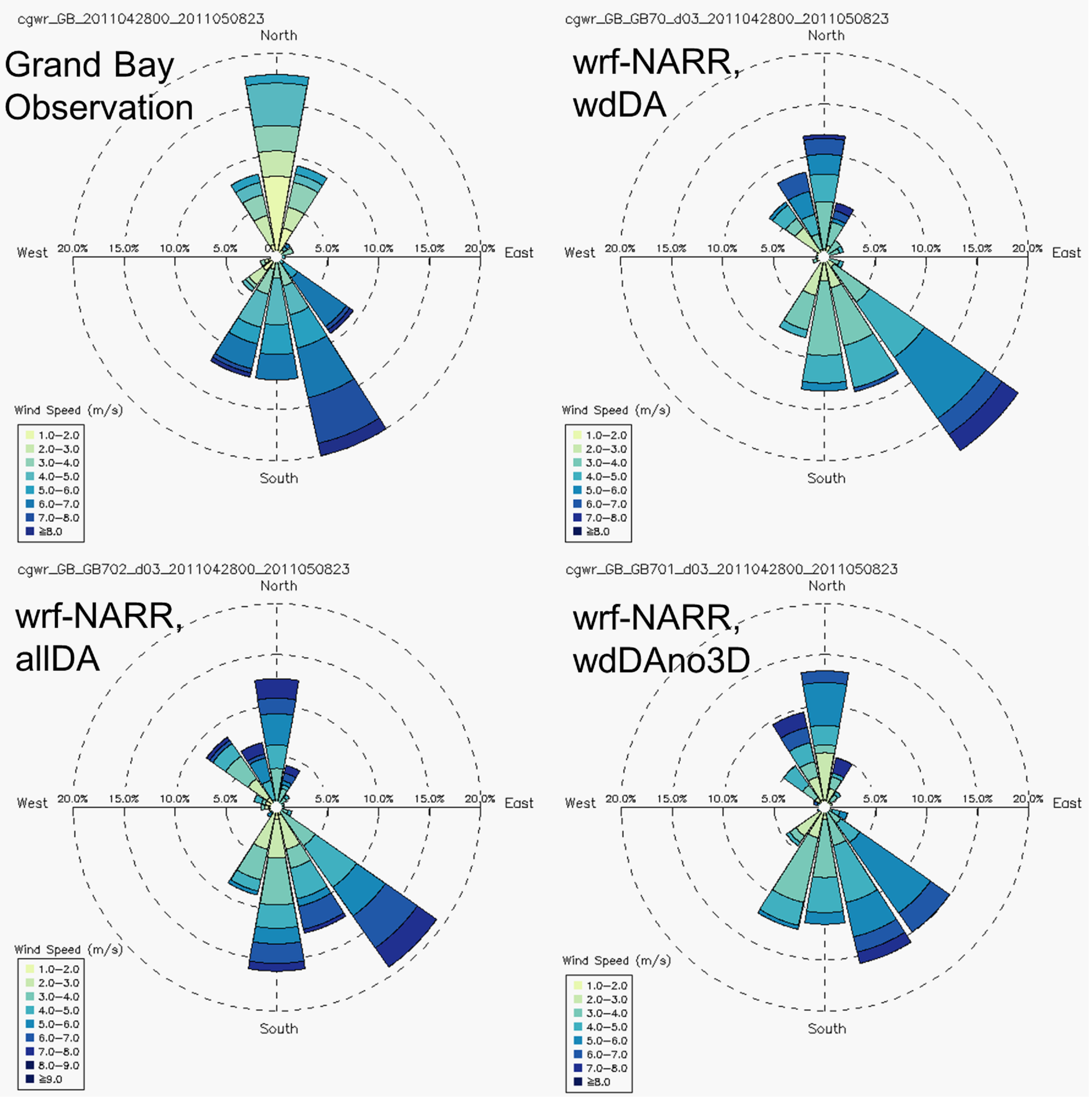
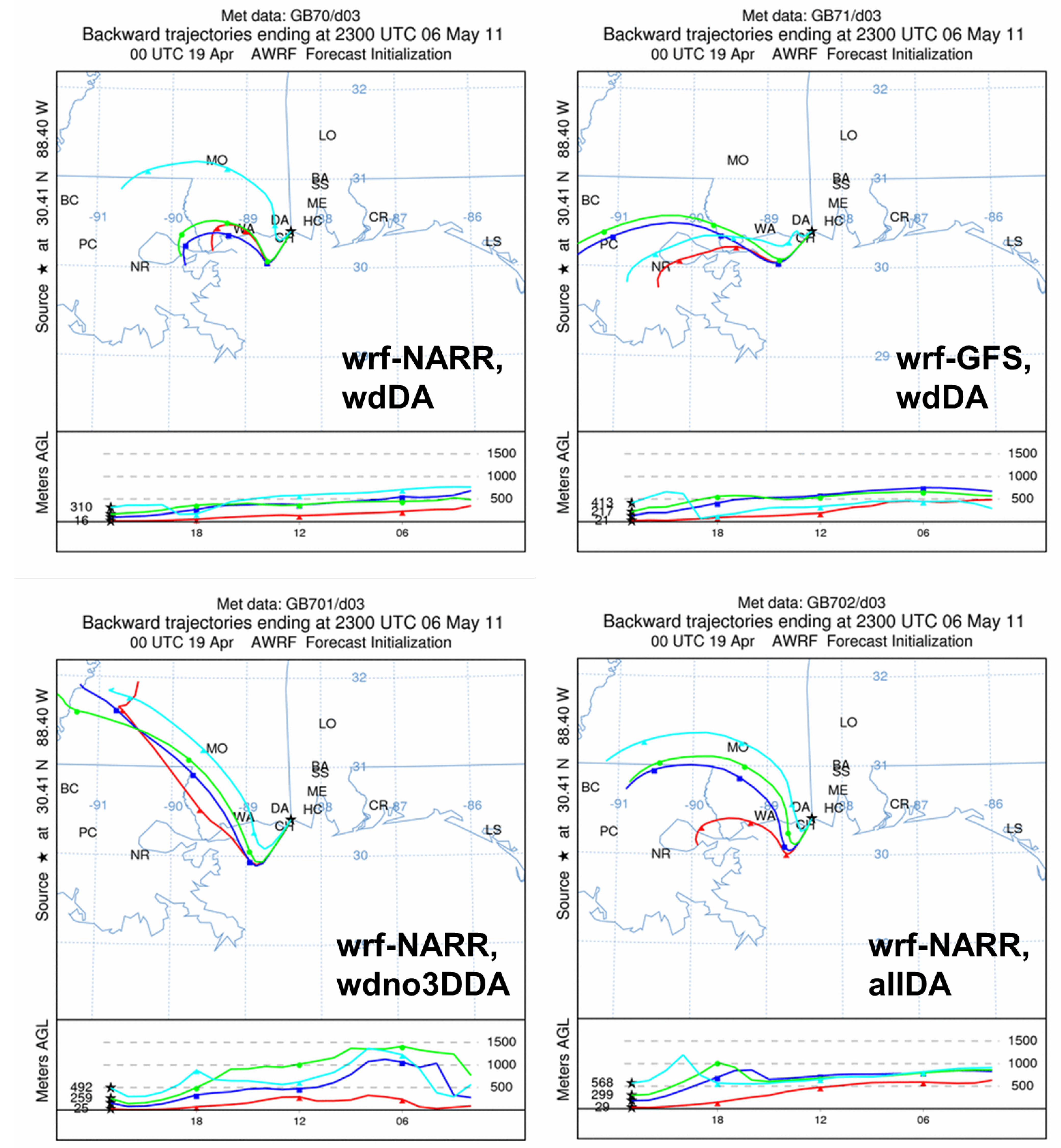
3.1.3. Backward Trajectory Analysis

On 4 August at 20:30 UTC, the GOM level reached 62 pg/m3 at the Grand Bay station, one of the highest measured GOM concentrations during the summer 2010 intensive period. During this peak, the measured surface wind direction at the site was southwesterly to westerly, while the wind speed was moderate, about 4 m·s−1. Backward trajectories (Figure 5) ending at 21:00 UTC on 4 August 2010, at Grand Bay were computed by HYSPLIT utilizing meteorological fields from WRF simulations initialized with different reanalysis data. Four starting altitudes, expressed as a fraction of the local model-estimated PBL height, were chosen: 0.05, 0.3, 0.5 and 0.95. The GFS-, NNRP- and CFSR-based simulations showed air parcels arriving at the site from the west, potentially bringing pollutants from sources in the west to Grand Bay. However, the NARR-based simulation indicated air masses coming from the Gulf, where the air would be expected to be relatively clean. The time series of the wind profile at Grand Bay (figure not shown) further showed that the NARR-based simulation predicted stronger and more southerly near surface winds compared with the GFS-based simulation. In this study, observations, including surface, profiler data and sounding, were used to adjust the reanalysis data (used for IC/BC and grid nudging) toward the observations through objective analysis. In addition, observations were directly used to nudge the predicted values during the simulation. With all of this “forcing” by observations and even with the three-nested domain configuration, the finest resolution domain still inherited differing features of reanalysis data, which resulted in different model-predicted regional wind patterns. The same backward trajectory configuration was applied for nudging cases (Figure 6). The wdDAno3D-based meteorology generated quite different backward trajectories when they were initiated at higher elevations (0.5 and 0.95 of the local model-estimated PBL height). Since the evaluation based on the Grand Bay sounding showed a larger error in wind direction prediction than the other cases, the northerly backward trajectories in the wdDAno3D case are likely to be unrealistic.

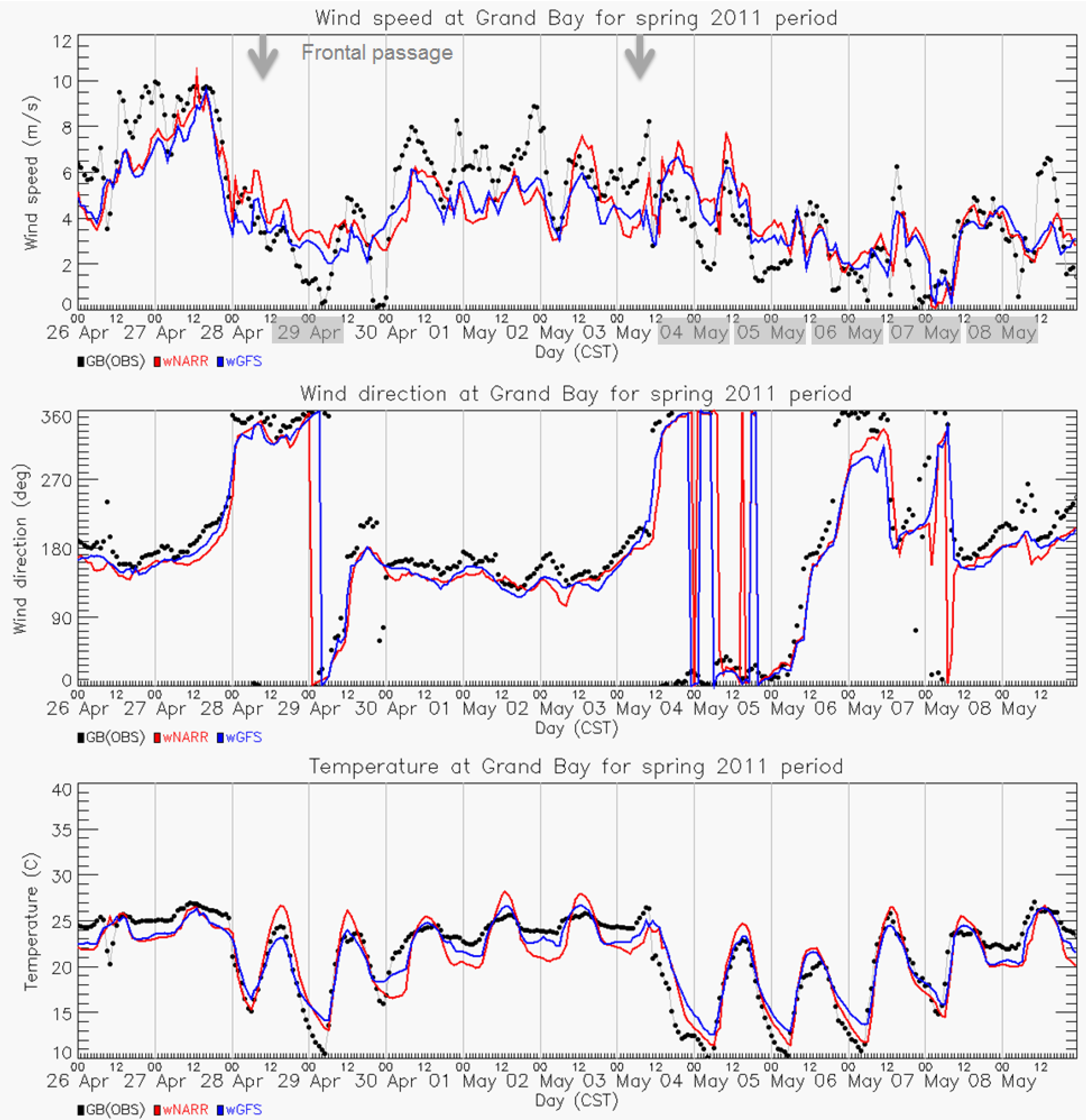
3.2. Meteorological Modeling for Spring 2011

3.2.1. Regional Evaluations

For the spring 2011 intensive period, all three nudging configurations conducted for the summer 2010 case were tested for the spring period, allowing us to further examine their performance in different seasons and meteorological conditions. To understand the variations in the reanalysis data, we focus efforts on evaluating the use of NARR and GFS datasets for modeling the spring episode. These are commonly used for the initialization of regional models in the community, and the benefit of using the other two datasets (NNRP and CFSR) for IC/LBC is not evident in the summer case.
Both simulations generated similar results for surface wind and temperature compared with the MADIS data. Consistent with the comparison with MADIS data for the summer 2010 intensive period, the nudging performed during the simulation successfully adjusted the predicted values toward the given observations. Table 4 shows the statistical summary of the model results evaluated against the independent SCAN data (i.e., data that were not used in the nudging). For mass fields (temperature and relative humidity), the NARR and GFS runs had similar statistical scores, while the NARR-based simulation performed slightly better for predicting wind speed and wind direction. Both wdDA and allDA had better scores for wind prediction, implying that the grid nudging for wind does help reduce the error for wind fields. The NARR case did generate wind fields as good as GFS in contrast to the summer case, for which NARR failed to re-produce southerly winds, as the GFS case did. The model over-predicted the amount of precipitation for a few days of the spring episode (Figure 3). AllDA had more days of rainfall overestimation than the other two cases, but overall, it was not as severe as the summer period.
Figure 4. Wind rose plots at Grand Bay station for four simulations using different reanalysis data for WRF initialization during the simulation period of the summer 2010 campaign.
Atmosphere 06 00209 g004
Figure 5. Backward trajectories ending at 21:00 UTC on 4 August 2010, at Grand Bay at multiple heights utilizing meteorological inputs from the NARR, GFS, NNRP and CFSR cases. Names in each plot indicate potential sources of mercury emissions.
Atmosphere 06 00209 g005

3.2.2. Grand Bay Station Analysis

As shown in the previous section with the summer intensive period, statistical summaries can only reveal the model’s performance in a general way. The examination of the time series of the meteorological variables at an individual site can yield further insights. Figure 6 shows the time series of 10-m wind speed, wind direction and the 2-m temperature at the Grand Bay site during the spring 2011 intensive period. Both the NARR- and GFS-based simulations predicted similar wind patterns, generally capturing the turning of the wind direction after the frontal passages on 28 April 28 and 3 May, as well as the dominant southerly flow between 30 April and 2 May. The NARR case did not appear to predict anomalous southerly winds at the Grand Bay site as it had for portions of the summer 2010 intensive period. The NARR-based simulation generally predicted a larger diurnal variation of 2-m temperature than the GFS case. This confirms the statistical scores that the surface temperature error was larger in the spring period than in the summer episode. Surface temperature may affect the prediction of the PBL height, but it is not a particularly influential parameter for dispersion modeling. Therefore, the inaccuracy of modeling the 2-m temperature is not expected to significantly affect the accuracy of the atmospheric mercury simulations using these data. The spring 2011 intensive period was less stormy than the earlier intensive; rain occurred before two frontal passages, but it did not last long. No precipitation was observed at Grand Bay on days with high atmospheric GOM concentrations (highlighted with gray boxes in Figure 7), and this lack of precipitation at the site was simulated well by the modeling.
Figure 6. Backward trajectories ending at 21:00 UTC on 4 August 2010, at Grand Bay at multiple heights utilizing meteorological inputs from the wdDAno3D and allDA cases. Names in each plot indicate potential sources of mercury emissions.
Atmosphere 06 00209 g006
The regional wind pattern is a critical factor in determining the transport of atmospheric mercury and other pollutants. Figure 8 shows the wind rose plots for surface wind over the entire innermost domain (D03) during the spring 2011 campaign. The surface wind distribution in the simulations with different initialization data was similar, in contrast with the modeling results for the summer 2010 intensive. The wind patterns from the reanalysis data represented closely matched the measurements at the Grand Bay station. Even though northerly components were somewhat under-represented, both NARR and GFS reanalysis reproduced two of the main wind patterns (northerly wind and southeasterly wind), as shown in the measurement. This finding suggests that the influence of the reanalysis data over the regional flow prediction is not always significant, but depends on the atmospheric conditions. Table 5 shows the model error (MAE) in the upper levels using data from the 10 soundings collected at Grand Bay during the spring 2011 intensive. All four variables had very similar MAE scores among the simulations with different model configurations. In the comparison of two intensive periods, the reanalysis data had a more obvious impact on WRF performance, even with regard to the innermost domain, in the summer campaign than the one conducted in spring.
Table 4. The statistical summary of the D03 domain for the spring 2011 intensive period computed by using SCAN data.
VariableIC/LBCNudgingRBiasRMSEMAESDEIOA
Wind speed
(m·s−1)
2768 samples
WRF-NARRallDA0.723−0.2682.0681.5652.4260.835
WRF-NARRwdDAno3D0.725−0.4072.0701.5712.3400.819
WRF-NARRwdDA0.738−0.4012.0301.5462.2960.832
WRF-GFSwdDA0.656−1.3392.6171.9662.3350.627
Wind direction
(degree)
2834 samples
WRF-NARRallDA0.5132.68875.44835.05784.3200.744
WRF-NARRwdDAno3D0.4001.24485.36541.83195.6090.683
WRF-NARRwdDA0.5021.47776.43135.58484.9300.737
WRF-GFSwdDA0.4718.02980.53039.09492.9580.718
Temperature
(°C)
2844 samples
WRF-NARRallDA0.9220.4662.2621.8163.1790.957
WRF-NARRwdDAno3D0.9040.2802.3091.8413.1230.948
WRF-NARRwdDA0.9100.4332.2961.8553.2120.951
WRF-GFSwdDA0.906−0.1372.2761.7592.7910.947
RH
(%)
2840 samples
WRF-NARRallDA0.8802.4759.6767.68313.8080.933
WRF-NARRwdDAno3D0.838−0.38912.2379.52015.2630.908
WRF-NARRwdDA0.847−1.35712.3999.64914.8550.909
WRF-GFSwdDA0.8374.23711.8799.41417.5930.901
Table 5. The MAE of the D03 domain for the spring 2011 intensive period computed by using the 10 soundings launched at Grand Bay.
ICBCNudgingWind Speed
(m·s−1)
978 samples
Wind Direction
(degree)
978 samples
Temperature
(°C)
978 samples
Relative Humidity
(%)
917 samples
WRF-NARRallDA1.69821.9380.9159.797
WRF-NARRwdDAno3D1.86921.8220.8958.825
WRF-NARRwdDA1.68322.0590.8388.575
WRF-GFSwdDA1.64920.1280.6268.432
Figure 7. Time series of observed (dot-gray line) and modeled (initialization with NARR and GFS data) (top) 10-m wind speed (m·s−1), (middle) 10-m wind direction and (bottom) 2-m temperature at the Grand Bay site. Gray arrows indicate frontal passages, and mercury episodic days are highlighted with gray boxes.
Atmosphere 06 00209 g007

3.2.3. Backward Trajectory Analysis

Backward trajectories were constructed by using the WRF meteorology results for air masses arriving at the Grand Bay site at 23:00 UTC on 6 May 2011 (Figure 9), when one of the highest GOM measurements (43.50 pg/m3) during the spring 2011 spring campaign occurred at 22:30 UTC of that day. Both simulations, using NARR and GFS for initialization, indicated that the air came from the west, northwest and/or north, passing in the vicinity of one or more emission sources that may have contributed to the peak. However, the trajectories using the GFS-based WRF results traveled longer distances than those generated by the NARR-based WRF results. The differences in wind speed and direction shown in the trajectory results would likely affect the dispersion modeling results from the relevant sources in the region. Although the wind roses were similar, the trajectories clearly showed persistent differences. Future work will examine the impacts of the use of different WRF model results on mercury dispersion in the vicinity of the Grand Bay site during the intensive periods.
Figure 8. Wind rose plots at Grand Bay for three simulations with different nudging configurations during the simulation period of the spring 2011 campaign.
Atmosphere 06 00209 g008
Figure 9. Backward trajectories ending at 23:00 UTC on 6 May 2011, at Grand Bay at multiple heights utilizing meteorological inputs generated by different configurations. The names in each plot indicate potential sources of mercury emissions.
Atmosphere 06 00209 g009

4. Conclusions

A site at the Grand Bay NERR station has been operated by the NOAA’s Air Resources Laboratory for the long-term monitoring of atmospheric mercury and other trace species since 2006. Two intensive measurement periods were conducted at the site in summer 2010 (from 28 July to 15 August) and spring 2011 (from 19 April to 9 May) to improve the understanding of the atmospheric fate and transport of mercury. To support mercury modeling in conjunction with the intensive, WRF-ARW was used to develop fine-resolution meteorological fields for the two campaign periods. Two sets of sensitivity tests were performed, to examine the influences on model performance and regional flow predictions: (1) the use of different reanalysis data for WRF initialization; and (2) the use of different nudging configurations. WRF simulations were evaluated with conventional observations and additional measurements, including surface and sounding data obtained at the Grand Bay station during the intensives. Backward trajectories using HYSPLIT were constructed for illustrative mercury peaks with different WRF meteorology to understand the influence of different meteorology inputs on the model-estimated source-receptor relationships at the site.
The nudging process in WRF sufficiently adjusted the model values toward the observations or analysis fields. The simulations by WRF with grid and observational nudging generated reasonable results and were in good agreement with the Grand Bay measurements. It was found that 3D grid nudging at the fine spatial grid (4-km resolution in this study), namely bringing the reanalysis data into the fine spatial grid, did not degrade model performance, but reduced errors in the wind predictions at the surface and aloft (the allDA and wdDA cases). The nudging of mass fields (temperature and moisture) had a significant impact on model-predicted precipitation, especially for the summer 2010 intensive period. In this case, mass-field nudging resulted in more extraneous precipitation at the Grand Bay site and 3–5-times more precipitation in the study domain than that generated in the simulations with the nudging of only wind components. These significant differences in modeled precipitation may have potentially large impacts on mercury fate and transport modeling, through the effects on wet deposition, and on the source-receptor relationships estimated from such modeling. The spring intensive period had much less precipitation than the summer case, and the WRF model simulated it relatively well.
The regional flow prediction can be influenced by the reanalysis data used to initialize and grid-nudge the WRF simulations. Larger differences were observed in the WRF results based on different reanalysis data in the summer campaign than in the spring campaign. For the 2010 summer period, the simulation using NARR data, commonly used for initializing the WRF model over North America domains, showed larger bias in comparison to the observations than the cases using other reanalysis data. Even with observational nudging, the fine-resolution domain still inherited differing features of the reanalysis data, which resulted in generating different regional wind patterns. The wind analysis at Grand Bay showed that the NARR case generated too much south-southwesterly wind compared with the other cases, and the observations actually showed north-northwesterly dominant winds during the campaign period. Similar wind patterns were generated among different sensitivity cases, but back-trajectory analyses were used to illustrate how even relatively small differences in regional wind fields can influence the modeled source-receptor relationships. In the example backward trajectory analysis of a summer 2010 mercury episode, the GFS-based simulation showed the air coming from the west, potentially bringing pollutants from emission sources to Grand Bay, while the NARR-based simulation showed air masses coming from the “clean” Gulf (i.e., with no large sources of mercury). The example trajectory analysis shown for the spring 2011 intensive also showed differences between the NARR- and GFS-based meteorological model results, but these were not as large as the difference shown in the summer 2010 episode. More differences between model results and measurements were observed between the various reanalysis datasets (used for model IC/BC/nudging) for the summer period than the spring campaign. According to the comparison of precipitation, the summer campaign period was stormier than the spring period. This may have led to higher uncertainties in the numerical model prediction during the summer period.
The 4-km grid spacing used here is generally considered to be at the borderline between the applicability of sub-grid cloud parametrizations (at larger grid spacing) and explicit approaches to generate convective updrafts (at smaller grid spacing). Future research will include simulations by using different microphysics schemes and cumulus parametrizations in the WRF model, as well as different grid sizes, to find the configuration(s) that give the best results. In addition, to improve the regional flow prediction, we will include the Grand Bay observations and SCAN dataset into the observational nudging, which may further reduce wind errors at those locations.

Acknowledgments

The authors thank Paul Kelly for his significant contribution to the data collection at the Grand Bay station.

Author Contributions

Fong Ngan wrote the majority of the manuscript and performed WRF simulations and model evaluations. Mark Cohen and Roland Draxler contributed valuable scientific insight and editing. Winston Luke and Xinrong Ren did the field campaigns at Grand Bay site, worked on data processing and quality control.

Conflicts of Interest

The authors declare no conflict of interest.

References

  1. Driscoll, C.T.; Manson, R.P.; Chan, H.M.; Jacob, D.J.; Pirron, N. Mercury as a global pollutant: Sources, pathways, and effects. Environ. Sci. Technol. 2013, 47, 4967–4983. [Google Scholar] [CrossRef] [PubMed]
  2. Cohen, M.; Artz, R.; Draxler, R.; Miller, P.; Poissant, L.; Niemi, D.; Ratte, D.; Deslauriers, M.; Duval, R.; Laurin, R.; et al. Modeling the atmospheric transport and deposition of mercury to the Great Lakes. Environ. Res. 2004, 47, 4967–4983. [Google Scholar]
  3. Cohen, M.; Artz, R.; Draxle, R. Report to Congress: Mercury Contamination in the Great Lakes; NOAA Air Resources Laboratory: Silver Spring, MD, USA, 2007. [Google Scholar]
  4. Evers, D.C.; Wiener, J.G.; Basu, N.; Bodaly, R.A.; Morrison, H.A.; Williams, K.A. Mercury in the Great Lakes region: Bioaccumulation, spatiotemporal patterns, ecological risks, and policy. Ecotoxicology 2011, 20, 1487–1499. [Google Scholar] [CrossRef] [PubMed]
  5. Harris, R.C.; Pollman, C.; Landing, W.; Evans, D.; Axelrad, D.; Hutchinson, D.; Morey, S.L.; Rumbold, D.; Dukhovskoy, D.; Adams, D.H.; et al. Mercury in the Gulf of Mexico: Sources to receptors. Environ. Res. 2012, 119, 42–52. [Google Scholar] [CrossRef] [PubMed]
  6. Butler, T.J.; Cohen, M.D.; Vermeylen, F.M.; Likens, G.E.; Schmeltz, D.; Artz, R.S. Regional precipitation mercury trends in the eastern USA, 1998–2005: Declines in the Northeast and Midwest, no trend in the Southeast. Atmos. Environ. 2008, 42, 1582–1592. [Google Scholar] [CrossRef]
  7. Engle, M.A.; Tate, M.T.; Krabbenhoft, D.P.; Kolker, A.; Olson, M.L.; Edgerton, E.S.; DeWild, J.F.; McPherson, A.K. Characterization and cycling of atmospheric mercury along the central U.S. Gulf Coast. Appl. Geochem. 2008, 23, 419–437. [Google Scholar] [CrossRef]
  8. Ren, X.; Luke, W.T.; Kelley, P.; Cohen, M.; Ngan, F.; Artz, R.; Walker, J.; Brooks, S.; Moore, C.; Swartzendruber, P.; et al. Mercury speciation at a coastal site in the northern Gulf of Mexico: Results from the Grand Bay Intensive Studies in summer 2010 and spring 2011. Atmosphere 2014, 5, 230–251. [Google Scholar] [CrossRef]
  9. Nair, U.S.; Wu, Y.; Holmes, C.D.; Schure, A.T.; Kallos, G.; Walters, J.T. Cloud-resolving simulations of mercury scavenging and deposition in thunderstorms. Atmos. Chem. Phys. 2013, 13, 10143–10210. [Google Scholar] [CrossRef]
  10. Draxler, R.R. An overview of the HYSPLIT_4 modeling system for trajectories, dispersion and deposition. Aust. Meteorol. Mag. 1988, 5, 230–251. [Google Scholar]
  11. Han, Y.J.; Holsen, T.M.; Hopke, P.K.; Yi, S.M. Comparison between back-trajectory based modeling and Lagrangian backward dispersion modeling for locating sources of reactive gaseous mercury. Environ. Sci. Technol. 2005, 39, 1715–1723. [Google Scholar] [CrossRef] [PubMed]
  12. Rolison, J.M.; Landing, W.M.; Luke, W.; Cohen, M.; Salters, V.J.M. Isotopic composition of species-specific atmospheric Hg in a coastal environment. Chem. Geol. 2013, 336, 37–49. [Google Scholar] [CrossRef]
  13. Gratz, L.E.; Keeler, G.J.; Marsik, F.J.; Barres, J.A.; Dvonch, J.T. Atmospheric transport of speciated mercury across southern Lake Michigan: Influence from emission sources in the Chicago/Gary urban area. Sci. Total Environ. 2013, 448, 84–95. [Google Scholar] [CrossRef] [PubMed]
  14. Lei, H.; Liang, X.Z.; Wuebbles, D.J.; Tao, Z. Model analyses of atmospheric mercury: Present air quality and effects of transpacific transport on the United States. Atmos. Chem. Phys. 2013, 13, 10807–10825. [Google Scholar] [CrossRef]
  15. Skamarock, W.C.; Klemp, J.B.; Dudhia, J.; Gill, D.O.; Barker, D.M.; Duda, M.G.; Huang, X.Y.; Wang, W.; Powers, J.G. A description of the advanced research WRF Version 3. In NCAR Technical Note; NCAR: Boulder, CO, USA, 2008; TN-475+STR. [Google Scholar]
  16. W., W.; Lynch, A.H.; Rivers, A. Estimating the uncertainty in a regional climate model related to initial and lateral boundary conditions. J. Appl. Climatol. 2005, 18, 917–933. [Google Scholar] [CrossRef]
  17. Ngan, F.; Byun, D.W.; Kim, H.C.; Lee, D.G.; Rappenglueck, B.; Pour-Biazar, A. Performance assessment of retrospective meteorological inputs for use in air quality modeling during TexAQS 2006. Atmos. Environ. 2012, 54, 86–96. [Google Scholar] [CrossRef]
  18. Deng, A.; Stauffer, D.; Gaudet, B.; Dudhia, J.; Hacker, J.; Bruyere, C.; Wu, W.; Vandenberghe, F.; Liu, Y.; Bourgeois, A. Update on WRF-ARW end-to-end multi-scale FDDA system. In Proceedings of the 10th WRF Users’ Workshop, Boulder, CO, USA, 23–26 June 2009; NCAR: Boulder, CO, USA, 2009. [Google Scholar]
  19. Otte, T. The impact of nudging in the meteorological model for retrospective air quality simulations. Part I: Evaluation against national observation networks. J. Appl. Meteor. Climatol. 2008, 47, 1853–1867. [Google Scholar]
  20. Lo, J.C.F.; Yang, Z.L.; Sr, R.A.P. Assessment of three dynamical climate downscaling methods using the Weather Research and Forecasting (WRF) model. J. Geophys. Res. 2008. [Google Scholar] [CrossRef]
  21. Godowitch, J.M.; Gilliam, R.C.; Rao, S.T. Diagnostic evaluation of ozone production and horizontal transport in a regional photochemical air quality modeling system. Atmos. Environ. 2011, 45, 3977–3987. [Google Scholar] [CrossRef]
  22. Rogers, R.; Deng, A.; Stauffer, D.R.; Gaudet, B.J.; Jia, Y.; Soong, S.; Tanrikulu, S. Application of the weatherresearch and forecasting model for air quality modeling in the San Francisco bay area. J. Appl. Meteor. Climatol. 2013, 52, 1953–1973. [Google Scholar] [CrossRef]
  23. Hegarty, J.; Coauthors. Evaluation of Lagrangian particle dispersion models with measurements from controlled tracer releases. J. Appl. Meteor. Climatol. 2013, 52, 2623–2637. [Google Scholar] [CrossRef]
  24. Gilliam, R.C.; Godowitch, J.M.; Rao, S.T. Improving the horizontal transport in the lower troposphere with four dimensional data assimilation. Atmos. Environ. 2012, 53, 186–201. [Google Scholar] [CrossRef]
  25. Mlawer, E.; Taubman, S.; Brown, P.D.; Iacono, M.; Clough, S. Radiative transfer for inhomogeneous atmosphere: RTTM, a validated correlated-k model for the longwave. J. Geophys. Res. 1997, 102, 16663–16682. [Google Scholar] [CrossRef]
  26. Dudhia, J. Numerical study of convection observed during the winter monsoon experiment using a mesoscale two-dimensional model. J. Atmos. Sci. 1989, 46, 3077–3107. [Google Scholar] [CrossRef]
  27. Xiu, A.; Pleim, J.E. Development of a land surface model. Part I: Application in a mesoscale meteorological model. J. Appl. Meteor. 2001, 40, 192–209. [Google Scholar] [CrossRef]
  28. Pleim, J.E.; Xiu, A. Development of a land surface model. Part II: Data assimilation. J. Appl. Meteor. 2003, 42, 1811–1822. [Google Scholar] [CrossRef]
  29. Pliem, J.E. A combined local and nonlocal closure model for the atmospheric boundary layer. Part I: Model description and testing. J. Appl. Meteor. Climatol. 2007, 46, 1383–1395. [Google Scholar] [CrossRef]
  30. Grell, A.G.; Devenyi, D. A generalized approach to parameterizing convection combining ensemble and data assimilation techniques. J. Geophys. Res. Lett. 2002. [Google Scholar] [CrossRef]
  31. Mesinger, F.; DiMego, G.; Kalnay, E.; Mitchell, K.; Shafran, P.C.; Ebisuzaki, W.; Jovic, D.; Woollen, J.; Rogers, E.; Berbery, E.H.; et al. North American regional reanalysis. Bull. Am. Meteor. Soc. 2006, 87, 343–340. [Google Scholar] [CrossRef]
  32. Kanamitsu, M. Description of the NMC global data assimilation and forecast system. Weather Forecast. 1989, 4, 334–342. [Google Scholar]
  33. Kalnay, E.; Kanamitsu, M.; Kistler, R.; Collins, W.; Deaven, D.; Gandin, L.; Iredell, M.; Saha, S.; White, G.; Woollen, J.; et al. The NCEP/NCAR 40-year reanalysis project. Bull. Am. Meteor. Soc. 1996, 77, 437–471. [Google Scholar] [CrossRef]
  34. Saha, S.; Moorthi, S.; Pan, H.-L.; Wu, X.; Wang, J.; Nadiga, S.; Tripp, P.; Kistler, R.; Woollen, J.; Behringer, D.; et al. The NCEP climate forecast system reanalysis. Bull. Am. Meteor. Soc. 2010, 91, 1015–1057. [Google Scholar] [CrossRef]
  35. Chai, T.; Draxler, R.R. Root mean square error (RMSE) or mean absolute error (MAE)?—Arguments against avoiding RMASE in the literature. Geosci. Model Dev. 2014, 7, 1247–1250. [Google Scholar]
  36. Gilliam, R.; Hogrefe, C.; Rao, S. New methods for evaluating meteorological models used in air quality applications. Atmos. Environ. 2006, 40, 5073–5086. [Google Scholar] [CrossRef]
  37. Yu, S.; Rohit, M.; Pleim, J.; Pouliot, G.; Wong, D.; Eder, B.; Schere, K.; Gilliam, R.; Rao, S. Comparative evaluation of the impact of WRF-NMM and WRF-ARW meteorology on CMAQ simulations for O3 and related species during the 2006 TexAQS/GoMACCS campaign. Atmos. Pollut. Res. 2012, 3, 149–162. [Google Scholar]
  38. Wilks, D. Statistical Methods in the Atmospheric Sciences; Elsevier: Burlington, MA, USA, 2006; p. 549. [Google Scholar]
  39. Lee, S.-H.; Kim, S.-W.; Angevine, W.M.; Bianco, L.; McKeen, S.A.; Senff, C.J.; Trainer, M.; Tucker, S.C.; Zamora, R.J. Evaluation of urban surface pa- rameterizations in the WRF model using measurements during the Texas Air Quality Study 2006 field campaign. Atmos. Chem. Phys. 2011, 11, 2127–2143. [Google Scholar] [CrossRef]
  40. Ngan, F.; Kim, H.; Lee, P.; Al-Wali, K.; Dornblaser, B. A study of nocturnal surface wind speed overprediction by the WRF-ARW model in southeastern Texas. J. Appl. Meteor. Climatol. 2013, 52, 2638–2653. [Google Scholar] [CrossRef]
  41. Chen, B.; Stein, A.F.; Castell, N.; de laRosa, J.D.; de laCampa, A.; Gonzalez-Castanedo, Y.; Draxler, R.R. Modeling and surface observations of arsenic dispersion from a large Cu-smelter in southwestern Europe. Atmos. Environ. 2012, 49, 114–122. [Google Scholar] [CrossRef]
  42. Zhang, D.; Zheng, W. Diurnal cycles of surface winds and temperatures as simulated by five boundary layer parameterizations. J. Appl. Meteor. 2004, 1, 157–169. [Google Scholar] [CrossRef]
  43. Tong, D.; Lee, P.; Ngan, F.; Pan, L. Investigation of Surface Layer Parameterization of the WRF Model and Its Impact on the Observed Nocturnal Wind Speed Bias: Period of Investigation Focuses on the Second Texas Air Quality Study (TexAQS II) in 2006. Available online: http://aqrp.ceer.utexas.edu/index.cfm (accessed on 16 February 2015).

