1. Introduction
Houston, the fourth largest city in the United States, is located on the northern coastline of the Gulf of Mexico [
1]. It routinely experienced some of the highest ozone (O
3) mixing ratios in the United States over the past several decades [
2]. Due to this it has been classified by the U.S. Environmental Protection Agency as a “severe” 8-h O
3 nonattainment area in 1997 and a “marginal” 8-h O
3 nonattainment area in 2008 [
3]. Houston experienced significant variability in both the peak O
3 mixing ratios and the number of high O
3 days [
4]. Houston exceeds the 75 ppbv 8-h and 124 ppbv 1-h National Ambient Air Quality Standard (NAAQS) for ground-level O
3 mixing ratios dozens of days a year over last two decades [
4].
The Texas Commission on Environmental Quality (TCEQ) treats the O
3 mixing ratio at a given location as the sum of the background mixing ratio and the contribution from local O
3 production [
5]. Background O
3 levels in eastern Texas are typically higher during late summer and early fall as northerly and easterly flows associated with synoptic scale transport of O
3-rich continental air to the region [
6]. This increased regional background contributes to the frequency and severity of high-O
3 episodes in Houston [
7].
Air pollution in the Houston area is a product of strong emissions coupled with specialized meteorological conditions [
8]. Automobiles and industrial sources along the Houston Ship Channel (HSC) area and in outlying areas of the city emit large amounts of highly reactive volatile organic compounds (HRVOCs) and nitrogen oxides (NO + NO
2 = NO
x) [
8,
9], which provides the ingredients necessary for ground-level O
3 production in the presence of heat and sunlight [
10].
More than 400 chemical manufacturing facilities and two of the four largest refineries in the U.S. reside in the Houston Ship-Channel area [
11]. As a world-class city, the population of Houston increased 29% in the past two decades [
12]. This has led to increased vehicular traffic and associated NO
x emissions [
13]. Inevitably, this caused environmental problems, especially with regard to air pollution. Air pollution effects the health of human beings [
14], impacts radiative transfer in the atmosphere [
15], and how much solar ultraviolet radiation reaches the ground [
16,
17]. Houston has moved from #7 to #6 in the rankings of the worst O
3 in the U.S., which is based on the number of days with elevated pollution levels [
18]. As the air pollution conditions grew worse, researchers and policy makers started to pay attention to this topic. In 2000, the city of Houston started an emission reduction plan that focused on reduction of NO
x emissions from industry and motor vehicles [
19]. The National Oceanographic and Atmospheric Administration (NOAA) conducted two airborne studies in the Houston area; Texas Air Quality Study I 2000 [
20] and the Texas Air Quality Study II—the Gulf of Mexico Atmospheric Composition and Climate Study 2006 [
21]. These studies involved both measurements and modeling to unravel the complexity of air pollution in Houston and especially to understand what was driving the unusually high O
3 production in the area.
Meteorology also plays a critical role in O
3 formation, which either dilutes pollutant emissions or allows them to accumulate, and it can also affect other key processes, such as chemical reaction rates [
22,
23]. Previous studies have shown that levels of O
3 precursors are substantially elevated during post-frontal environments or in the presence of anti-cyclonic conditions where weak winds, clear skies, and subsidence dominates [
5,
23,
24].
In this paper, we characterized various meteorological variables including temperature, wind speed, wind direction, and pressure for both high and low O
3 events over the past 23 years (from January 1990 to December 2013). We obtained in-depth understandings about the relationship between the climate/meteorology factors and O
3 mixing ratios in the Houston area. Because Houston is located (latitude 30°) near the northern coast of the Gulf of Mexico, it is known that ground-level O
3 mixing ratios could be affected significantly by the land-sea breeze [
25].
We choose four sites along the South-North direction in the Houston area. We mainly emphasized trends of ground-level O3 mixing ratios, background O3 mixing ratios, wind speed, wind direction, temperature and pressure. A critical question to answer is, which is the key meteorology factor that influences concentration of ground-level O3 on a large time scale in the Houston area?
2. Results and Discussion
2.1. Background O3
Background O
3 is the mixing ratio of O
3 in the absence of direct influence by local anthropogenic emissions in an area [
7]. Currently, the 8-h O
3 standard is 75 ppb (the 84 ppb standard was changed in 2008) [
26], the ongoing reduction of 1-h and 8-h standards makes the level of background O
3 more important. Background O
3 levels vary with time of day, over months, and across large time spans of a decade or more [
7]. Changes in natural and anthropogenic sources during long-range atmospheric transport will ultimately influence local O
3 levels. In the Houston area, background O
3 mixing ratio trends are flat or decreasing, and vary strongly with transport patterns [
7]. For example, the flow of air from over the Gulf of Mexico may play an important role in the Houston background O
3 levels. Carbon monoxide is an excellent anthropogenic tracer because it mostly comes from mobile combustion [
27]. Air masses with CO mixing ratios below the 25th percentile value are commonly considered background air [
27]. In this study, we used the 20th percentile ofconcurrently measured carbon monoxide (CO) and O
3 to ascertain background O
3 [
28]. These measurements were performed atop Moody Tower on the University of Houston campus over the time period of January 2008 to January 2014.
Figure 1 shows a time series of the background O
3 mixing ratios in urban Houston.
Figure 1.
Monthly averaged background O3 mixing ratios measured atop Moody Tower on the University of Houston campus.
Figure 1.
Monthly averaged background O3 mixing ratios measured atop Moody Tower on the University of Houston campus.
Background O3 ranged between 15 ppbv and 45 ppbv, with an average of 30 ppbv and the highest values occurring in spring and lowest in June or July. During the summer there is strong southerly flow off the Gulf of Mexico bringing “cleaner” air inland. The overall trend-line shows that background O3 is fairly constant with a slight decrease of ~1 ppbv over the past seven years.
2.2. Exceedance Days of 1-h/8-h Averaged O3 Mixing Ratio
We analyzed data from the four research sites around the urban Houston. According to the revised National Ambient Air Quality Standards (NAAQS) by the Environmental Protection Agency (EPA) in 2011, for ground-level O3 if there is at least one 1-h averaged surface O3 mixing ratio exceeding 124 ppbv or an 8-h average exceeding 75 ppbv, the day is regarded as an exceedance day.
In
Figure 2 we illustrate the number of exceedance days of 1-h and 8-h averaged ground-level O
3 for each year during the research period 1990 to 2013 for our four sites. Note that the available O
3 mixing ratio data for the Galveston site only goes back to 1997 instead of 1990. The four sites’ number of exceedance days of 1-h averaged O
3 and 8-h averaged O
3 remained with wide year-to-year variations. We find that the most northern sites (
i.e., Aldine and Northwest Harris) have higher occurrences of exceedance days than the sites to the south (
i.e., Clinton and Galveston). Surface O
3 is a secondary product that is formed during transport, and under southerly winds the highest O
3 would be expected in the northern part of the study area.
Figure 2.
Annually exceedance days of 1-h averaged (a) and 8-h averaged (b) O3 mixing ratios during 1990–2014 for four sites.
Figure 2.
Annually exceedance days of 1-h averaged (a) and 8-h averaged (b) O3 mixing ratios during 1990–2014 for four sites.
The dashed lines on
Figure 2 are the linear trend lines of the exceedance days over the 23 year period. The slopes of the 1-h and (8-h) trend lines are −0.69 year
−1 (−1.5 year
−1) (Aldine), −0.50 year
−1 (−1.0 h
−1) (Northwest Harris), −0.60 year
−1 (−0.90 year
−1) (Clinton), and −0.39 year
−1 (−1.8 year
−1) (Galveston).From
Figure 2, we noticed that around the year of 2000, the number of exceedance days at all sites dropped dramatically. After 2000, the number of exceedance days remained steady in the low single digits. We attribute a reduction in emissions for part of this transition to lower O
3 mixing ratios in Houston. We divided the time period shown in
Figure 2 into two stages: the first stage was 1990–2000 and the second stage was 2001–2013. We calculated the average number of exceedance days for each site during the two stages. As
Table 1 shows, the average number of exceedance days at Aldine decreased from 12 to 2 (1-h) and from 35 to 11 (8-h); at Clinton they decreased from 10 to 2 (1-h) and 20 to 8 (8-h); NW Harris they decreased from 9 to 1 (1-h) and 28 to 13 (8-h); at the Galveston site they decreased from 6 to 1 (1-h) and from 29 to 8 (8-h). The average number of exceedance days during stage II was reduced to about one-fifth of the stage I for 1-h averaged O
3, and reduced to half of its original value for the 8-h averaged O
3.
Table 1.
Average Number of Exceedance Days per Site 1-h (8-h).
Table 1.
Average Number of Exceedance Days per Site 1-h (8-h).
| Site | 1990–2000 | 2001–2013 |
|---|
| Aldine | 12 (35) | 2 (11) |
| Clinton | 10 (20) | 2 (8) |
| NW Harris | 9 (28) | 1 (13) |
| Galveston | 6 (29) | 1 (8) |
2.3. Southerly Flow and Ground-Level O3
We analyzed the long-term relationship between ground-level O
3 mixing ratio and meteorological factors, including temperature, pressure, and wind speed. However, we did not find any significant relationships. The analyzed results can be found in the
Supplementary Material (Figures S1 and S2).
According to the research of Banta
et al. [
25], summertime meteorological conditions in Houston involve interactions between sea-breeze circulation patterns. The sea-breeze cycle at 30° N latitude is at maximum amplitude [
25]. It plays an especially strong role for atmospheric advection in the Houston area. There are two forms of the sea breeze in Houston: (1) the superposition of large-scale flow with inertia-gravity wind oscillation [
25]; and (2) under suitable conditions of wind and temperature, the sea breeze can assume a frontal structure. Both of these can produce winds inland away from the shore. Banta
et al. [
25] and Rappengluck
et al. [
24] showed that under specialized conditions (e.g
., timing, location, and the height to which pollutants mix), the pollutants that have been carried offshore by the land breeze can be brought back over land by the sea breeze. Southerly winds typically bring in “cleaner” marine with lower precursors (e.g., NO
x, CO, and hydrocarbons) and lower background levels of O
3 [
24].
Especially in the summer and fall seasons, southerly flow can influence local air quality conditions. A common pattern that was found is, in the early morning, northerly winds push polluted air masses aloft in the Galveston area, which is located next to the Gulf of Mexico. Around noontime to the early afternoon, because of the increased solar radiation and the higher heat capacity of water, land temperatures increase faster than water temperatures, and the sea breeze (southerly flow) with relative “cleaner” air, which originated over the Gulf of Mexico begins to appear over the city [
25]. According to our data analysis, in the late afternoon, especially during 2:00 p.m.~5:00 p.m. in summer and fall seasons, the air temperature and the frequency of southerly flow reach the peak. However, when night falls, air temperature decreases dramatically because of the lack of solar radiation. Along with it, there is a disappearance of the sea breeze and northerly winds take over again (
i.e., the land breeze). Local emissions trapped under a shallow nocturnal planetary boundary layer (PBL) accelerate the accumulation of pollutants in downtown Houston and the Houston-Ship-Channel areas.
Figure 3.
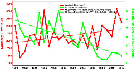
1-h and 8-h exceedance days as a function of annual southerly flow hours per year at the Aldine site.
Figure 3.
1-h and 8-h exceedance days as a function of annual southerly flow hours per year at the Aldine site.
To further investigate the variations of southerly wind, we defined the range of wind directions for southerly flow as 160°–200° and only examined the wind data during March-October, the southerly flow season [
25]. We used meteorological data from the NOAA Climate Data Center, which provided one-hour averaged wind speed and wind direction information. In order to get an in-depth understanding, we contrasted the two factors. The relationship between annually number of exceedance days and hours of southerly flow per year is depicted in
Figure 3 (Aldine) and
Figure 4 (Clinton). The anti-correlation between these two parameters is striking, and shows that the length of time per year Houston is under the influence of southerly flow has more than doubled from 1990 to 2013. The correlation coefficient between annually southerly flow hours and annually number of exceedance days of 1-h averaged (8-h averaged) in Aldine site are −0.63 (−0.72), for Clinton site are −0.56 (−0.51). All of them pass the significant test (
p < 0.05). The slope of the linear regression line for 1-h exceedance days at Aldine is −0.71 exceedances year
−1 and −0.90 exceedances year
−1 at Clinton. Conversely, the slope for Aldine is +56.6 southerly h year
−1 and +16.8 southerly h year
−1 for Clinton. Similar relationships for the two other sites can be found in the
Supplementary Material (Figures S3 and S4). The Clinton site is near downtown Houston and the ship channel area where many refineries and petrochemical industrial plants are located. In addition, the slope of southerly flow hours is more than three time greater at Aldine than at Clinton. These nearby sources and reduced dilution likely supplied more O
3 precursor compounds to this site and slowed the trend in decreased O
3.
Figure 4.
1-h and 8-h exceedance days as a function of annual southerly flow hours per year at the Clinton site.
Figure 4.
1-h and 8-h exceedance days as a function of annual southerly flow hours per year at the Clinton site.
We propose that the increased flow of “cleaner” air is diluting the dirty Houston air, lowering the mixing ratios of NO
x, O
3, and precursor hydrocarbons. It also would advect the polluted air away from Houston. Both of these processes would lead to a lower potential to produce O
3 in the Houston area. The significantly increased southerly flow together with lower emissions is leading to a “cleaner” O
3 environment. The general correspondence between increased exceedance days and decreased southerly flow hours give credence to our hypothesis. For example, the 8-h peak value was 55 with the corresponding low in southerly flow hours of 500 (
Figure 3).
2.4. Contrasting Southerly Flow Frequencies
We have documented increased southerly flow hours from 1990 to 2013, and now will examine this in terms of southerly flow days and averaged daily southerly flow hours. Around the year 2000, there was a decrease in the number of exceedance days; they dropped dramatically and decreased by a factor of three on average. After 2000 the number of exceedance days was decreased to single digits, meanwhile southerly flow hours increased steadily by a factor of two. Based on the changes, we divided the time series into two stages: 1990–2000 and 2001–2013. In each stage we choose two sample years when most of the data were close to the trend-line and with good representatives. We choose 1995 and 1996 for stage I, and 2010 and 2011 for stage II. The data of the sample years were averaged to better compare the southerly flow between the two stages. We compared Aldine site located north of the urban Houston area and the Galveston site close to the Gulf of Mexico (
Figure 5). Southerly flow mainly occurs in summer and fall season when the sea surface temperature has the largest gradients with land temperature. We examined the data of March–October to cover the period of southerly flow conditions. It is apparent at both sites that annually southerly flow hours have increased dramatically, by as much as a factor of 2–3. The inland sites experienced greater increases in southerly flow hours than the Galveston site. Both of the two sites had the strongest southerly flow in May, June and July. In 2010 and 2011 the Aldine site had the strongest southerly flow in April and June, slightly earlier in the year.
In Galveston 65% of the southerly flow occurred in summertime, specifically, in June, July and August. Annually southerly flow hours in June (from 200 to 350), August (from 120 to 380) and October (from 60 to 200) increased the most, increasing by a factor of 2.5 on the average. In the summer season southerly flow dominates in Galveston.
Figure 5.
Total southerly flow average hours in 1995–1996 (black) and 2010–2011 (red) at Aldine (a) and Galveston (b).
Figure 5.
Total southerly flow average hours in 1995–1996 (black) and 2010–2011 (red) at Aldine (a) and Galveston (b).
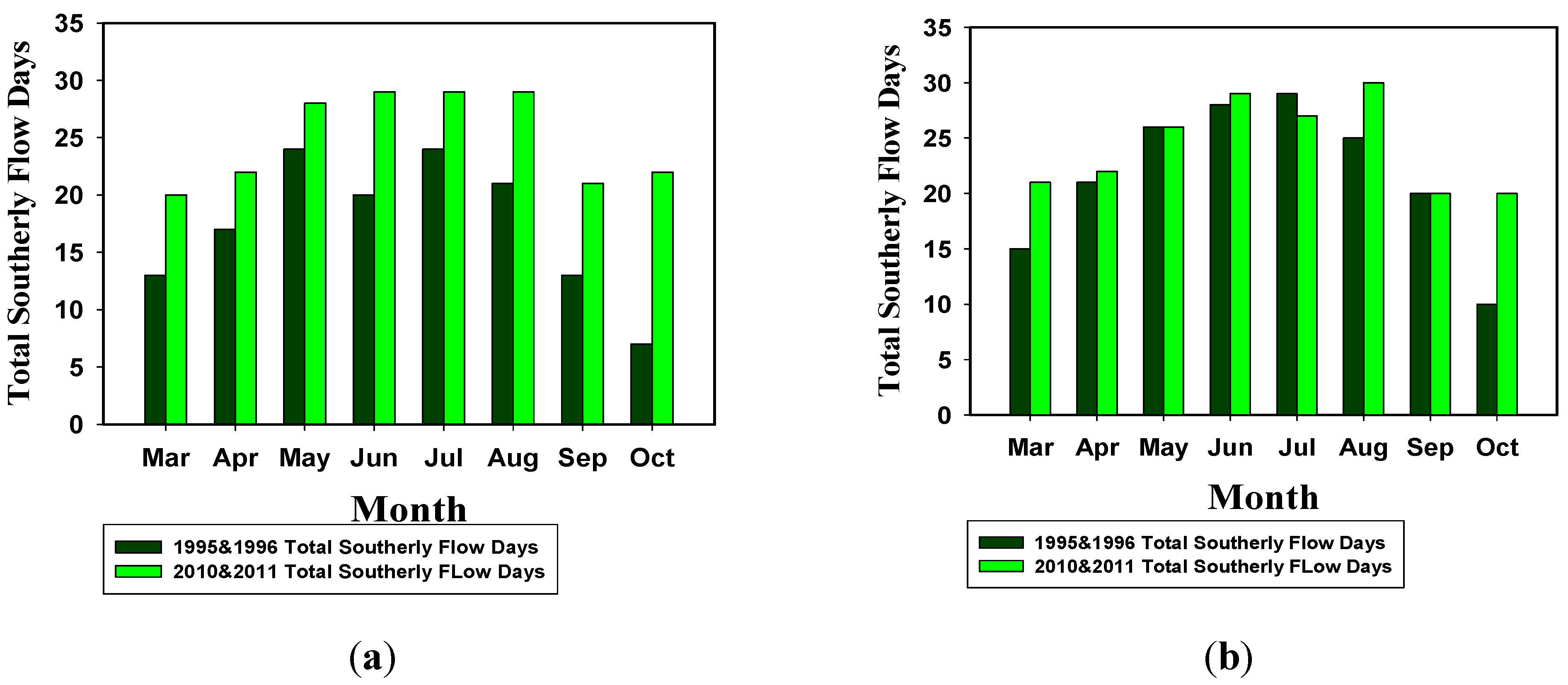
Figure 6 shows that from March to October, total southerly flow days in 2010 and 2011 happened more frequently than that in 1995 and 1996. For both sites, the southerly flow days increase in each month during two sample periods. To the Aldine site, total southerly flow days increase most in March and October, in March, the southerly flow days increased from 13 days to 20 days, and in October, increased from 6 days to 22 days, it is an increase more than a factor of three. To the Galveston site, most increase occurred in October, from 9 days to 20 days, increase by a factor of two.
Figure 6.
Days with southerly flow at Aldine (a) and Galveston (b) average over 1995–1996 (dark green) and 2010–2011 (light green).
Figure 6.
Days with southerly flow at Aldine (a) and Galveston (b) average over 1995–1996 (dark green) and 2010–2011 (light green).
To better understand the southerly flow occurrences at the Aldine and Galveston sites, we analyzed the daily southerly flow hours for the two locations (
Figure 7 and
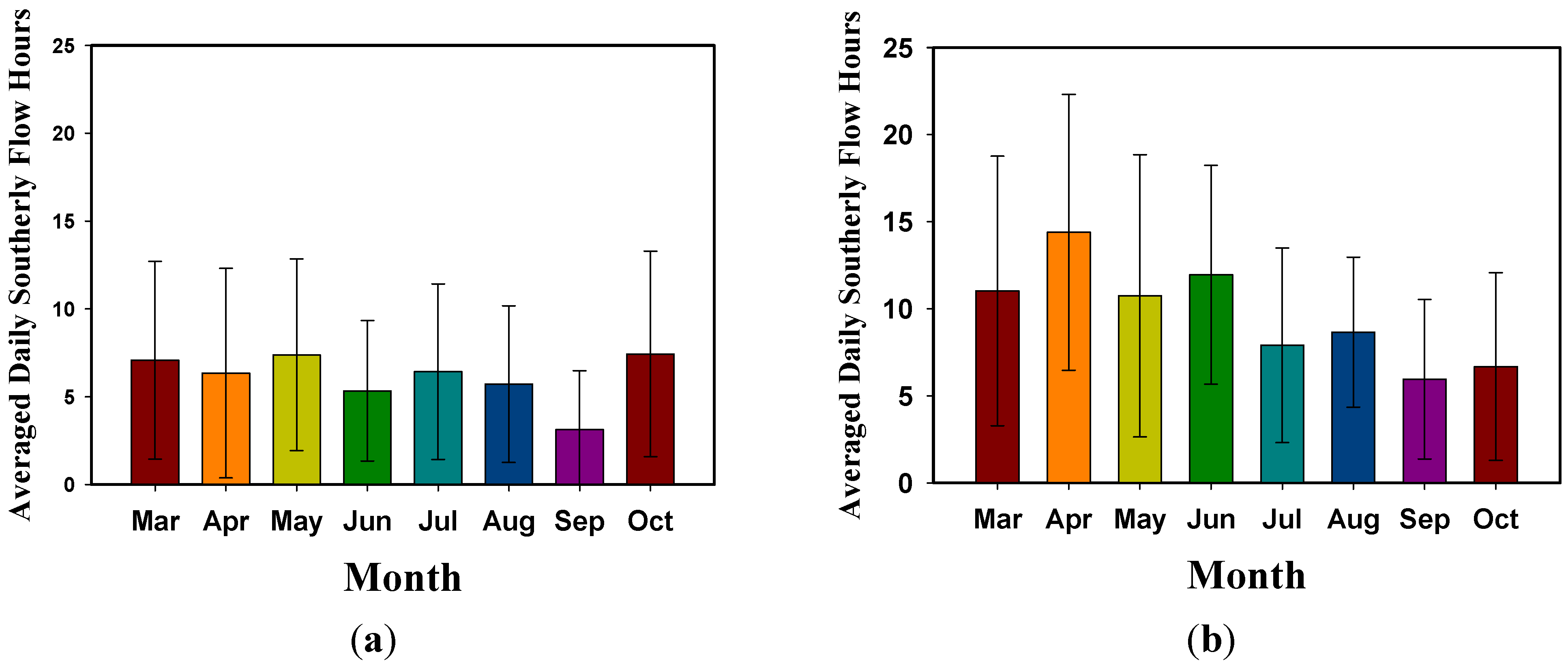
Figure 8). It increased in each month between the two sample periods for both sites. To Aldine site, especially in April (increase from 6 to 15), May (increase from 7 to 11) and June (increase from 5 to 13), daily southerly flow hours increase by a factor of two in average contrasting the two periods. For the Galveston site, most increases occur in April (increase from 5 to 9), August (increase from 6 to 12) and September (increase from 2 to 7). The results for the other sites are presented in the
Supplementary Material (Figures S5 and S6). It is interesting to find out that the daily southerly flow hours have increased the most in the spring and fall seasons at Aldine and Galveston sites. These are the type of trends we would expect with a warming climate [
29,
30].
Figure 7.
Daily southerly flow hours at Aldine during 1995–1996 (a) and 2010–2011 (b).
Figure 7.
Daily southerly flow hours at Aldine during 1995–1996 (a) and 2010–2011 (b).
Figure 8.
Daily southerly flow hours at Galveston during 1995–1996 (a) and 2010–2011 (b).
Figure 8.
Daily southerly flow hours at Galveston during 1995–1996 (a) and 2010–2011 (b).
In order to get a better understanding of the variation in wind direction over past decades, we constructed wind rose graphs for the Houston area. Because there are not enough meteorological data, which can cover the 23 years research time period in the O3 sites we chose, we use the meteorological data from the nearest NCEP monitoring site, and detailed site information is available in the
experimental section. The hourly wind speed and wind direction data are available from National Center for Environmental Protection (NCEP) [
31]. We choose four sites: George Bush Airport (north), Galveston (southeast), William Hobby Airport (near downtown) and David Wayne Hooks Memorial Airport (north).
Figure 9 shows the wind rose for the George Bush Airport site. The other three sites can be found in the
Supporting Materials (Figures S7–S9). We define the frequency of wind direction based on the formula
[
32], where g is the frequency of wind direction N, f is the number of occurrences of the wind direction N for this period and c is the static wind frequency. We choose March to October during 1990~2013 as the time period when southerly flow is most active. Then, the time period was divided into five time intervals and the average for each was calculated. In the rose graph of 1990–1994, general wind directions were from the north (25%), and south and southeast (40%). Wind speeds were generally between 4 and 6 m/s (65%). During 1995–1999 and 2000–2004, major wind directions shifted to the south and southeast. The highest wind speed (8–10 m/s) occurred in the direction of 130°–165°.
During the period 2005–2009, major wind directions were distributed among 160°–195° (32%), which is southerly wind. Wind speeds were in the range of 6–8 m/s (24%) and 13% fell into the range of 8–10 m/s. The frequency and wind speed of the southerly flow increased in contrast to the previous three time intervals. The last interval of 2010–2013, 60% of the wind directions accumulated between 130° and 195°. Specifically, for the directions from 160° to 180°, 30% of the wind speeds were distributed among 6–10 m/s with 5% being in excess of 10 m/s. In summary, the strength of the sea breeze system intensified.
Figure 9.
Wind speed and direction as a function of time for George Bush Airport site.
Figure 9.
Wind speed and direction as a function of time for George Bush Airport site.
2.5. Why an Increase in Southerly Flow?
2.5.1. Land Surface Temperature/Sea Surface Temperature Difference
Both the frequency and wind speed of southerly flow has increased in the most recent two decades, especially during 2000–2013 in the Houston area. As we mentioned previously, the sea breeze usually occurs in the afternoon because of the heat capacity of water is larger than that of soil [
33], which contributes to the temperature differences between land and ocean. To investigate how temperature differences impact southerly flow, we compared land and sea temperatures for the past twenty-three years. Southerly flow occurs mostly from March to October, so we examined hourly land and sea surface temperature data from our study sites. The sea surface temperature (SST) using data from two buoy sites located at the western Gulf of Mexico operated by NOAA National Data Buoy Center [
34].
We used monthly averaged land/sea surface temperature difference in our analysis. We choose the hourly land surface temperature data during 2:00 p.m.–5:00 p.m. (local time) from 1 March to 31 October during 1990–2012, we firstly averaged hourly LST data to get the daily data for each site. Then we averaged the four land sites’ daily data, which is the land surface temperature data for a day. We repeated the processes for each day from March to October during 1990–2012. For the SST, research time period and the method of analyzing was the same with the LST. At last, we employed daily LST data to minus daily SST data, then to calculate the monthly averaged LST-SST temperature difference.
Figure 10 depicts the temperature difference between LST and SST. The largest differences occurred in May and June and these are shown individually in the
Supporting Information (Figure S10). Before the year of 1998, the amplitude between the LST-SST temperature difference was −8 °C to 2 °C, however, a change occurred on September 1998. After the change point, during 1999 to 2012, the amplitude of temperature difference increased to 24 °C (−12 °C to 12 °C), with a high pronounced variability of an unknown cause. The increased variability was not caused by changing out of the measurement devices at any of our study sites. We divide the time period into two stages, the first stage during 1990–1998 and the second stage during 1999–2012. We calculate out the average temperature difference between land and sea for each stage, during 1990–1998, the number is −1.2 °C and during 1999–2012, the average temperature difference is 0.4 °C, an increase of 1.6 °C. The regression trend-line increased from −2 °C to 2 °C during 1990–2013.
Figure 10.
Time series of land surface temperature (LST) minus sea surface temperature (SST) for the Houston area.
Figure 10.
Time series of land surface temperature (LST) minus sea surface temperature (SST) for the Houston area.
For the trend of southerly flow wind speed, as shown in
Figure 11, we analyzed the four land meteorological sites’ wind speed data with wind directions between 160° and 200° and the southerly flow wind speed data are selected from the time period of 2:00 p.m.–5:00 p.m. (local time) from March to October during 1990–2012. After we averaged the four sites’ daily southerly flow wind speed data (average spatially), we calculated average monthly southerly flow wind speeds. The trend line shows monthly average southerly flow wind speed increased by 0.3 m/s from 1990 to 2012. The peak value of the monthly average southerly flow wind speed was 5.8 m/s, which occurred in June of 2012. In summary, the frequency of the southerly flow is intensified and the wind speed of the southerly flow was stable or increased slightly over the last two decades in the Houston area.
Figure 11.
Time series of the monthly averaged wind speed of southerly flow for the Houston area.
Figure 11.
Time series of the monthly averaged wind speed of southerly flow for the Houston area.
2.5.2. Large Scale Atmospheric Circulation
To ascertain what processes caused increased southerly flow in the Houston area we examined the mean sea-level pressure maps for March–October 1995–1996 and 2010–2011. The data were obtained from the National Center for Environmental Prediction [
35] and are shown in
Figure 12. We define the ranges between 120° W–50° W and 50° N–20° S. Comparison of the two time periods indicates that the land surface pressure in Houston during 1995 and 1996 was 1015.5 hPa, during 2010 and 2011 it decreased to 1014.5 hPa. The surface pressure over the Gulf of Mexico, especially around the Houston area, was 1013.5 hPa during 1995 and 1996 and 1015.5 hPa during 2010 and 2011. The terrestrial high-pressure system, which located over Louisiana decreased from 1017.5 hPa to 1016.5 hPa. In summary, surface pressure over the Gulf of Mexico increased while surface pressure over Houston decreased. This pressure difference between land and the Gulf of Mexico probably contributes to increased southerly flow around the Houston area. According to a previous study, eastward displacement of the Bermuda High in 2010 and 2011 may be responsible for reduced summertime O
3 along the U.S. east coast during the past decade [
36].
Figure 12.
National Center for Environmental Prediction (NCEP) reanalysis mean sea-level pressure for March-October in 1995 and 1996 and 2010 and 2011.
Figure 12.
National Center for Environmental Prediction (NCEP) reanalysis mean sea-level pressure for March-October in 1995 and 1996 and 2010 and 2011.
3. Experimental
For the ground-level O3 mixing ratio data, along a south to north transect, we chose four CAMS (continuous ambient monitoring station) sites, which are operated by the Texas Commission on Environmental Quality (TCEQ); they are CAMS 1034 Galveston, CAMS 403 Clinton Ave., CAMS 08 Aldine and CAMS 26 Northwest Harris. The time period for the ground-level O3 mixing ratio begins 1 January, 1990 and ends 31 December, 2013. The format of the O3 data was one-hour averages.
The spatial distribution of our study sites is given in
Figure 13. For the meteorological data, because there are not data, which can cover the 23 years’ research time period in the sites operated by TCEQ, we choose four meteorological monitoring sites closest to the O
3 sites, which are operated by the NOAA National Climatic Data Center, In correspondence with the TCEQ O
3 sites, the meteorology sites are site Galveston (29°16′32.24″ N and 94°50′9.46″ W), William Hobby Airport (29°39′14.79″ N and 95°16′35.81″ W) (Clinton O
3 site), George Bush Intercontinental Airport (29°59′27.13″ N and 95°20′12.70″ W) (Aldine O
3 site), and David Wayne Hooks Memorial Airport (30° 3′31.68″ N and 95°33′2.49″ W) (Northwest Harris O
3 site). The time period for the meteorology data cover the same time period with ground-level O
3 mixing ratio data, which begins 1 January 1990 and ends 31 December 2013. The format of the data is one-hour averages. We analyzed the meteorological factors as local temperature, wind direction, wind speed, pressure, atmospheric circulation and the land-sea breeze. The procedures for the O
3 and CO analysis are provided in [
37]. Sea-level pressure was provided by the NCEP/NCAR reanalysis datasets.
Figure 13.
Spatial distribution of study sites.
Figure 13.
Spatial distribution of study sites.
To the land/sea surface temperature difference, the land surface temperature data is offered by NOAA meteorological sites we choose along the south to north direction (
Figure 12). We choose two buoy sites (27°54′25″ N and 95°21′10″ W, 26°5′29″ N and 93°45′29″ W ) operated by NOAA located in the Gulf of Mexico, which offer the sea surface temperature data.
4. Conclusions
Houston is located close to the Gulf of Mexico and at latitude of 30° N. It is home to a large amount of petroleum industries, which produce and emit chemical precursors for the production of ground-level O3. Because of the critical role meteorology plays in controlling ground-level O3 mixing ratios, we examined it with regard to the rapidly decreasing number of annual O3 exceedances in Houston. Background O3 mixing ratios in Houston are flat or decreasing slightly around 30 ppbv. The exceedance days of 1-h/8-h averaged O3 mixing ratio decrease dramatically from tens of days to only a couple of days annually. A rapid shift occurred around 2000.
Southerly flow has been increasing in the Houston area since at least 1990. Both the frequency and the wind speed of the southerly flow have increased. During 2010~2013, 60% of the wind direction was concentrated in the range of 130°–195°, which is south wind or southeast wind, from the Gulf of Mexico. The cause for increased southerly flow is an increase of nearly 3 °C in LST compared to the SST of the ocean. The net temperature difference between LST and SST increased by a factor of four in May and by a factor of two in June. Before 1999, the range between the maximum and minimum was 12 °C, however, between 1999 and 2012, the range increased to 20 °C, with a pronounced increase in variability. We suspect that this is a worldwide phenomenon.


