Sensitivity of Glacier Runoff to Winter Snow Thickness Investigated for Vatnajökull Ice Cap, Iceland, Using Numerical Models and Observations

 ,
,
Abstract
:1. Introduction
2. Study Site and Observations
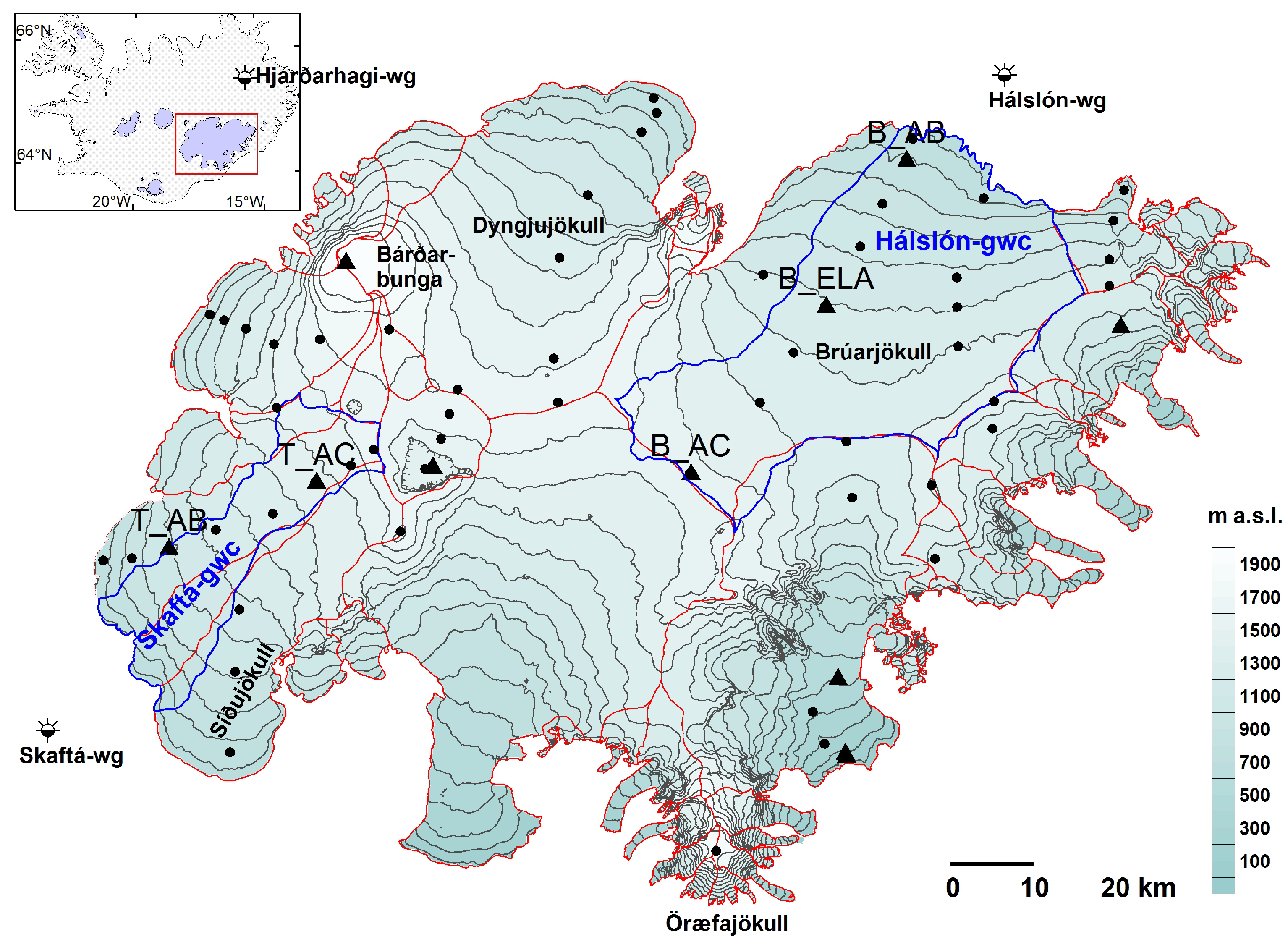
2.1. Study Site
2.2. Energy and Mass Balance
2.3. River Runoff
3. Model Description and Experimental Design
3.1. HIRHAM5 and HARMONIE-AROME
Snow Pack Scheme
3.2. Experiment Design
4. Results
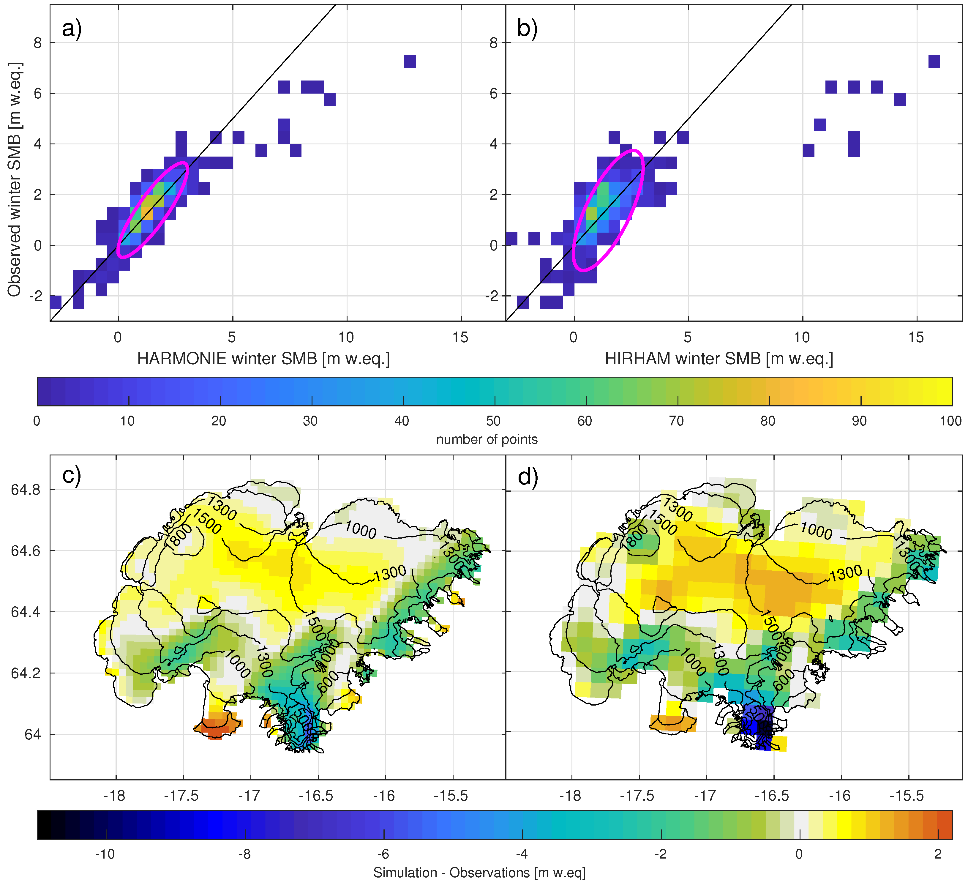
4.1. Evaluation of Model Precipitation
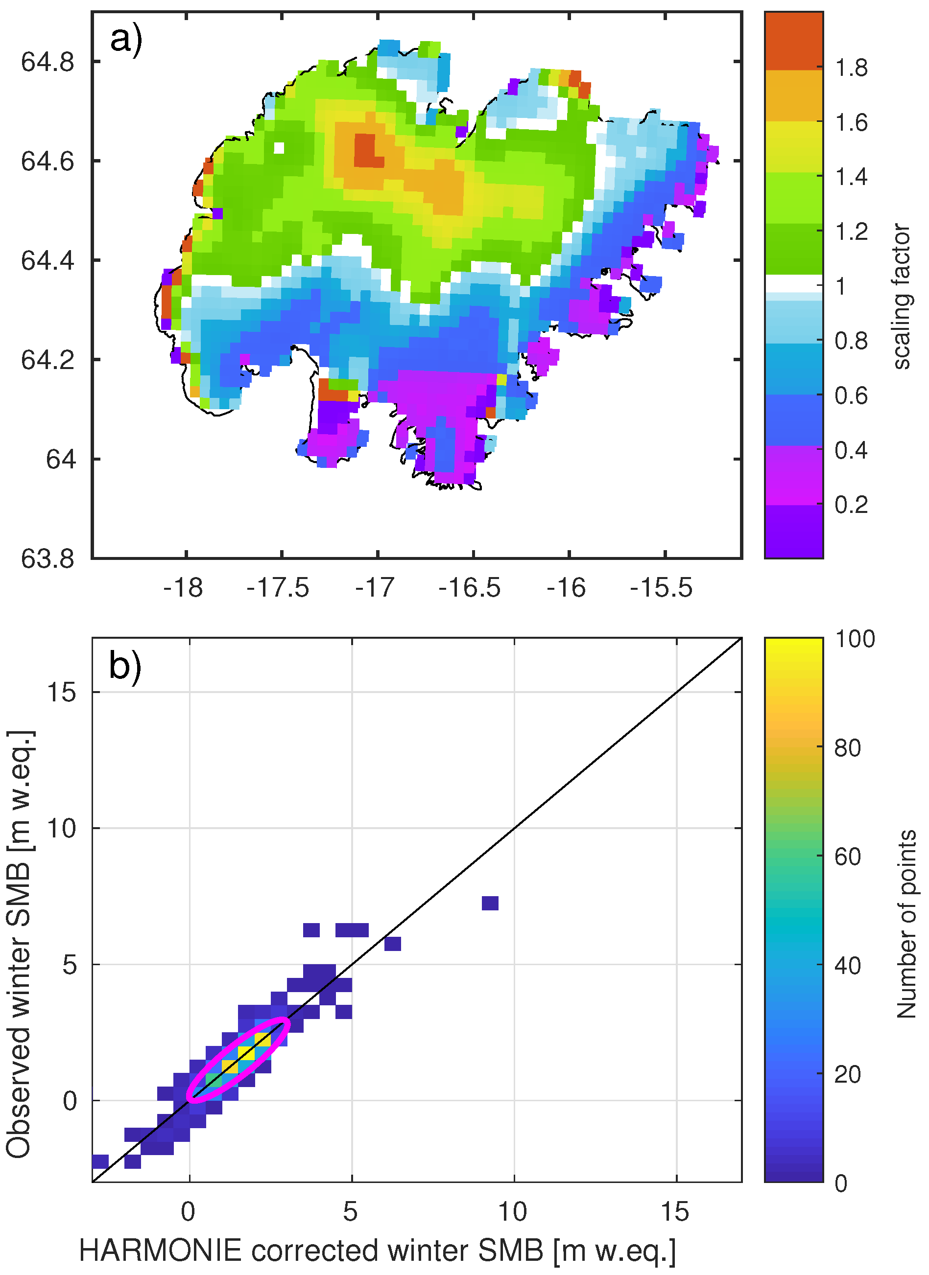
4.2. Accumulation Scaling
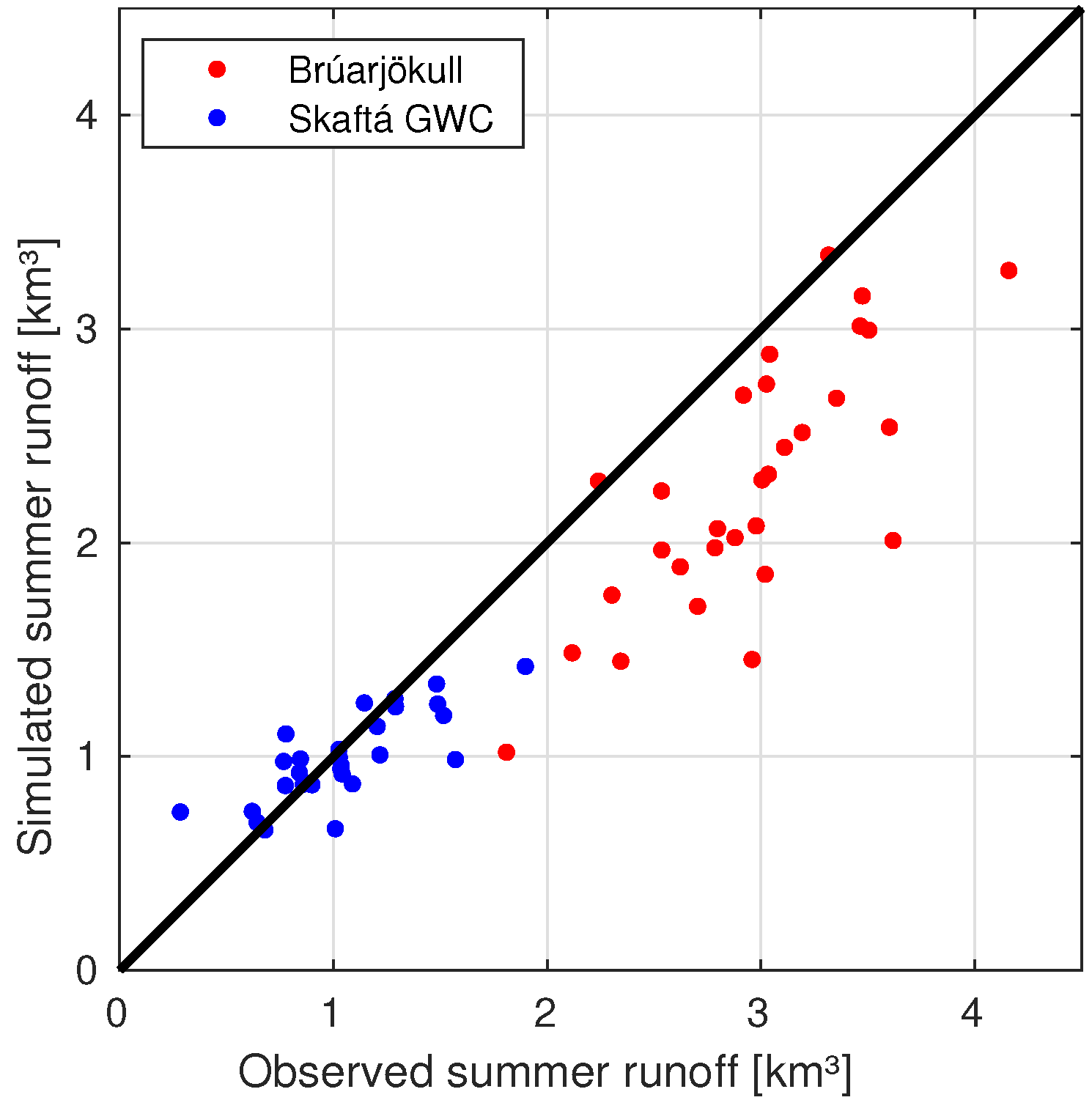
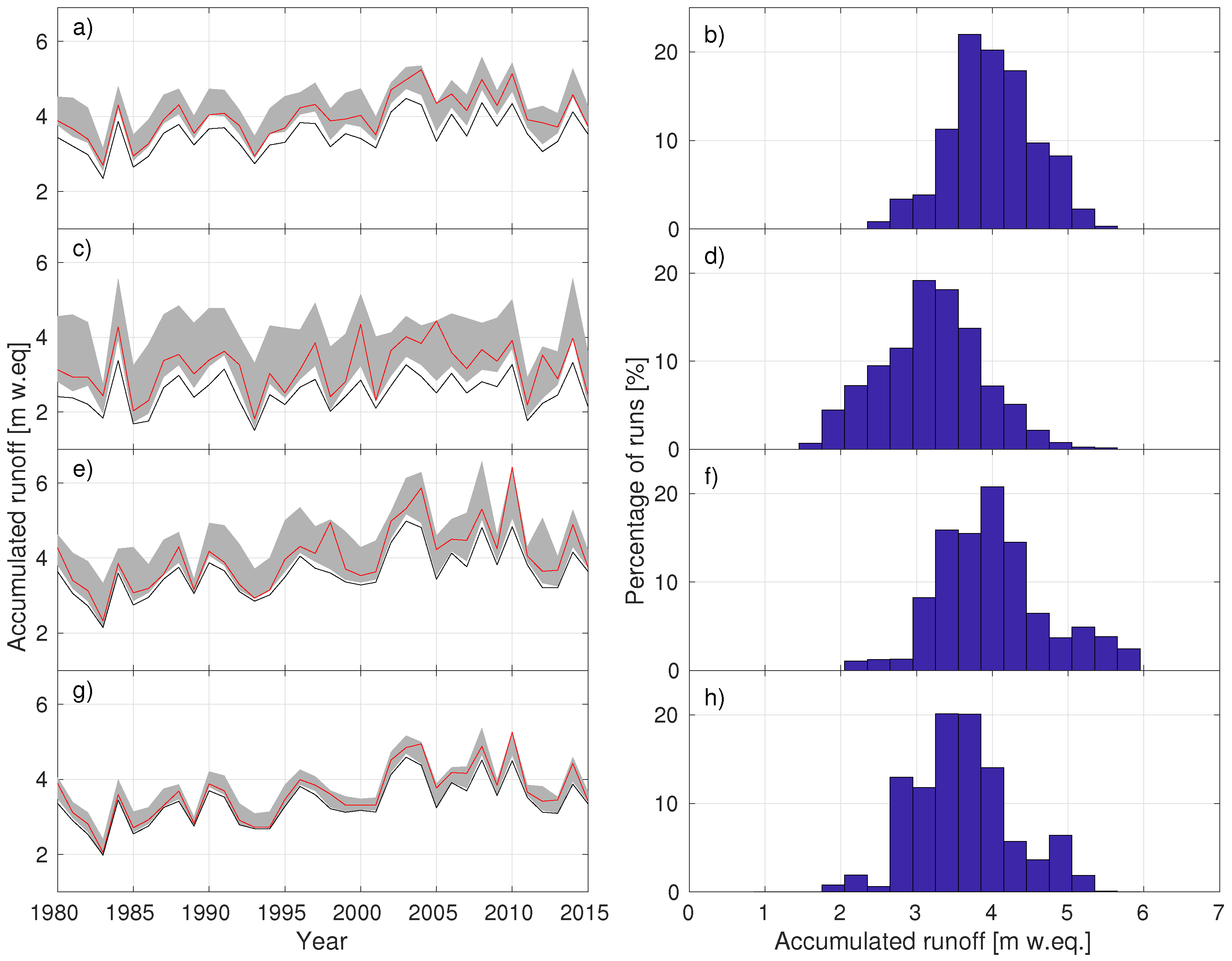
4.3. Comparison to Runoff Measurements
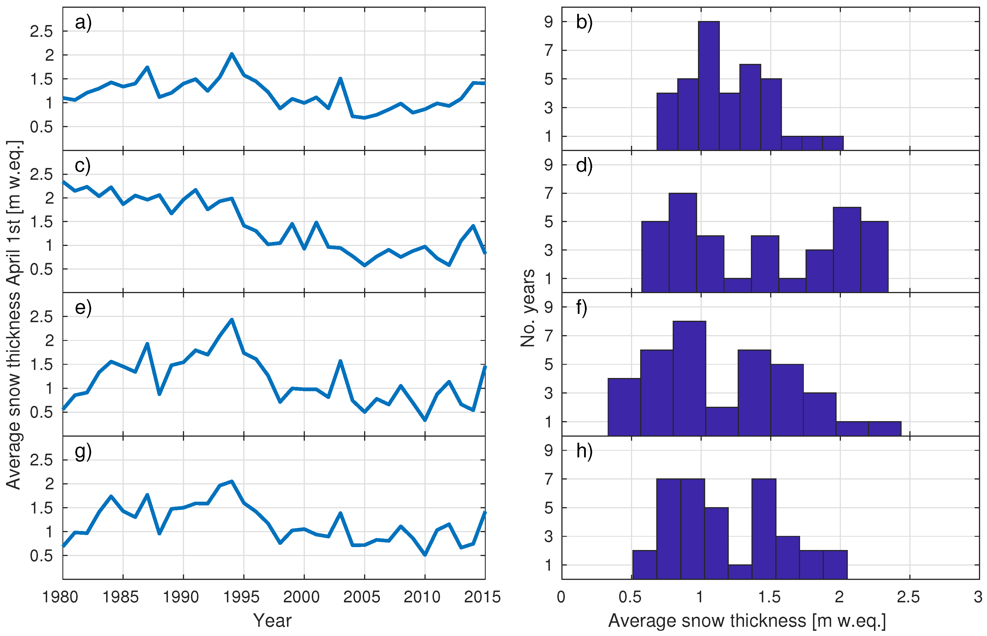
4.4. Snow Thickness on 1 April
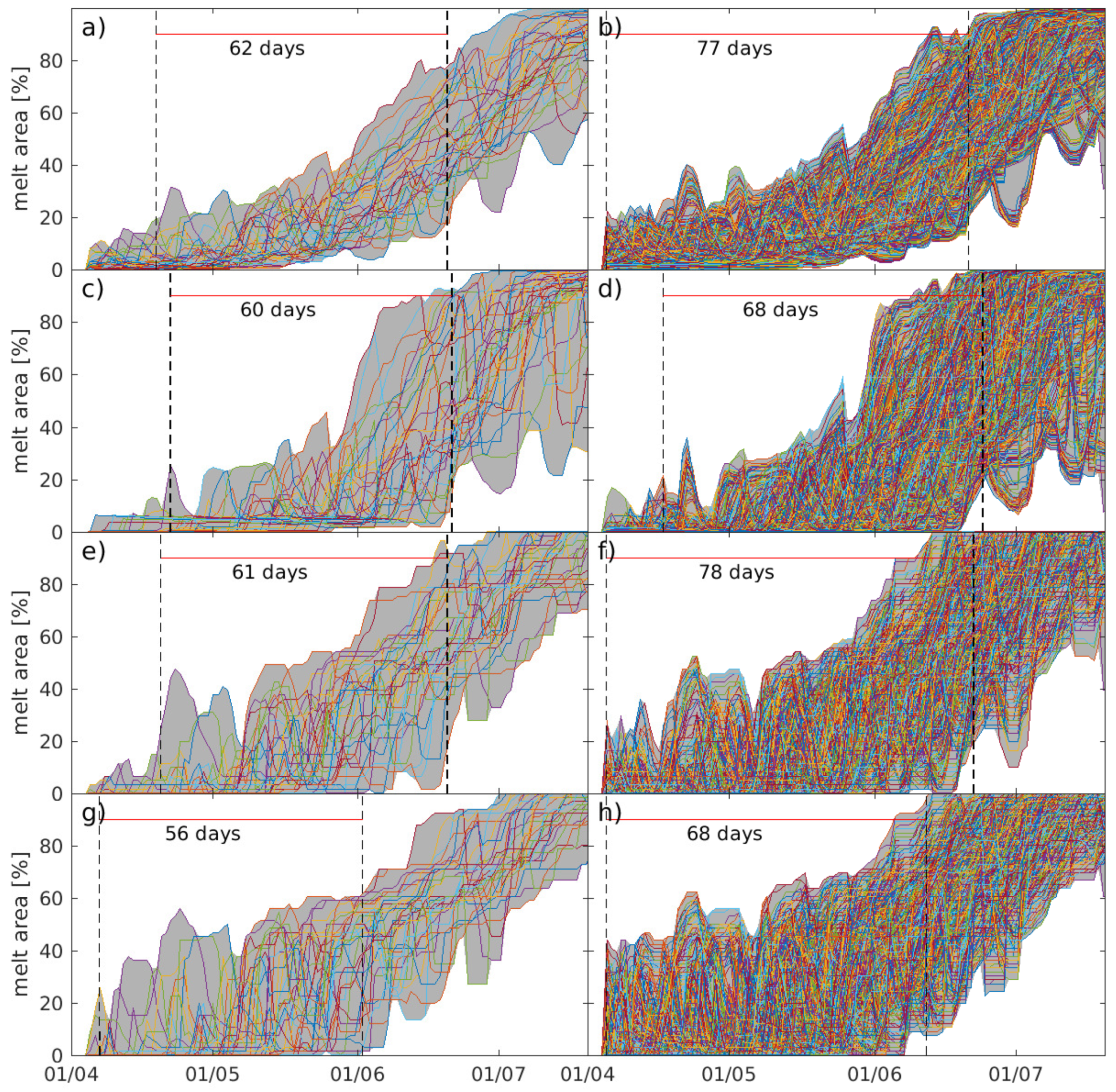
4.5. Sensitivity Runs
5. Discussion
5.1. Modelling of Runoff
5.2. Sensitivity of Runoff to Winter Snow Cover
5.3. Error Sources
6. Conclusions
Author Contributions
Funding
Acknowledgments
Conflicts of Interest
References
- Gregory, J.M.; White, N.J.; Church, J.A.; Bierkens, M.F.P.; Box, J.E.; van den Broeke, M.R.; Cogley, J.G.; Fettweis, X.; Hanna, E.; Huybrechts, P.; et al. Twentieth-Century Global-Mean Sea Level Rise: Is the Whole Greater than the Sum of the Parts? J. Clim. 2013, 26, 4476–4499. [Google Scholar] [CrossRef] [Green Version]
- Jansson, P.; Hock, R.; Schneider, T. The concept of glacier storage: A review. J. Hydrol. 2003, 282, 116–129. [Google Scholar] [CrossRef]
- Huss, M. Present and future contribution of glacier storage change to runoff from macroscale drainage basins in Europe. Water Resour. Res. 2011, 47. [Google Scholar] [CrossRef] [Green Version]
- Kaser, G.; Grosshauser, M.; Marzeion, B. Contribution potential of glaciers to water availability in different climate regimes. Proc. Natl. Acad. Sci. USA 2010, 107, 20223–20227. [Google Scholar] [CrossRef] [PubMed]
- Huss, M.; Hock, R. Global-scale hydrological response to future glacier mass loss. Nat. Clim. Chang. 2018, 8, 135–140. [Google Scholar] [CrossRef] [Green Version]
- Aðalgeirsdóttir, G.; Guðmundsson, S.; Björnsson, H.; Pálsson, F.; Jóhannesson, T.; Hannesdóttir, H.; Sigurðsson, S.T.; Berthier, E. Modelling the 20th and 21st century evolution of Hoffellsjökull glacier, SE-Vatnajökull, Iceland. Cryosphere 2011, 5, 961–975. [Google Scholar] [CrossRef] [Green Version]
- Vaughan, D.G.; Comiso, J.C.; Allison, I.; Carrasco, J.; Kaser, G.; Kwok, R.; Mote, P.; Murray, T.; Paul, F.; Ren, J.; et al. Observations: Cryosphere. In Climate Change 2013: The Physical Science Basis. Contribution of Working Group I to the Fifth Assessment Report of the Intergovernmental Panel on Climate Change; Stocker, T.F., Qin, D., Plattner, G.K., Tignor, M., Allen, S.K., Boschung, J., Nauels, A., Xia, Y., Bex, V., Midgley, P.M., Eds.; Cambridge University Press: Cambridge, UK; New York, NY, USA, 2013. [Google Scholar]
- Björnsson, H.; Pálsson, F.; Guðmundsson, S.; Magnússon, E.; Aðalgeirsdõttir, G.; Jõhannesson, T.; Berthier, E.; Sigurdsson, O.; Thorsteinsson, T. Contribution of Icelandic ice caps to sea level rise: Trends and variability since the Little Ice Age. Geophys. Res. Lett. 2013, 40, 1546–1550. [Google Scholar] [CrossRef] [Green Version]
- Björnsson, H.; Pálsson, F. Icelandic glaciers. Jökull 2008, 58, 365–386. [Google Scholar]
- Schmidt, L.S.; Aðalgeirsdóttir, G.; Guðmundsson, S.; Langen, P.L.; Pálsson, F.; Mottram, R.; Gascoin, S.; Björnsson, H. The importance of accurate glacier albedo for estimates of surface mass balance on Vatnajökull: Evaluating the surface energy budget in a regional climate model with automatic weather station observations. Cryosphere 2017, 11, 1665–1684. [Google Scholar] [CrossRef]
- Gascoin, S.; Guðmundsson, S.; Aðalgeirsdóttir, G.; Pálsson, F.; Schmidt, L.; Berthier, E.; Björnsson, H. Evaluation of MODIS Albedo Product over Ice Caps in Iceland and Impact of Volcanic Eruptions on Their Albedo. Remote Sens. 2017, 9, 399. [Google Scholar] [CrossRef]
- Nawri, N.; Björnsson, H. Surface Air Temperature and Precipitation Trends for Iceland in the 21st Century; Technical Report; Veðurstofa Íslands: Reykjavik, Iceland, 2010. [Google Scholar]
- Greuell, W.; Genthon, C. Modelling land-ice surface mass balance. In Mass Balance of the Cryosphere; Bamber, J.L., Payne, A.J., Eds.; Cambridge University Press: Cambridge, UK, 2004; pp. 117–168. [Google Scholar]
- Meijgaard, E.V.; Ulft, L.H.V.; Bosveld, F.C.; Lenderink, G.; Siebesma, A.P. The KNMI Regional Atmospheric Climate Model RACMO Version 2.1; Technical Report, TR-302; Koninklijk Nederlands Meteorologisch Instituut: De Bilt, The Netherlands, 2008; p. 43. [Google Scholar]
- Skamarock, W.C.; Skamarock, W.C.; Klemp, J.B.; Dudhia, J.; Gill, D.O.; Barker, D.M.; Wang, W.; Powers, J.G. A Description of the Advanced Research WRF Version 3; NCAR Technical Note-475+STR; Scientific Research: Wuhan, China, 2008. [Google Scholar]
- Gallée, H.; Schayes, G. Development of a Three-Dimensional Meso-γ Primitive Equation Model: Katabatic Winds Simulation in the Area of Terra Nova Bay, Antarctica. Mon. Weather Rev. 1994, 122, 671–685. [Google Scholar] [CrossRef]
- Christensen, O.B.; Drews, M.; Christensen, J.H.; Dethloff, K.; Ketelsen, K.; Hebestadt, I.; Rinke, A. The HIRHAM Regional Climate Model Version 5; Technical Report; Danish Meteorological Institute: Copenhagen, Denmark, 2006. [Google Scholar]
- Box, J.E.; Rinke, A. Evaluation of Greenland Ice Sheet Surface Climate in the HIRHAM Regional Climate Model Using Automatic Weather Station Data. J. Clim. 2003, 16, 1302–1319. [Google Scholar] [CrossRef] [Green Version]
- Langen, P.L.; Fausto, R.S.; Vandecrux, B.; Mottram, R.H.; Box, J.E. Liquid Water Flow and Retention on the Greenland Ice Sheet in the Regional Climate Model HIRHAM5: Local and Large-Scale Impacts. Front. Earth Sci. 2017, 4. [Google Scholar] [CrossRef]
- Lenaerts, J.T.M.; Van Den Broeke, M.R. Modeling drifting snow in Antarctica with a regional climate model: 2. Results. J. Geophys. Res. Atmos. 2012, 117. [Google Scholar] [CrossRef] [Green Version]
- Agosta, C.; Fettweis, X.; Datta, R. Evaluation of the CMIP5 models in the aim of regional modelling of the Antarctic surface mass balance. Cryosphere 2015, 9, 2311–2321. [Google Scholar] [CrossRef]
- Giorgi, F.; Jones, C.; Asrar, G.R. Addressing climate information needs at the regional level: The CORDEX framework. World Meteorol. Organ. Bull. 2009, 58, 175. [Google Scholar]
- Nawri, N.; Pálmason, B.; Petersen, N.G.; Björnsson, H.; Þorsteinsson, S. The ICRA Atmospheric Reanalysis Project for Iceland; Technical Report; Veðurstofa Íslands: Reykjavik, Iceland, 2017. [Google Scholar]
- Christensen, J.H.; Boberg, F.; Christensen, O.B.; Lucas-Picher, P. On the need for bias correction of regional climate change projections of temperature and precipitation. Geophys. Rese. Lett. 2008, 35, L20709. [Google Scholar] [CrossRef]
- Hagemann, S.; Chen, C.; Haerter, J.O.; Heinke, J.; Gerten, D.; Piani, C.; Hagemann, S.; Chen, C.; Haerter, J.O.; Heinke, J.; et al. Impact of a Statistical Bias Correction on the Projected Hydrological Changes Obtained from Three GCMs and Two Hydrology Models. J. Hydrometeorol. 2011, 12, 556–578. [Google Scholar] [CrossRef]
- Muerth, M.J.; Gauvin St-Denis, B.; Ricard, S.; Velázquez, J.A.; Schmid, J.; Minville, M.; Caya, D.; Chaumont, D.; Ludwig, R.; Turcotte, R. On the need for bias correction in regional climate scenarios to assess climate change impacts on river runoff. Hydrol. Earth Syst. Sci. 2013, 17, 1189–1204. [Google Scholar] [CrossRef] [Green Version]
- Gudmundsson, L.; Bremnes, J.B.; Haugen, J.E.; Engen-Skaugen, T. Technical Note: Downscaling RCM precipitation to the station scale using statistical transformations—A comparison of methods. Hydrol. Earth Syst. Sci. 2012, 16, 3383–3390. [Google Scholar] [CrossRef]
- Switanek, M.B.; Troch, P.A.; Castro, C.L.; Leuprecht, A.; Chang, H.I.; Mukherjee, R.; Demaria, E.M.C. Scaled distribution mapping: A bias correction method that preserves raw climate model projected changes. Earth Syst. Sci. 2017, 215194, 2649–2666. [Google Scholar] [CrossRef]
- Bengtsson, L.; Andrae, U.; Aspelien, T.; Batrak, Y.; Calvo, J.; de Rooy, W.; Gleeson, E.; Hansen-Sass, B.; Homleid, M.; Hortal, M.; et al. The HARMONIE–AROME Model Configuration in the ALADIN–HIRLAM NWP System. Mon. Weather Rev. 2017, 145, 1919–1935. [Google Scholar] [CrossRef]
- Xu, M.; Yan, M.; Kang, J.; Ren, J. Comparative studies of glacier mass balance and their climatic implications in Svalbard, Northern Scandinavia, and Southern Norway. Environ. Earth Sci. 2012, 67, 1407–1414. [Google Scholar] [CrossRef]
- Engelhardt, M.; Schuler, T.V.; Andreassen, L.M. Sensitivities of glacier mass balance and runoff to climate perturbations in Norway. Ann. Glaciol. 2015, 56, 79–88. [Google Scholar] [CrossRef] [Green Version]
- De Woul, M.; Hock, R. Static mass-balance sensitivity of Arctic glaciers and ice caps using a degree-day approach. Ann. Glaciol. 2005, 42, 217–224. [Google Scholar] [CrossRef]
- Gudmundsson, M.T.; Thordarson, T.; Höskuldsson, Á.; Larsen, G.; Björnsson, H.; Prata, F.J.; Oddsson, B.; Magnússon, E.; Högnadóttir, T.; Petersen, G.N.; et al. Ash generation and distribution from the April–May 2010 eruption of Eyjafjallajökull, Iceland. Sci. Rep. 2012, 2, 572. [Google Scholar] [CrossRef] [PubMed] [Green Version]
- Oerlemans, J.; Björnsson, H.; Kuhn, M.; Obleitner, F.; Palsson, F.; Smeets, C.; Vugts, H.F.; Wolde, J.D. Glacio-Meteorological Investigations On Vatnajökull, Iceland, Summer 1996: An Overview. Bound.-Layer Meteorol. 1999, 92, 3–24. [Google Scholar] [CrossRef]
- Guðmundsson, S.; Björnsson, H.; Pálsson, F.; Haraldsson, H.H. Energy balance of Brúarjökull and circumstances leading to the August 2004 floods in the river Jökla, N-Vatnajökull. Jökull 2006, 55, 121–138. [Google Scholar]
- Björnsson, H.; Palsson, F.; Guðmundsson, M.T. Afkoma, Hreyfing og Afrennsli á Vestan-og Norðanverðum Vatnajokli Jökulárin 1992–1993 og 1993 (Mass Balance, Movement and Runoff on Western and Northern Vatnajökull Hydrological Years 1992–1993 and 1993–1994); Technical Report; University of Iceland: Reykjavik, Iceland, 1995. [Google Scholar]
- Landsvirkjun. Wiski Database 28.11.2017—M00328; WISKI: Roseville, CA, USA, 2017. [Google Scholar]
- Snorrason, A.; Gunnarsson, A.; Jónsson, P.; Einarsson, K.; Sigurðsson, O. Summary of Available Hydrological Information in the Jökulsá á Deal and Jökulsá í Fljótsdal Basins, Iceland; Technical Report; Orkustofnun: Reykjavik, Iceland, 1998. [Google Scholar]
- Icelandic Meteorological Office Database. Discharge Data 1986–2016; Icelandic Meteorological Office Database: Reykjavik, Iceland, 2017. [Google Scholar]
- Hardarðóttir, J.; Snorrason, A. Sediment monitoring of glacial rivers in Iceland: New data on bed load transport. Hydrol. Sci. J. 2003, 283, 154–163. [Google Scholar]
- Schulla, J. Model Description WaSiM (Water Balance Simulation Model); Technical Report; Hydrology Software Consulting J. Schulla: Zurich, Switzerland, 2017. [Google Scholar]
- Jónsdóttir, J.F. A runoff map based on numerically simulated precipitation and a projection of future runoff in Iceland / Une carte d’écoulement basée sur la précipitation numériquement simulée et un scénario du futur écoulement en Islande. Hydrol. Sci. J. 2008, 53, 100–111. [Google Scholar] [CrossRef]
- Einarsson, B. Improving Groundwater Representation and the Parameterization of Glacial Melting and Evapotranspiration in Applications of the WaSiM Hydrological Model within Iceland Improving Groundwater Representation and the Parameterization of Glacial Melting and Eva; Technical Report; Icelandic Meteorological Office: Reykjavi, Iceland, 2010.
- Björnsson, H. The cause of jökulhlaups in the Skaftá-river, Vatnajökull. Jökull 1977, 27, 71–78. [Google Scholar]
- Björnsson, H. Hydrology of Ice Caps in Volcanic Regions; Societas Scientarium Islandica, University of Iceland: Reykjavik, Iceland, 1988; p. 139. [Google Scholar]
- Eerola, K. About the performance of HIRLAM version 7.0. HIRLAM Newsl. 2006, 51, 93–102. [Google Scholar]
- Roeckner, E.; Bäuml, G.; Bonaventura, L.; Brokopf, R.; Esch, M.; Giorgetta, M.; Hagemann, S.; Kirchner, I.; Kornblueh, L.; Manzini, E.; et al. The Atmospheric General Circulation Model ECHAM 5 PART I: Model Description; Technical Report 349; MPI für Meteorologie: Hamburg, Germany, 2003. [Google Scholar]
- Dee, D.P.; Uppala, S.M.; Simmons, A.J.; Berrisford, P.; Poli, P.; Kobayashi, S.; Andrae, U.; Balmaseda, M.A.; Balsamo, G.; Bauer, P.; et al. The ERA-Interim reanalysis: Configuration and performance of the data assimilation system. Q. J. R. Meteorol. Soc. 2011, 137, 553–597. [Google Scholar] [CrossRef]
- Stendel, M.; Christensen, J.H.; Petersen, D. High-Arctic Ecosystem Dynamics in a Changing Climate. In Advances in Ecological Research; Elsevier: Amsterdam, The Netherlands, 2008; Volume 40, pp. 13–43. [Google Scholar]
- Lucas-Picher, P.; Wulff-Nielsen, M.; Christensen, J.H.; Aðalgeirsdóttir, G.; Mottram, R.H.; Simonsen, S.B. Very high resolution regional climate model simulations over Greenland: Identifying added value. J. Geophys. Res. 2012, 117, 2108. [Google Scholar] [CrossRef]
- Langen, P.L.; Mottram, R.H.; Christensen, J.H.; Boberg, F.; Rodehacke, C.B.; Stendel, M.; van As, D.; Ahlstrøm, A.P.; Mortensen, J.; Rysgaard, S.; et al. Quantifying energy and mass fluxes controlling godthåbsfjord freshwater input in a 5-km simulation (1991–2012). J. Clim. 2015, 28, 3694–3713. [Google Scholar] [CrossRef]
- Rae, J.G.L.; Aðalgeirsdóttir, G.; Edwards, T.L.; Fettweis, X.; Gregory, J.M.; Hewitt, H.T.; Lowe, J.A.; Lucas-Picher, B.; Mottram, R.H.; Payne, A.J.; et al. Greenland ice sheet surface mass balance: Evaluating simulations and making projections with regional climate models. Cryosphere 2012, 6, 1275–1294. [Google Scholar] [CrossRef]
- Seity, Y.; Brousseau, P.; Malardel, S.; Hello, G.; Bénard, P.; Bouttier, F.; Lac, C.; Masson, V.; Seity, Y.; Brousseau, P.; et al. The AROME-France Convective-Scale Operational Model. Mon. Weather Rev. 2011, 139, 976–991. [Google Scholar] [CrossRef]
- Schaaf, C.; Wang, Z. MCD43A3 MODIS/Terra+Aqua BRDF/Albedo Daily L3 Global—500 m V006. NASA EOSDIS Land Process. DAAC 2015. [Google Scholar] [CrossRef]
- Guðmundsson, M.T. Mass balance and precipitation on the summit plateau of Öræfajökull, SE-Iceland. Jökull 2000, 48, 49–54. [Google Scholar]
- Belart, J.M.; Magnússon, E.; Berthier, E.; Gunnarsson, A.Þ.; Pálsson, F.; Aðalgeirsdóttir, G.; Björnsson, H. Spatially distributed mass balance of Icelandic glaciers and ice caps, 1945–present. Trends and link with climate. Earth Syst. Sci. Data 2018, in press. [Google Scholar]
- Guðmundsson, S.; Björnsson, H.; Pálsson, F.; Haraldsson, H.H. Comparison of energy balance and degree-day models of summer ablation on the Langjökull ice cap, SW-Iceland. Jökull 2009, 59, 1–18. [Google Scholar]
- Bellaire, S.; Jamieson, B. Forecasting the formation of critical snow layers using a coupled snow cover and weather model. Cold Reg. Sci. Technol. 2013, 94, 37–44. [Google Scholar] [CrossRef]
- Vionnet, V.; Dombrowski-Etchevers, I.; Lafaysse, M.; Quéno, L.; Seity, Y.; Bazile, E.; Vionnet, V.; Dombrowski-Etchevers, I.; Lafaysse, M.; Quéno, L.; et al. Numerical Weather Forecasts at Kilometer Scale in the French Alps: Evaluation and Application for Snowpack Modeling. J. Hydrometeorol. 2016, 17, 2591–2614. [Google Scholar] [CrossRef]
- Larsen, K.M.H.; Gonzalez-Pola, C.; Fratantoni, P.; Beszczynska-Möller, A.; Hughes, S.L. ICES Report on Ocean Climate 2015. ICES Coop. Res. Rep. 2016, 331, 79. [Google Scholar]
- Jones, P.D.; Lister, D.H.; Osborn, T.J.; Harpham, C.; Salmon, M.; Morice, C.P. Hemispheric and large-scale land-surface air temperature variations: An extensive revision and an update to 2010. J. Geophys. Res. Atmos. 2012, 117. [Google Scholar] [CrossRef] [Green Version]
- Dragosics, M.; Meinander, O.; Jónsdóttír, T.; Dürig, T.; De Leeuw, G.; Pálsson, F.; Dagsson-Waldhauserová, P.; Thorsteinsson, T. Insulation effects of Icelandic dust and volcanic ash on snow and ice. Arab. J. Geosci. 2016, 9, 126. [Google Scholar] [CrossRef]
- Wittmann, M.; Groot Zwaaftink, C.D.; Steffensen Schmidt, L.; Guðmundsson, S.; Pálsson, F.; Arnalds, O.; Björnsson, H.; Thorsteinsson, T.; Stohl, A. Impact of dust deposition on the albedo of Vatnajökull ice cap, Iceland. Cryosphere 2017, 11, 741–754. [Google Scholar] [CrossRef]
- Fountain, A.G. Effect of snow and firn hydrology on the physical and chemical characteristics of glacier runoff. Hydrol. Process. 1996, 10, 509–521. [Google Scholar] [CrossRef]
- Nienow, P.; Hubbard, B. Surface and Englacial Drainage of Glaciers and Ice Sheets. In Encyclopedia of Hydrological Sciences; John Wiley & Sons, Ltd.: Chichester, UK, 2005. [Google Scholar]
- Banwell, A.; Hewitt, I.; Willis, I.; Arnold, N. Moulin density controls drainage development beneath the Greenland ice sheet. J. Geophys. Res. Earth Surf. 2016, 121, 2248–2269. [Google Scholar] [CrossRef] [Green Version]
- Flowers, G.E.; Björnsson, H.; Pálsson, F. New insights into the subglacial and periglacial hydrology of Vatnajökull, Iceland, from a distributed physical model. J. Glaciol. 2003, 49, 257–270. [Google Scholar] [CrossRef]
Sample Availability: The ICRA HARMONIE-AROME runs over Iceland, as well as the Skaftá runoff time series and WaSiM model results, can be acquired by contacting the Icelandic Meteorological office. The runoff measurements from Hálslón and Hjarðarhagi can be acquired by contacting the Icelandic power company Landsvirkjun. Measurements from automatic weather stations and from in situ mass balance surveys are partially owned by the National Power Company of Iceland and are therefore not publicly available at this time. |


| Components | Observed Value | HIR Diff | HAR Diff | HIR RMSE | HAR RMSE | HIR r | HAR r |
|---|---|---|---|---|---|---|---|
| Winter SMB (m w.eq.) | 1.5 | 0.04 | −0.07 | 1.2 | 0.6 | 0.82 | 0.87 |
| SW↓ (W m) | 224.7 | −32.0 | 2.4 | 67.2 | 49.9 | 0.80 | 0.87 |
| LW↓ (W m) | 283.2 | −9.0 | −12.8 | 22.7 | 22.1 | 0.80 | 0.87 |
| Turbulent fluxes (W m) | 27.6 | −6.5 | −8.9 | 32 | 28.8 | 0.43 | 0.46 |
| Glacial Catchment | Period | Mean Observed Summer Runoff (km) | Model-Obs (km) | RMSE | r |
|---|---|---|---|---|---|
| Skaftá GWC | 1986–2015 | 1.06 | −0.07 | 0.22 | 0.78 |
| Bruárjökull | 1980–2015 | 2.9 | −0.6 | 0.74 | 0.89 |
| Mean SR (m w.eq.) | Min SR (m w.eq.) | Max SR (m w.eq.) | SR Diff (%) | Mean TS (m w.eq.) | TS Diff (%) | |||
|---|---|---|---|---|---|---|---|---|
| Vatnajökull | 4.0 | 3.8 | 4.5 | 19.4 | 0.17 | 0.54 | 3.5 | 13.6 |
| Bruárjökull | 3.2 | 2.8 | 4.3 | 53.3 | 0.31 | 0.61 | 2.5 | 27.2 |
| Siðujökull | 4.0 | 3.7 | 4.7 | 26.8 | 0.23 | 0.70 | 3.6 | 11.8 |
| Skaftá GWC | 3.6 | 3.4 | 3.9 | 13.6 | 0.12 | 0.64 | 3.4 | 7.4 |
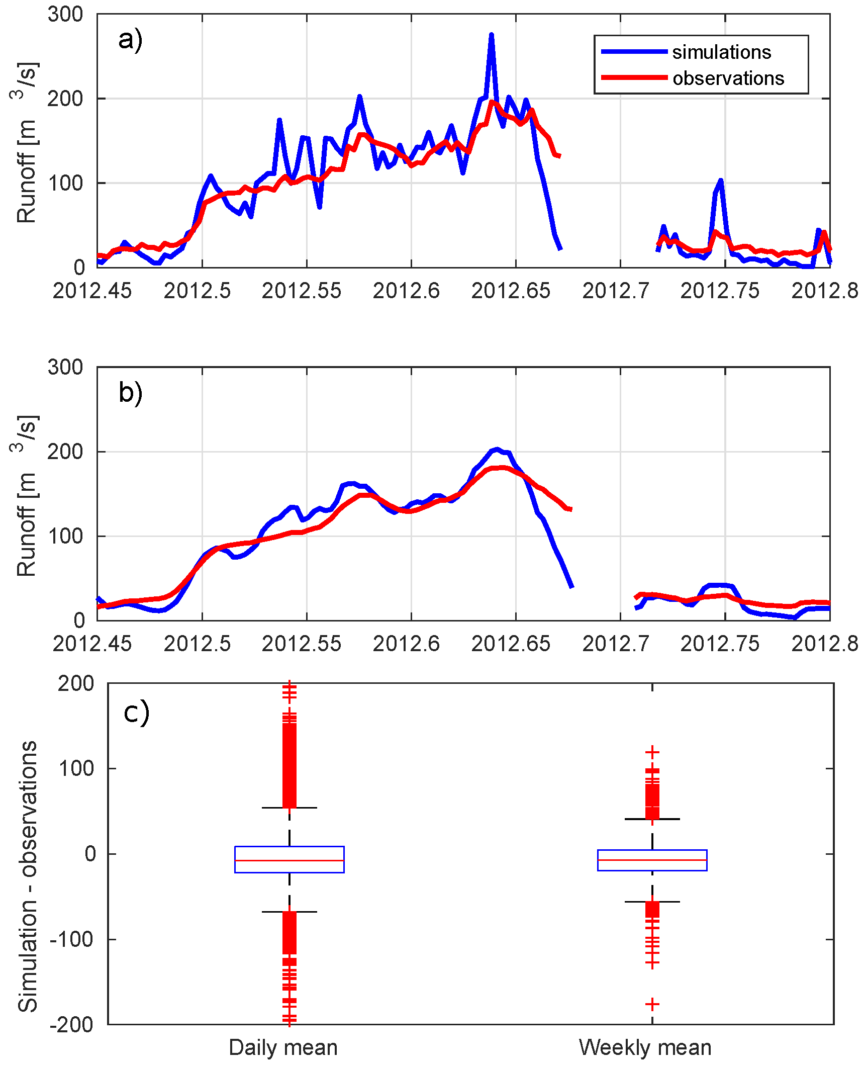
| Glacial Catchment | Period | Timescale | Mean Obs Runoff (m/s) | Model-Obs (m/s) | RMSE (m/s) | r | NSE |
|---|---|---|---|---|---|---|---|
| Skaftá GWC | 1986–2015 | Daily | 58.0 | −4.1 | 41.1 | 0.75 | 0.44 |
| 1-day shift | 38.9 | 0.78 | 0.50 | ||||
| Weekly | 32.0 | 0.82 | 0.66 | ||||
| Brúarjökull | 1980–2015 | Daily | 183.9 | −83.4 | 144.9 | 0.73 | 0.42 |
| 1-day shift | 137.6 | 0.77 | 0.51 | ||||
| Weekly | 121.7 | 0.84 | 0.59 |
© 2018 by the authors. Licensee MDPI, Basel, Switzerland. This article is an open access article distributed under the terms and conditions of the Creative Commons Attribution (CC BY) license (http://creativecommons.org/licenses/by/4.0/).
Share and Cite
Schmidt, L.S.; Langen, P.L.; Aðalgeirsdóttir, G.; Pálsson, F.; Guðmundsson, S.; Gunnarsson, A. Sensitivity of Glacier Runoff to Winter Snow Thickness Investigated for Vatnajökull Ice Cap, Iceland, Using Numerical Models and Observations. Atmosphere 2018, 9, 450. https://doi.org/10.3390/atmos9110450
Schmidt LS, Langen PL, Aðalgeirsdóttir G, Pálsson F, Guðmundsson S, Gunnarsson A. Sensitivity of Glacier Runoff to Winter Snow Thickness Investigated for Vatnajökull Ice Cap, Iceland, Using Numerical Models and Observations. Atmosphere. 2018; 9(11):450. https://doi.org/10.3390/atmos9110450
Chicago/Turabian StyleSchmidt, Louise Steffensen, Peter L. Langen, Guðfinna Aðalgeirsdóttir, Finnur Pálsson, Sverrir Guðmundsson, and Andri Gunnarsson. 2018. "Sensitivity of Glacier Runoff to Winter Snow Thickness Investigated for Vatnajökull Ice Cap, Iceland, Using Numerical Models and Observations" Atmosphere 9, no. 11: 450. https://doi.org/10.3390/atmos9110450