1. Introduction
The atmospheric moisture field presents variation of high and low frequencies. These frequencies depend directly on the heating of the terrestrial surface and indirectly on some variability patterns of low frequency by teleconnection [
1,
2]. In addition, the space field presents variability associated with wind, topography and surfaces types. Wind changes moisture by advectives or recycling processes. Topography is responsible for large amount of water vapor moving windward of the mountain, and small amount moving downwind. The plane and coastal surfaces present a larger storage of water vapor than continental areas [
3,
4].
The numerical representation of the atmospheric moisture field involving these characteristics still presents a challenge in modeling. Although the models of Numerical Weather Prediction (NWP) are quite useful to spatially characterize the behavior of the atmospheric moisture, they are deficient at physically representing all the involved processes. Due to temporal and spatial discretization applied in this model, several of these processes require a parameterization that has been developed for simulations of the atmosphere. A portion of the imprecision of these simulations is from the uncertainties contained in the observations [
5,
6].
Statistical combination of atmospheric moisture observations with the predicted fields using a numerical model in a optimization methodology is denominated data assimilation. This strategy can be the best solution to obtain a more realistic space representation of atmospheric moisture. The observations are introduced in the cycles of numerical prediction to minimize the increase of error during the model integration in a feedback process. This generates initial conditions that are influenced by observation to better represent the physical reality, considering the deficiency of the used model. This cyclical procedure is one of the most important characteristics of the data assimilation process because it allows the concatenation of the contribution of the observations in different steps in the process of integration of the model [
7]. This minimizes the deficiency in the collected data and the atmospheric modeling.
The efficiency of the data assimilation process in the moisture fields is directly related to the choice of the atmospheric moisture control variable employed in the process of uncertainties minimization. The moisture control variable is correlated with other variables, which promote modification by moisture observation not only in the moisture field, but also in the fields of the correlated variable. The suitable choice of this control variable permits us to minimize the contamination of the moisture observation uncertainty to other variables measured and predicted with larger precision, e.g., temperature. Furthermore, the moisture control variable has an important impact on the total precipitable water predicted by the model. This has implications for the quality of the precipitation forecast, which is the most important NWP product for human activities.
Several previous studies have investigated the impact of a suitable choice of moisture control variable in the data assimilation process [
8,
9,
10]. Using a Physical-Space Statistical Analysis System (PSAS), Dee et al. [
9] observed the impact on the moisture initial conditions when different variables (such as mixing ratio, specific moisture, logarithm of specific moisture, relative moisture and pseudo-relative humidity) were chosen as moisture control variable of the atmospheric moisture fields.
Lorenc et al. [
11] showed that the preservation of the relative humidity when humidity observations are not available can be advantageous to global data assimilation system at the UK Met Office, because the cloud parameterization in the model is directly associated with relative humidity. However, if the model has cold bias in the stratosphere, the increase in the values of the observed temperature causes spurious humidity accumulation, which is condensed in the stratosphere by the model. To contain the increase this stratospheric humidity, it is possible to introduce an artificial variable or to use pseudo-relative humidity as moisture control variable. Pseudo-relative humidity is dependent on the background temperature and is consequently related to all of the processes of correction of the model trajectory inside of the cycle of data assimilation [
9].
The correct choice of the moisture moisture control variable is very important. It is necessary to consider the skill of the model, the availability of humidity observation systems and the data assimilation method. Different centers use different atmospheric moisture control variables; the Center for Weather Forecast and Climate Studies (CPTEC) from National Institute for Space Research (INPE) uses the normalized relative humidity. However, the current data assimilation system (GSI, Gridpoint Statistical Interpolation) permits us to explore the pseudo-relative humidity as moisture control variable [
9,
12].
The objective of this work is to evaluate the sensitivity of the initial conditions and forecasts in the basic state and atmospheric moisture fields as a function of the selected moisture control variable in the data assimilation process. To do this, it is necessary to accomplish simulations in cyclical experiments of assimilation using GSI coupled in the CPTEC/INPE model. In this case, the normalized relative humidity and pseudo-relative humidity are used as moisture control variables in the data assimilation.
In
Section 2, the methodology is presented. An emphasis is placed on the GSI and CPTEC/INPE model, the experiment designer and the evaluation strategy employed here. We also prioritize a discussion about which moisture control variables are available in the process of data assimilation implemented in GSI. In
Section 3, the results are presented and described. In
Section 4, the conclusions and final comments are discussed.
2. Materials and Methods
The model used in this study was Brazilian Global Model from CPTEC/INPE, T299L64, with a horizontal resolution of approximately 44 km near the equator. The equations are written in spectral form and the equations of horizontal motion are transformed into vorticity and divergence equations. The initial condition undergoes an initialization process using the normal modes of the linearized model of a basic state at rest and considering temperature only as a vertical function [
13].
The Brazilian Global Model uses the Simple Biosphere Model (SSiB) to represent the terrestrial surface [
14]. Dynamic processes and physical parameterizations involve the Kuo scheme for deep convection [
15], the Tiedtke for shallow convection, Mellhor and Yamada closure scheme for the vertical diffusion in the planetary boundary layer, and the biharmonic-type diffusion for the horizontal diffusion.
The surface variables (soil surface temperature, soil moisture, surface albedo and snow thickness) are introduced at the beginning of integration with the climatological values and adjusted throughout the integration. More information about the configuration of the Brazilian Global Model can be found in Cavalcanti et al. [
16].
The Grid point Statistical Interpolation (GSI, [
17]) system implemented at CPTEC/INPE uses the previous 6-h forecast from Brazilian Global Model as background. Then, a new estimate of the atmospheric state (analysis) is required every 6 h to initialize the Brazilian Global Model that covers the 6-h data window centered on the analysis time. The analyses are used as the initial conditions for subsequent forecasts and the cycle continues.
The GSI system is a three-dimensional (3-D) variational data assimilation (3DVAR) method. The solution of 3D variational data assimilation is sought as the minimum of the following cost function [
17,
18].
where
x is the state vector composed of the model variables at every grid point,
x is the background state vector,
y is the vector of observations, and
H is the non-linear observation operator, which provides a map from the gridded model variables to the observation locations. The
J term contains
R, the observational error covariance matrix. The
J term contains
B, the background error covariance matrix.
By definition, exact values of
R and
B would require the knowledge of the true state of the atmosphere at all times and everywhere on the model computational grid. However, the matrix is too large to calculate explicitly and to store in present-day computer memories. As a result, the
B matrix needs to be modeled [
19]. Therefore, we need to define the analysis control variable that will be used to represent the stream function, velocity potential, temperature, surface pressure, ozone and moisture, etc.
In this study, we used the same B matrix in both experiments; we only changed the analyzed moisture. To do this, there are two choices from GSI (3DVAR) normalized relative moisture (Equation (
2)) and pseudo-relative humidity (Equation (
3)).
where
r is the mixing ratio and
r is the mixing ratio of a volume of air that is saturated with water vapor, which are affected by temperature
T and pressure
P.
where
r is the mixing ratio and
r is the mixing ratio of a volume of air that is saturated with water vapor from background, which are affected by temperature from background
and atmospheric pressure
P.
Thus, if the atmospheric moisture control variable is the normalized
RH, temperature or moisture observations can affect both the analyzed temperature and specific moisture during the cycle process. For example, in the absence of moisture observations, a single temperature observation is enough to change the temperature field from analysis to the background. Thus, because the mixing ratio depends on temperature, the mixing ratio of the analysis will be different to the mixing ratio of the background but the normalized
RH from background stays the same [
9].
If the atmospheric moisture control variable is the pseudo-RH, the background pseudo-RH and relative humidity fields are identical. However, the observed pseudo-RH is not equal to the observed relative humidity. More information can be found in Dee et al. [
9].
The normalized RH and pseudo-RH only differ with respect to temperature, because the normalized RH depends on temperature observations while the pseudo-RH depends on temperature forecast. Therefore, the choice between normalized RH and pseudo-RH depends on three tools: the numeric model, observations, and data assimilation. The normalized RH depends mainly on whether the temperature measurements are of good quality and the pseudo-RH depends mainly on whether the numerical model is skilled at forecasting temperature.
To achieve the objectives of this work, two experiments were carried out in the period 1–31 August 2014, in which pseudo-RH and normalized RH were used as variables controlling atmospheric moisture in the CPTEC/INPE data assimilation system. The normalized RH experiment was considered as a control experiment because it is the variable that is used operationally by the CPTEC/INPE data assimilation system.
To evaluate the sensitivity of numerical weather prediction to choice the atmospheric moisture variable control, the values of the mean field, Mean Square Error, anomaly coefficient and bias in the state variable and moisture fields were used. The analyses were carried out in the fields of initial conditions and forecasts generated by Brazilian Global Model Data Assimilation System for the domains Global, Southern Hemisphere, Northern Hemisphere, South America and Equator. The mean field values of the initial conditions were obtained through the means of the initial conditions of 00:00, 06:00, 12:00 and 18:00 UTC from 1 to 31 August 2014. The reference values for RMS when calculating the forecast fields provided us with the initial conditions.
3. Results and Discussion
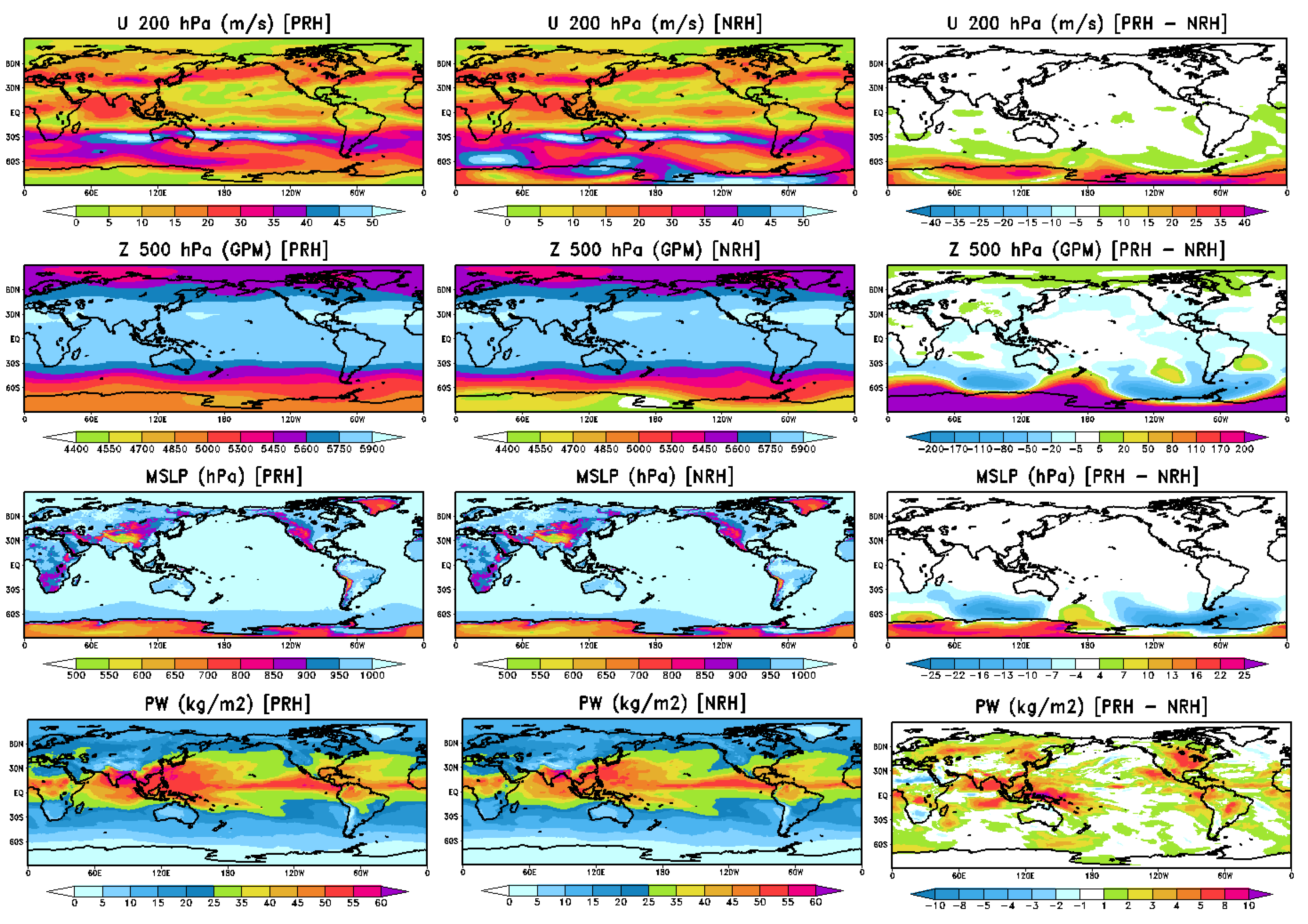
The sensibility of initial conditions for selecting moisture control variables in the assimilation was verified through the initial conditions of the mean fields of zonal wind at 200 hPa (U200 hPa), 500 hPa geopotential height (Z500 hPa), mean sea level pressure (MSLP), and precipitable water (PW). The mean fields were obtained to the experiments that utilized pseudo-RH, normalized RH and the difference between pseudo-RH and normalized RH in August (
Figure 1).
Greater differences were noted between normalized RH (NRH) and pseudo-RH (PRH) experiments in the Antarctic and region of the polar jet stream in the Southern Hemisphere when compared with the U200 hPa, Z500 hPa and MSLP fields (
Figure 1, right side). For the experiment utilizing PRH (
Figure 1, left side), the U200 hPa varied from 0 to 15 m/s, the Z500 hPa was 4700 m, and MSLP was between 600 hPa and 700 hPa at the Antarctic. In the region of polar jet stream in the Southern Hemisphere, U200 hPa ranged from 15 to 35 m/s, the Z500 hPa was 5450 m, and MSLP was 950 hPa. The U200 hPa results is consistent with the findings of a previous study [
20], which identified a zonal mean climatology wind of 10 m/s in 200 hPa at latitude of 80
S (Antarctic’s latitude) and a wind between 20 and 30 m/s at the region of polar jet stream.
The experiment using NRH (
Figure 1, center) achieved incoherent results with an average behavior of the atmosphere on the Antarctic and region of the polar jet stream in the Southern Hemisphere. This control experiment (NRH) showed similar rates to those presented in Cavalcanti et al. [
16]. The performance of Brazilian Global Model from CPTEC/INPE (without the coupling between GSI) was compared with a reanalysis of National Center for Atmospheric Research (NCAR-NCEP) by Cavalcanti et al. [
16] and revealed that the mean of U200 hPa is overestimated in 30
S and 60
S, achieving values between 30 and 40 m/s. These results are higher than rates obtained by reanalyzing NCEP-NCAR, i.e., between 25 and 35 m/s in austral winter (June, July and August).
Cavalcanti et al. [
16] observed the Southern Hemisphere at subtropical latitudes. They showed that the wavenumber 1 observed in the reanalysis of NCEP-NCAR is reproduced in the Brazilian Global Model model from CPTEC/INPE, but there are some differences in the intensity and position of zonal anomaly centers. The anomalous centers at mid- and high latitudes are weaker in the model than in the reanalysis, representing the weaker amplitude of the stationary wave in the model. Here, the PRH experiment was intenser than the NRH experiment in Z500 hPa.
The MSLP was underestimated in the Antarctic in the austral winter when evaluated with the reanalysis of NCEP-NCAR [
16]. Furthermore, the PRH experiment reached higher rates in comparison with the experiment using NRH (
Figure 1), i.e., PRH adjusts the bias identified in the NRH experiment. The data assimilation using the results obtained in the NRH experiment could not solve all the issues pointed out by Cavalcanti et al. [
16]. This is because the temperature observations on the Antarctic and region of the polar jet stream were not good enough to improve the fields. Nevertheless, the PRH experiment produced better results for these regions because they depend on the temperature forecast.
Cavalcanti et al. [
16] identified that the Brazilian Global Model presented a negative bias for temperatures between 1000 and 800 hPa in latitudes between 75
S and 90
S, as well as in levels over 700 hPa in latitudes around 60
S. An accurate result may be obtained if an appropriate monitoring system is installed on these locations. Nevertheless, Sapucci et al. [
21] demonstrated that AIRS-TPW was the only sensor to provide observations of air temperature on 15 June 2009. Therefore, the tools available in this study present a negative bias for air temperatures and a lack of observations. Dee et al. [
9] showed that the pseudo-relative humidity predicts relative humidity fairly well, depending on the accuracy of the background temperature estimates.
The precipitable water field produced the highest difference between the experiments. The highest variations were detected in several regions, such as the Kalahari Desert, the Northeast, Center and Northwest of South America, the Indian Ocean, West and East Pacific Oceans. The NRH experiment showed rates between 10 and 15 mm in the Kalahari Desert of Africa, while the PUR experiment showed rates between 15 and 20 mm (
Figure 1). Howarth [
22] found that this desert has one of the driest territories in the South Hemisphere. Therefore, the NRH experiment is consistent with Howarth [
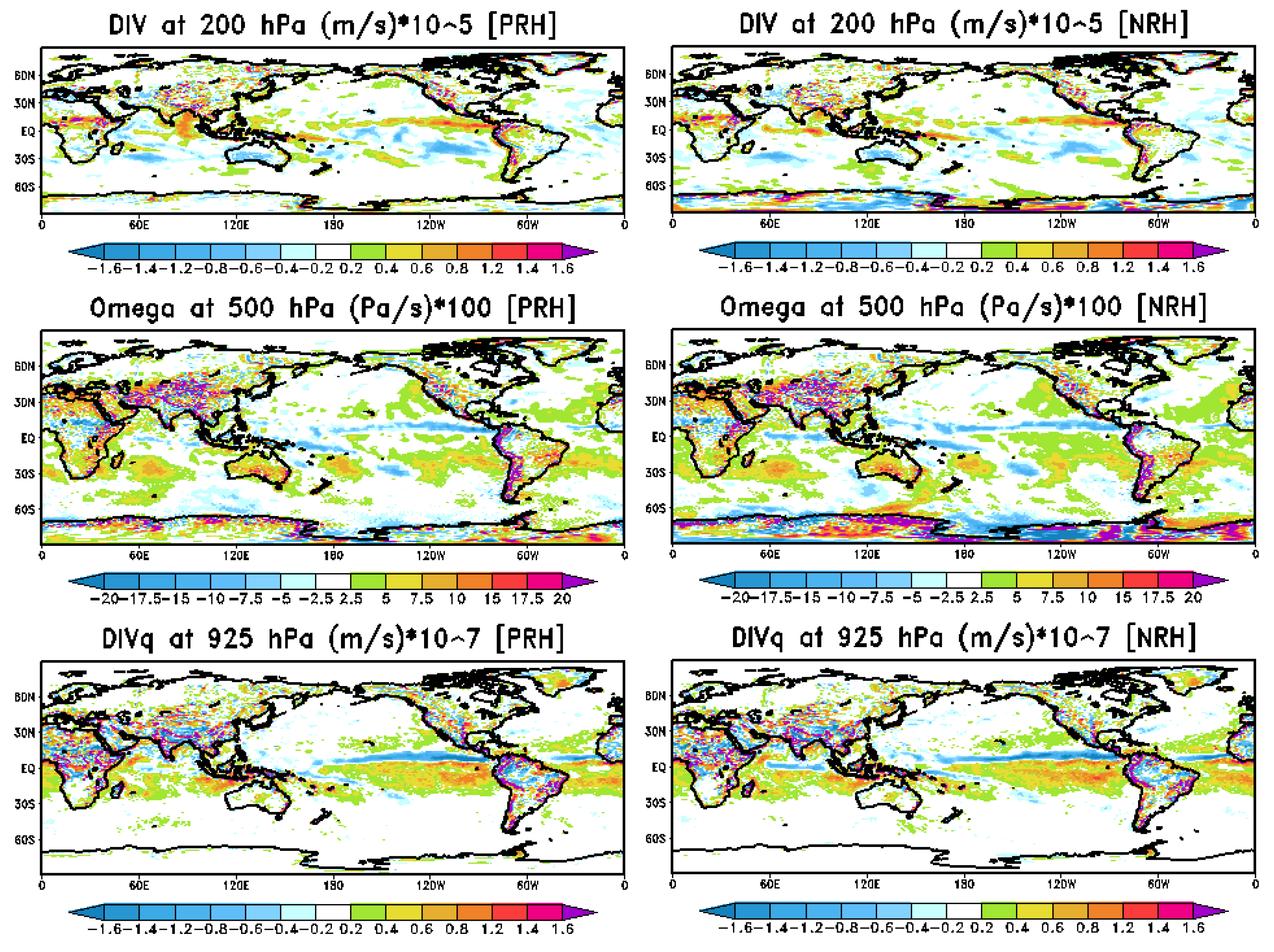
22]. This is because the experiment utilizing NRH indicated that the descending vertical movement in 500 hPA is slightly higher in the desert and more intensive over the southwest coast of Africa when contrasted with the experiment using PRH (
Figure 2).
In the tropics of the Indian Ocean, and the West and East Pacific Oceans, a divergence of mass, an ascendant vertical movement in 500 hPa, and humidity convergence flow was observed (
Figure 2). Altogether, these environmental variables make a proper analysis of rainfall. The PRH experiment showed minor intense values of these variables (
Figure 2). Howarth [
22] identified values of 50 mm of rainfall at tropics of the Indian Ocean and East Pacific Ocean, while the West Pacific was drier than the East Pacific. Howarth [
22] results were consistent with the RH experiment.
South America reached higher values of precipitable water on at northwest and center (
Figure 1). Rao et al. [
1] measured the rainfall in South America and found a higher volume at the Brazilian Northwest in July. The bigger difference between both experiments is over the center of South America because the humidity convergence at lower levels is stronger in the PRH experiment than in the NRH experiment.
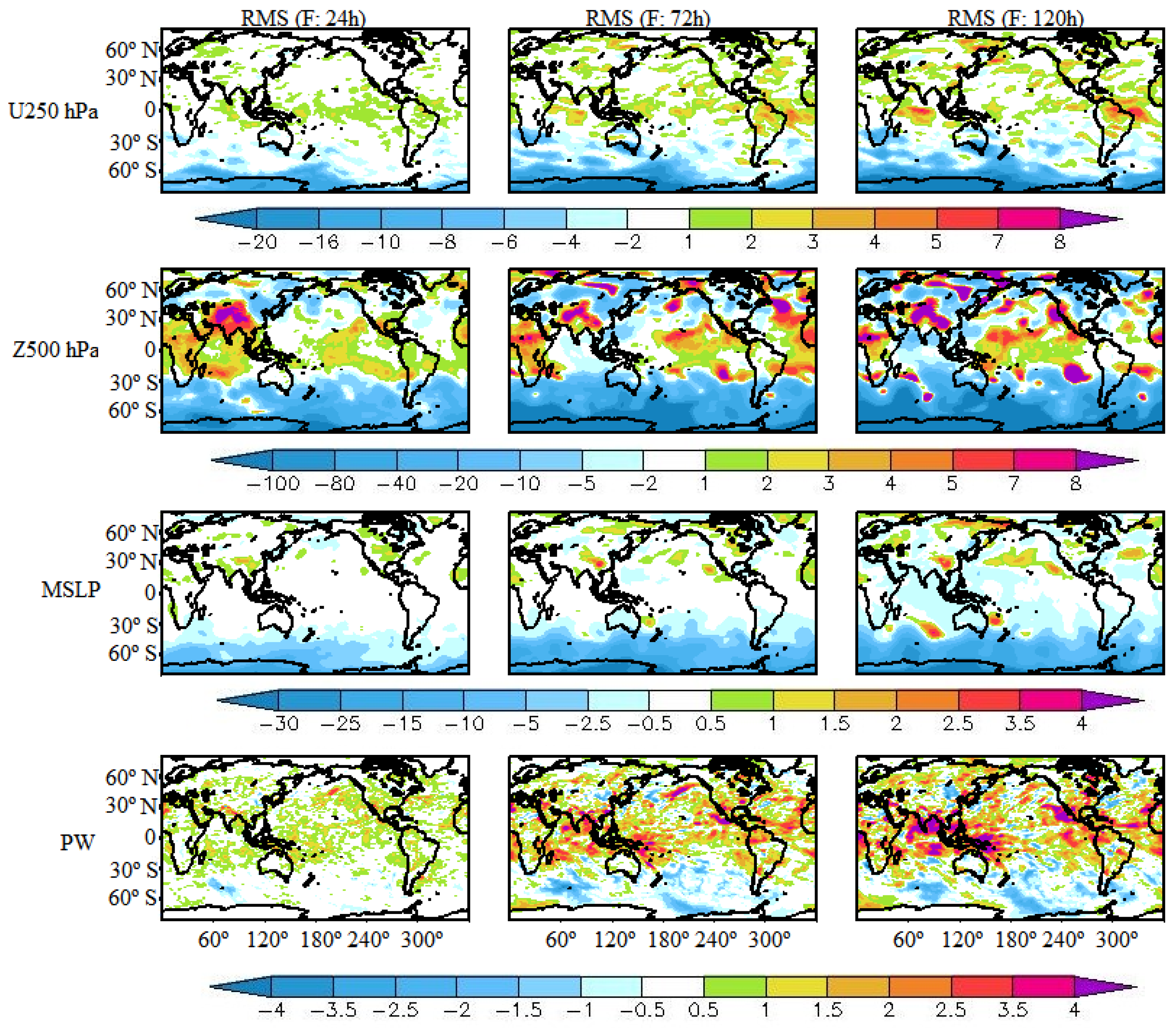
In a statistical analysis, differences in the root mean square (RMS) among the experiments have been evaluated. These experiments utilized the PRH and NRH variables in the forecasting of 24, 72, and 120 h to zonal wind fields at 250 hPa (U250 hPa), geopotential heights at 500 hPa (Z500 hPa), mean sea level pressure (MSLP), and precipitable water (PW) (
Figure 3). Then, positive values mean a greater difference between the 24, 72 and 120 h of forecast and the initial conditions to the PRH experiment, and negative values show a greater difference between the 24, 72 and 120 h of forecast and the initial conditions to the NRH experiment.
These results show that Brazilian Global Model tends to approximate the forecasts of 24, 72 and 120 h of the initial conditions in the fields of the basic state when PRH is used as a moisture control variable. There are subtle differences between the forecast and initial conditions in 30 S–90 S to MSLP and U250 hPa. These differences increase to Z500 hPa.
However, in the region of the polar jet stream in the Southern Hemisphere and in the Antarctic, greater differences are found for all variables of the basic state during the NRH experiment.
Figure 1 shows that the initial conditions of the fields of the basic state (U250 hPa, Z500 hPa, and MSLP) were more sensitive to experiment with PRH and
Figure 3 shows smaller RMS values in the forecasts of 24, 72 and 120 h over 30
S and 90
S region in this experiment. On the other hand, although the water precipitable fields were more sensitive over Kalahari Desert, South America and tropics, the Indian Ocean, and the West and East Pacific Oceans in the PRH experiment,
Figure 3 shows larger RMS values for the forecasts of 24, 72 and 120 h in these areas. This result indicates that Brazilian Global Model present deficiency in the suitable characterization of the humidity fields forecast considering the analyzed fields obtained when PRH is used as moisture control variable.
The sensibility of the initial conditions (
Figure 1) and of the forecasts (
Figure 3) in the choice of the moisture control variable is different over several parts of the globe. This difference is not constant along the evaluated period. To assess the temporal behavior of this difference,
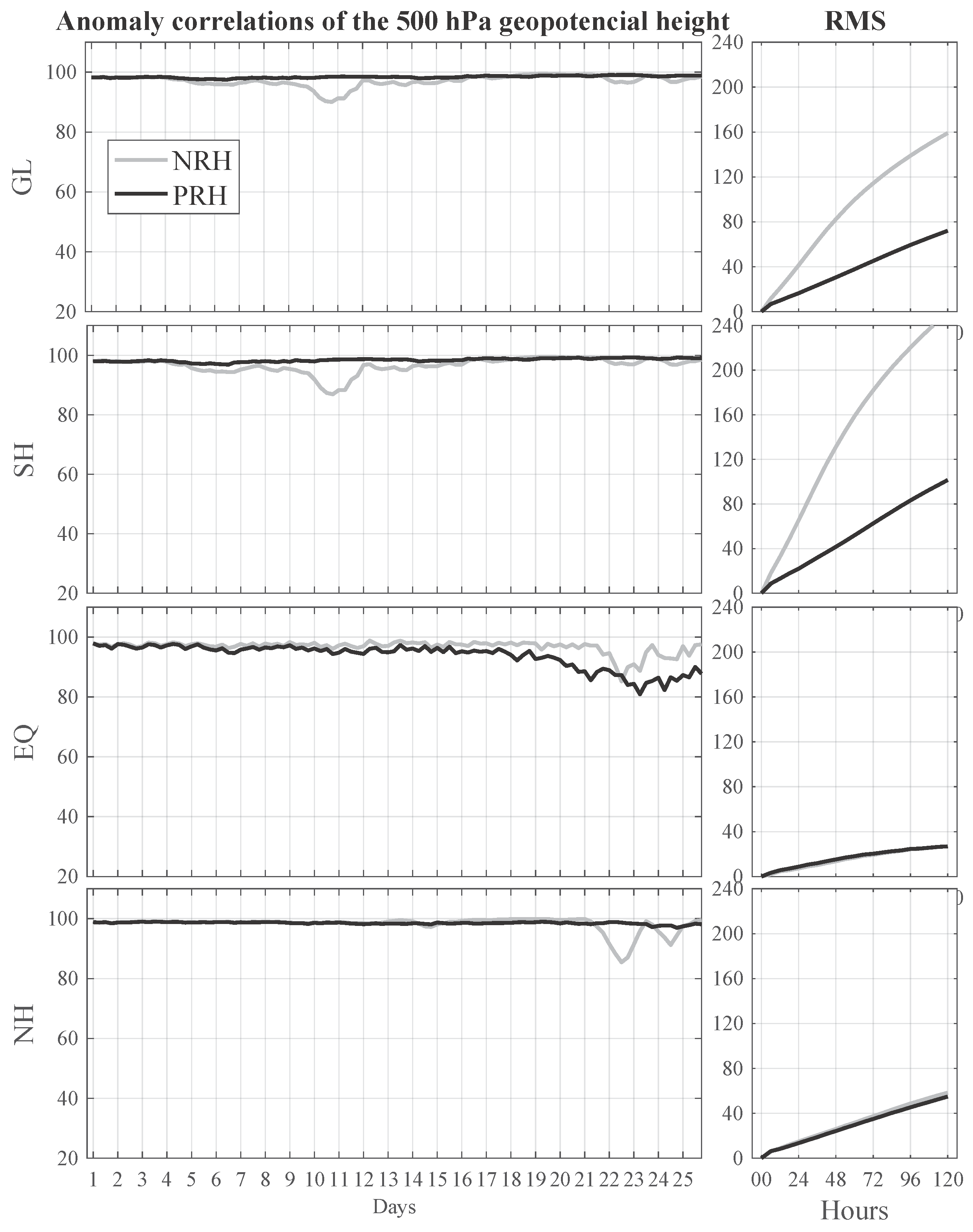
Figure 4 shows the temporal series of the anomaly correlation coefficient and RMS values of the forecast for 48 h with the height geopotential at 500 hPa as a function of the integration time for each experiment in the global domains, Southern Hemisphere, Equator and Northern Hemisphere in the analyzed period. This variable was chosen because it represents the basic state and has a relevant influence on the weather forecast in the extratropical areas, indicating the approach of frontal systems and high-pressure centers.
Figure 3 shows that there was little difference between the forecast and initial condition in the Southern Hemisphere during the PRH experiment and in the Equator during the NRH experiment. In
Figure 4, we can see the same behavior. The RMS value is lower for the PRH experiment than the NRH experiment associated with the Southern Hemisphere. The RMS value is equal between the PRH and NRH experiments over the Equator.
These results align with the analysis of
Figure 1, which showed that the PRH experiment is closer of the observed values in the reanalysis of NCEP-NCAR. On the other hand, the anomaly correlation values were degraded in the PRH experiment in Equatorial region, particularly after 20 days. In physical terms, the uncertainty is expected to be large where the atmosphere has a high capacity for water vapor, i.e., at low levels and high temperatures [
9].
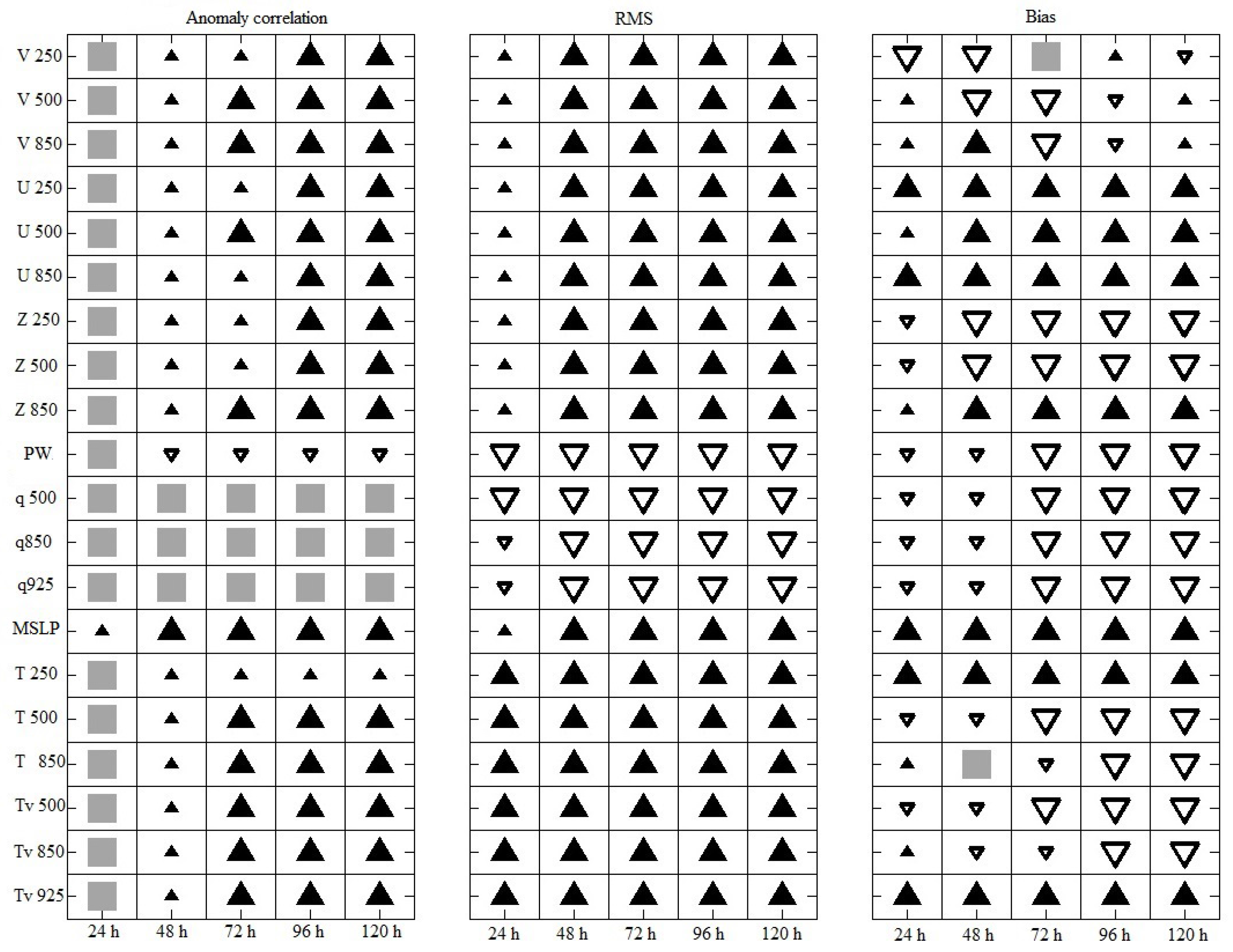
Figure 5 presents a summary of RMS, bias and anomaly correlation coefficient values among the initial conditions of 00:00, 06:00, 12:00 and 18:00 UTC and the forecasts of 24, 48, 72, 96 and 120 h of all the prognostic variables of the Brazilian Global Model. The variables are: zonal and meridional wind component (V and U); the geopotential height (Z) at 250, 500 and 850 hPa; water precipitable; specific humidity (q) at 500, 850 and 925 hPa; pressure at the mean sea level pressure (MSLP); air temperature (T); and virtual temperature (Tv) at 500, 850 and 925 hPa. The black triangles indicate that the PRH experiment was better than the NRH experiment and the inverted white triangle represents the opposite. The triangle sizes indicate the statistical significance of the metrics, small is less significant and the larger represents the opposite. The ash squares show that the values between the initial conditions and the forecasts are not statistically significant.
Figure 5 indicates the gain in the variable temperature dependence for the PRH experiment. This is represented as zonal and meridional wind components, geopotential height, the mean sea level pressure, the air temperature and virtual temperature. The basic state fields presented an anomaly correlation with statistical significance from 48 h of the forecast. The NRH experiment improved the humidity fields compared with PRH experiment, which presented smaller RMS values for water precipitation and specific humidity in all evaluated levels. The values of the anomaly correlation showed statistical significance from 48 h just in the field of the water precipitable. The bias values indicate that the NRH experiment generated a better forecast for the humidity fields. In this case, the forecast was systematically closer to the initial condition, and the results are better for larger model integration times.
In a synthesis of those results, the PRH should be a choice for moisture control variable when the model state needs to be maintained at a stable state during the assimilation cycle. However, this option punishes the forecast quality of the atmospheric humidity fields. On the other hand, when the data assimilation system is used to generate more appropriate humidity fields, the best choice is NRH. However, in that case, the basic state in the model is punished. In non-cyclical applications of the data assimilation and those that require high-quality precipitation forecasts, the NRH variable is the best option.
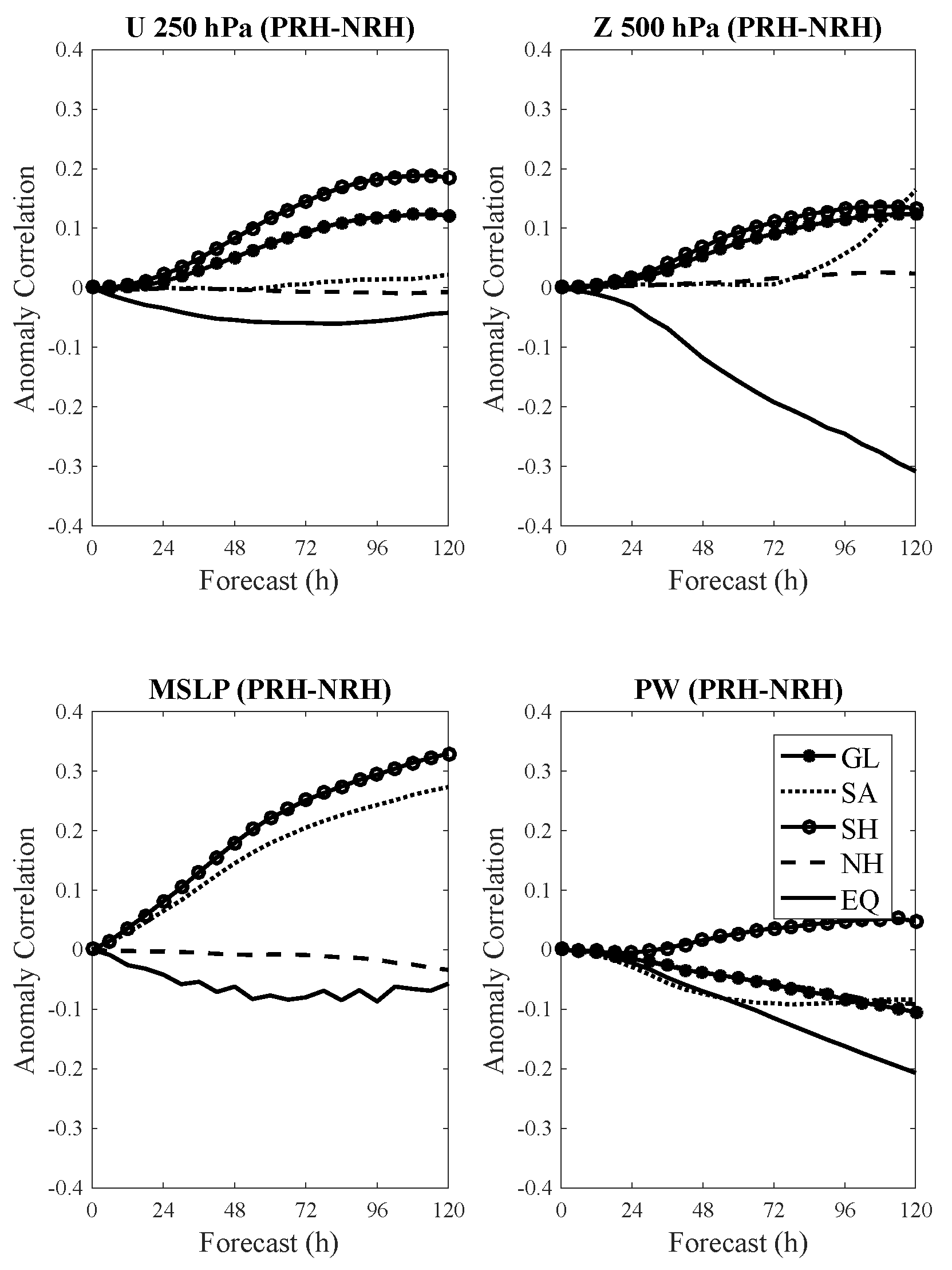
The previous results showed that the forecast fields generated by the model are distinct among different areas of the globe. This can be expressed as a function of the choice of the humidity variable control in the data assimilation system at CPTEC/INPE. To assess these results, a sensibility analysis of the forecast fields in different domains was carried out on differences of anomaly correlation coefficients obtained for PRH and NRH experiments.
Figure 6 shows the results as a function of the model integration time for the zonal wind component at 250 hPa, 500 hPa geopotential height, mean sea level pressure and water precipitable for the domains global, Southern Hemisphere, Northern Hemisphere, Equator region and South America. Note that positive difference indicates that the PRH experiment generated larger values of the anomaly correlation than the NRH experiment, and vice versa.
In
Figure 5, the PRH experiment presented better results than NRH experiment for the temperature-dependent variable of the global domain.
Figure 6 shows that domains such as the Southern Hemisphere and South America also presented superior values of anomaly correlation in the PRH experiment compared with the NRH experiment with the temperature-dependent variable (U250 hPa, Z500 hPa and MSLP).
The NRH experiment shows superior values of anomaly correlation over the Equator than the PRH experiment in PW, U250 hPa, Z500 hPa and MSLP. The biggest anomaly correlation for the NRH experiment was the Z500 hPa field at the Equator. In
Figure 4, the NRH experiment showed larger anomaly correlation after 20 August. The precipitable water was also a field with high anomaly correlation for the NRH experiment at the Equator. These results show that the choice of the NRH is the best option to use as a moisture control variable in the assimilation of data over the Tropical region.


