Abstract
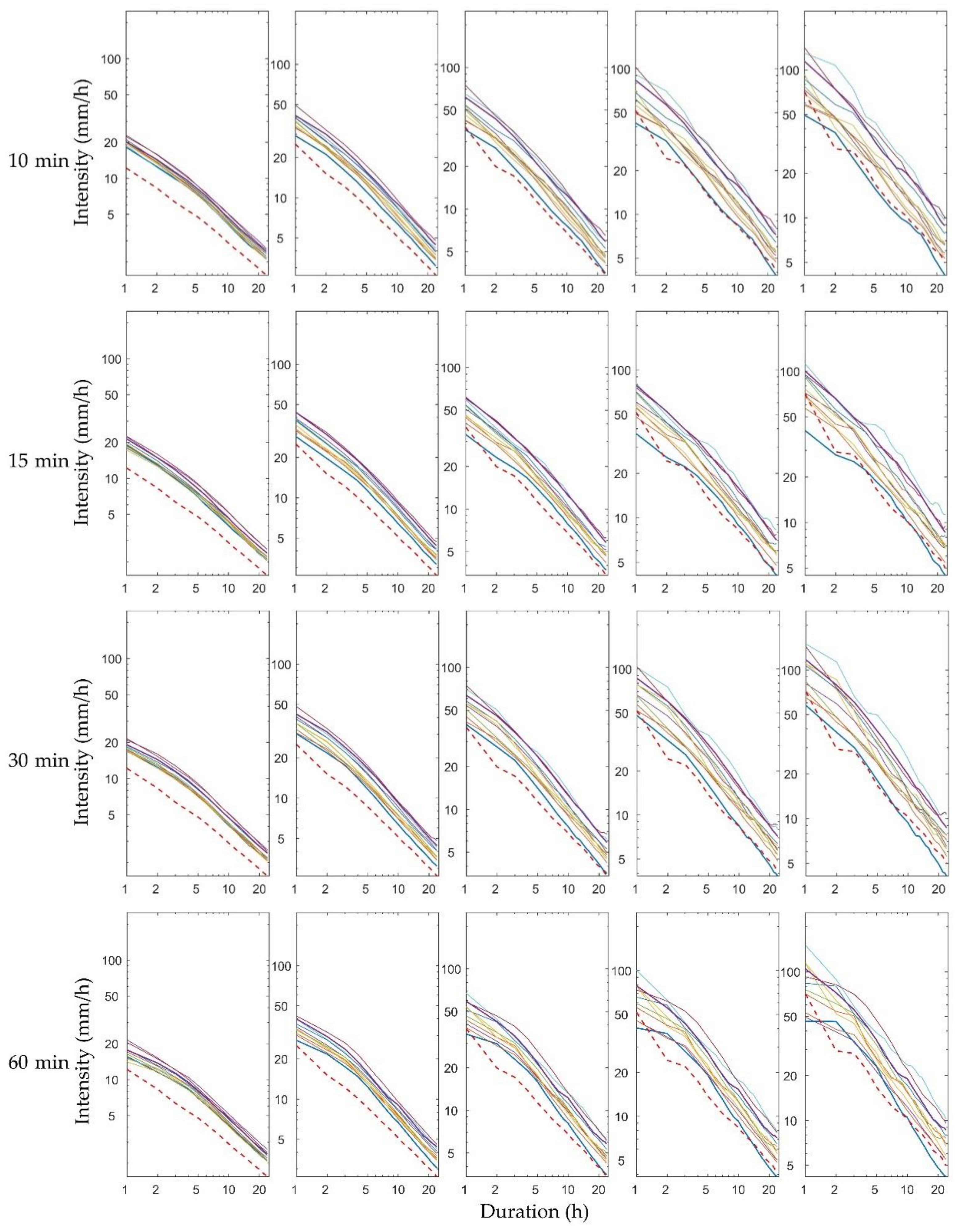
Designed for rainstorms and flooding, hydrosystems are largely based on local rainfall Intensity–Duration–Frequency (IDF) curves which include nonstationary components accounting for climate variability. IDF curves are commonly calculated using downscaling outputs from General Circulation Models (GCMs) or Regional Circulation Models (RCMs). However, the downscaling procedures used in most studies are based on one specific time scale (e.g., 1 h) and generally ignore scale-driven uncertainty. This study analyzes the uncertainties in IDF curves stemming from RCM downscaling ratios for four representative weather stations in the United Kingdom. We constructed a series of IDF curves using distribution-based scaling bias-correction technology and a statistical downscaling method to explore the scale-driven uncertainty of IDF curves. The results revealed considerable scale-induced uncertainty of IDF curves for short durations and long return periods; however, there was no clear correlation with the mean storm intensity of the IDF curves of different RCM ensemble members for each duration and return period. The scale-driven uncertainty of IDF curves, which may be propagated or enhanced through hydrometeorological applications, is critical and cannot be ignored in the hydrosystem design process; therefore, a multi-scale method to derive IDF curves must be developed.
1. Introduction
Large-scale climate change resulting from anthropogenic driving factors, such as excessive greenhouse gas emissions and urbanization, are modifying hydrological patterns in many regions worldwide. It is widely recognized that variations in the hydrologic cycle significantly affect the ecosystems and water circulation on which human social and economic life depends. In addition to enhanced climate variability, there is strong evidence that climate change is exacerbating the frequency and magnitude of extreme hydroclimatic phenomena, especially heavy precipitation events [1,2]. Therefore, studies of extreme hydrological events based on the nonstationary Extreme Value Theory in a changing environment are increasingly considered as necessary areas of research [1,3,4,5,6].
Intended to manage rainstorms and flooding, hydrosystems are generally designed using local rainfall Intensity–Duration–Frequency (IDF) curves. These curves, which characterize the durations and intensities of extreme precipitation events as they recur [7], are standard tools in storm water management systems, flood protection structures, and various other engineering designs involving hydrologic flows [8]. IDF curves are evaluated based on the assumption that the frequency, intensity, and return period of precipitation extremes are independent of any impact resulting from potential climate change [9]. However, rising concentrations of greenhouse gases in the atmosphere and rapid urbanization, which could shorten the heavy rainfall regression cycle, are making this assumption largely untenable. Therefore, the trends in IDF curves calculations are expected to move toward nonstationary or time-varying models to better respond to the changing environment and properly and precisely guide water management and hydraulic infrastructure design [1,10].
Given this background, appropriate methods are required to accurately update IDF and reduce uncertainties when accounting for anthropogenic changes in the atmospheric environment. There are two types of calculation models that can be used to evaluate variations in the intensity and duration of precipitation accounting for different recurrences and their uncertainties in a nonstationary climate. Regarding the first type, several studies have developed nonstationary approaches by modeling and analyzing trends in historically observed extreme rainfall series using covariates to build time-varying IDF curves [1,3,11]. Sarhadi and Soulis [3] proposed a nonstationary framework using a full time-varying generalized extreme value (GEV) distribution, in which temporal trends and the Southern Oscillation Index were covariates. In addition, Bayesian techniques have been used to examine the impacts of different and complex forms of nonstationarity on the extreme rainfall frequency in the Great Lakes area of the United States. Cheng and AghaKouchak [1] calculated time-dependent IDF curves by integrating a Bayesian-based Markov chain approach, which assumed the location parameter (μ) as a function of time, into the nonstationary GEV. Yilmaz [11] presented extreme value models using trend analysis and non-stationarity tests to detect potential influences of climate change on IDF curves in Melbourne, Australia. However, Agilan and Umamahesh [12] reported that applying time covariate-based linear trends directly in GEV or other distribution parameters may increase bias, with significant uncertainties related to the role of the covariates in the estimation of future rainfall IDF curves.
Apart from trend analysis methods, which develop IDF curves by modeling historical rainfall time series data, researchers have incorporated outputs from General Circulation Models (GCMs) or Regional Circulation Models (RCMs) using bias correction and downscaling to simulate non-stationary IDF curves [10,13,14]. Lehmann [10] integrated RCM outputs into spatial Bayesian hierarchical models to investigate the characteristics of future extreme rainfall events stemming from numerous climate change scenarios. Srivastav [14] updated the IDF curves using spatial and temporal downscaling, combining the changes in the distributional characteristics of the GCM/RCM between the baseline period and future period to assess the impact of climate change on future extreme precipitation. Lima [13] proposed a Bayesian beta distribution model to estimate IDF curves based on observed rainfall series and daily rainfall outputs under climate change scenarios provided by the GCM/RCM.
Although GCM/RCM output-based approaches can better reflect the physical basis than trend analysis methods, uncertainties are expected to result from the complicated processing steps as well as the amount and variety of data required. Therefore, the characterization, quantification, and reduction of the uncertainty of nonstationary IDF curves generated from GCM/RCM methods is necessary [15,16]. Two predominant uncertainties of statistical downscaling include uncertainty resulting from observed or GCM/RCM data (e.g., observation and measurement errors, choice of climate change scenario, or internal climate variability results from natural fluctuations) and uncertainty resulting from the technique or procedure adopted. Several studies have focused on uncertainties associated with insufficient quantity and quality of GCM/RCM or observation data [16,17]. For example, Willems et al. [16] used a Bayesian approach to quantify parameter uncertainty and uncertainties stemming from the use of multiple GCMs. Meanwhile, Nazemi et al. [17] found that the uncertainty of future IDF curves greatly influenced the choice of the shape parameters in the GEV model, particularly for large return periods.
Uncertainties caused by the adoption of specific techniques or procedures can be classified as bias-correction procedures and downscaling techniques. Bias-correction procedures are used to eliminate or remove systematic errors in GCM/RCM precipitation results based on observed precipitation data, whereas downscaling techniques aim to reduce the spatial and temporal coarseness of GCM/RCM simulation outputs. Kim et al. [18] demonstrated that some reasonable underlying distributional parametric uncertainty in RCM simulations could be corrected with a comparison test using bias-correction methods. Fadhel et al. [15] noted that the uncertainty in future IDF curves originated from the different reference periods used to correct the RCM precipitation bias, which have significant effects on future climate projections. Conversely, some studies have referred to the uncertainties associated with techniques involving spatial and temporal downscaling methodologies [16,17,18,19]. For example, Chen et al. [20] found a large uncertainty envelope related to the choice of using one of six distinct downscaling methods. In addition, Willems et al. [16] indicated that the uncertainty regarding the influence of downscaling on extreme precipitation data was high because the properties of extremes did not automatically reflect those of average rainfall.
Most studies have adopted a specific time scale for the temporal downscaling of future GCMs/RCMs. However, different time scales may lead to different downscaling results, and there has been little focus on the uncertainty associated with temporal downscaling ratios. If the uncertainty introduced by temporal downscaling is high, the nonstationary IDF curve calculated from the downscaled result will be unreliable since it uses only one type of time scale. This raises the following questions: Does temporal downscaling cause any uncertainty? If so, how much? What areas of the IDF curves reflect the impact of such uncertainties? To date, few studies have noted these issues; however, if this assumption holds, it is essential to determine a downscaling method based on a series of time scales to reduce uncertainty.
Therefore, this study aims to: (1) determine if uncertainties exists when different time scales are used to implement temporal downscaling and build a series of future IDF curves with the downscaled model results; (2) quantify the extent and source of any uncertainties by comparing a series of IDF curves; and (3) analyze the significance of the uncertainties stemming from RCM downscaling ratios.
2. Study Area and Data
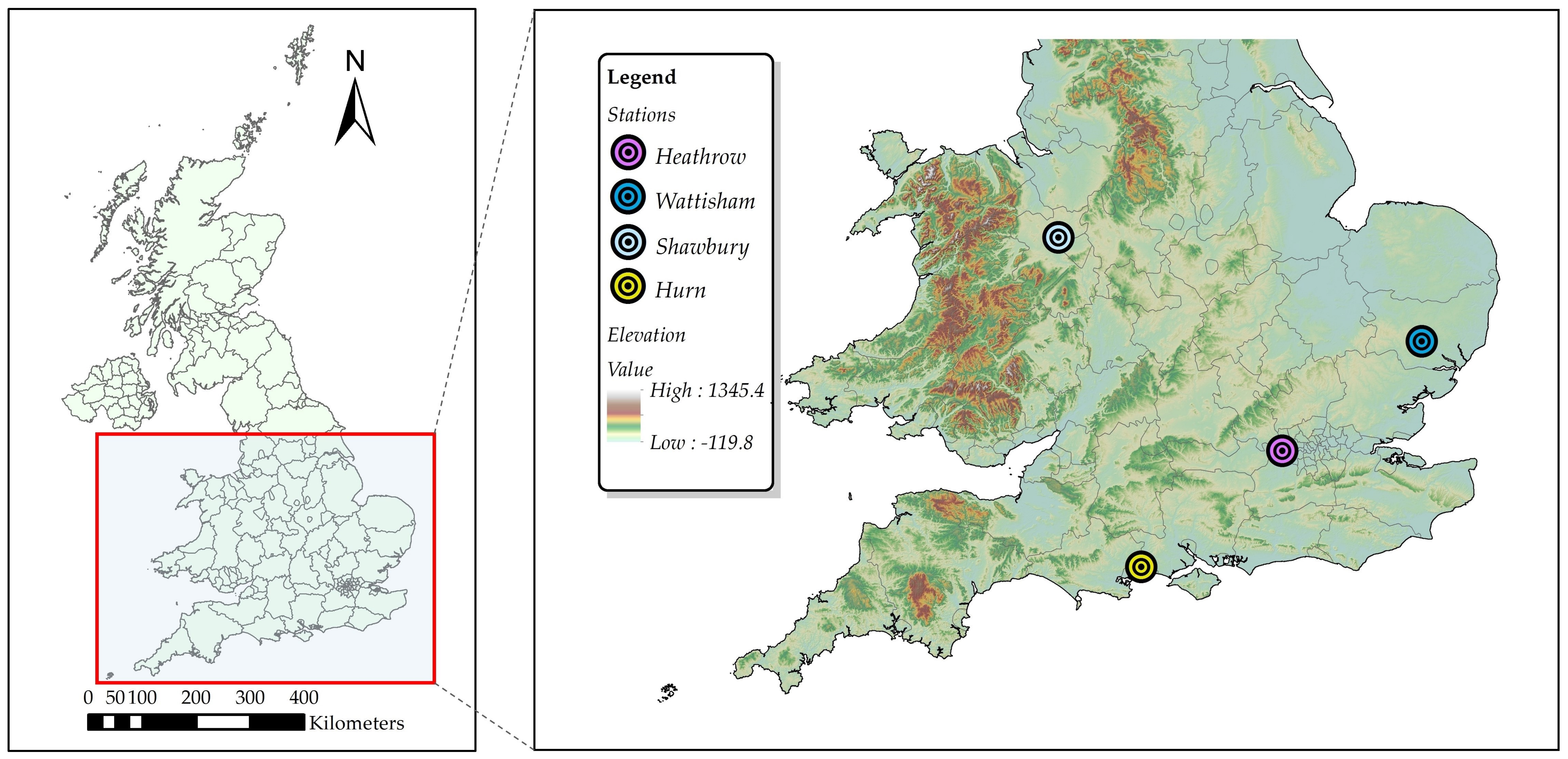
Heavy precipitation, which could lead to recurring flood events and cause serious damage to infrastructure, is of increasing concern in Europe [21]. Many studies have indicated an increase in the frequency and intensity of heavy rainfall in the United Kingdom (UK) [22,23]. The Met Office operates more than 200 automatic weather stations across the UK. In this study, we selected four representative weather stations in the south of England (Heathrow, Wattisham, Shawbury, and Hurn) with long period (more than 57 years) and high temporal resolution observation data to identify uncertainties stemming from RCM downscaling ratios in the IDF curves. The locations of the four selected stations are displayed in Figure 1, and Table 1 shows the mean and standard deviation of the annual maximum rainfall (mm) for five periods from 1960 to 2016.
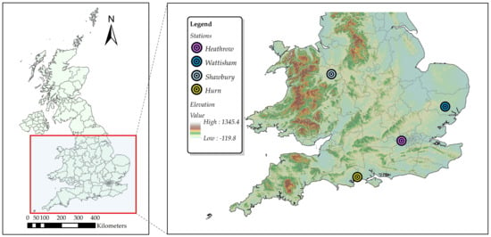
Figure 1.
Locations of the four study stations.

Table 1.
Mean and standard deviation (in parenthesis) of the annual maximum rainfall (mm) for five rainfall durations for the period of 1960–2016.
The datasets used in this study included historical observation data consisting of temperature, precipitation, the output temperature, precipitation data from an RCM, and radar data. Table 2 describes the purpose and time periods of the datasets.

Table 2.
Datasets used in this study.
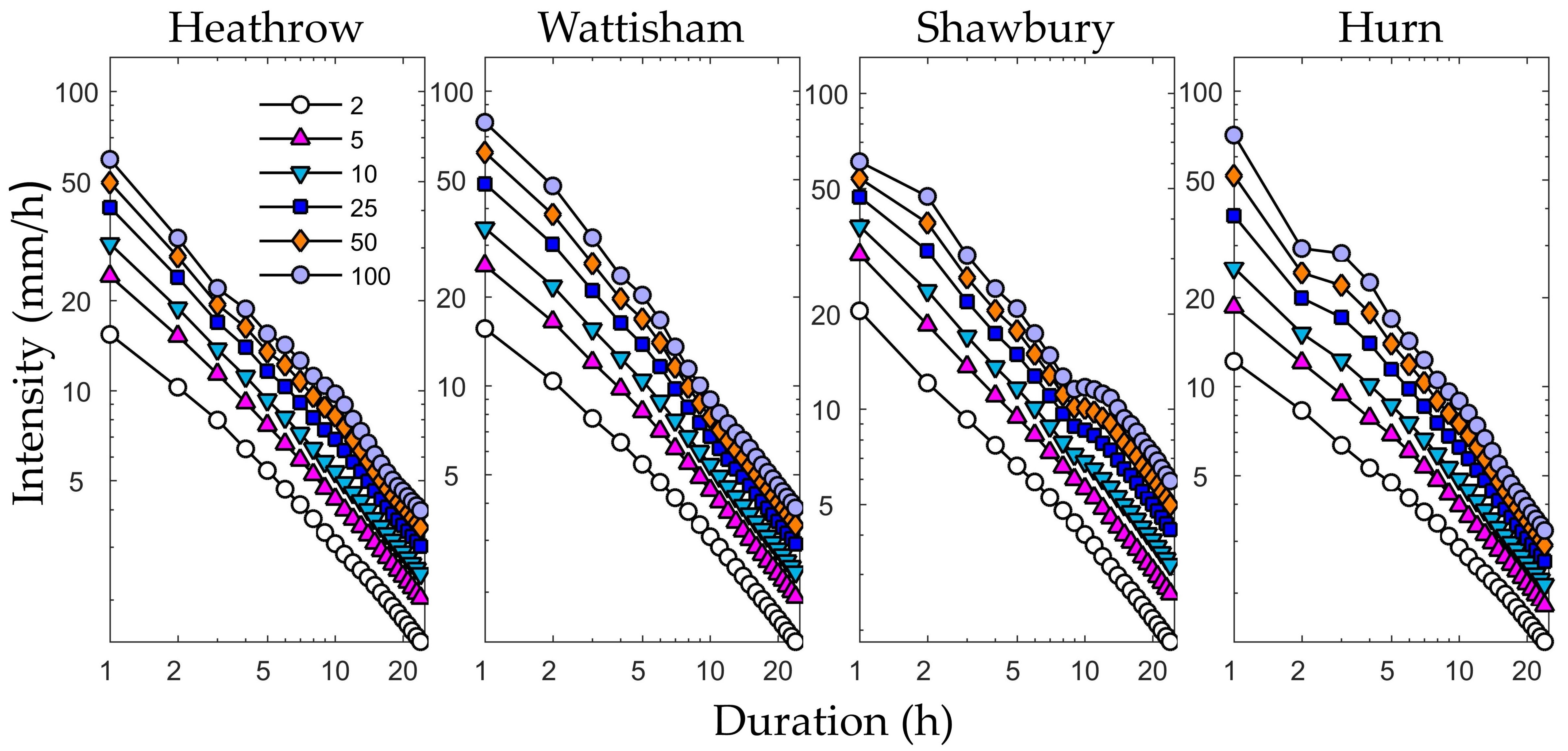
The observed temperature and precipitation data were obtained from the Met Office Integrated Data Archive System Land and Marine Surface Station Data [24,25]. To obtain historical IDF curves and correct the bias of daily precipitation data simulated by the RCM, we used long-term (1960–2016) hourly rainfall data from the UK. Figure 2 shows the historical IDF curves for return periods of 2, 5, 10, 25, 50, and 100 years [8,13] obtained from the annual maximum rainfall series (durations 1–24 h). There curves were generated with data from the four study stations fitted to the generalized extreme value (GEV) distribution suitable for modeling extreme rainfall [26] with the parameter locations (μ), scales (σ), and shapes (ξ) using the maximum likelihood estimation (MLE) method.
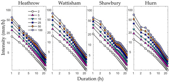
Figure 2.
Historical Intensity–Duration–Frequency curves for return periods of 2, 5, 10, 25, 50, and 100 years; the curves were obtained from the GEV (generalized extreme value) models fitted to the four stations’ maximum series.
To construct the future IDF curves, RCM datasets were obtained from the HadRM3 Perturbed Physics Experiment Dataset (HadRM3-PPE-UK) carried out by the Met Office Hadley Centre (Available online: http://catalogue.ceda.ac.uk) [27]. This dataset has a spatial resolution of 25 km, a daily temporal resolution, and offers time-series data from 1950 to 2100. The outputs of RCM were used to yield precipitations with sub-daily durations through downscaling methods. All 11 ensemble members of the RCM data for the periods 1960–2016 and 2040–2096 were the same length as the period of 1960–2016 used in this study. The RCM ensemble members were as follows: Q0 (HadRM3Q0), Q3 (HadRM3Q3), Q4 (HadRM3Q4), Q6 (HadRM3Q6), Q8 (HadRM3Q8), Q9 (HadRM3Q9), Q11 (HadRM3Q11), Q13 (HadRM3Q13), Q14 (HadRM3Q14), Q16 (HadRM3Q16), and Qk (HadRM3Qk). Each member was driven by the same historical and SRESA1B emissions, with one unperturbed member and ten members with different perturbations to the atmospheric parametrizations [27].
The radar data used to temporally downscale the RCM precipitation (from 24 h to 5, 10, 15, 30, and 60 min) spanning 2004–2017 were made available by the UK Met Office through the British Atmospheric Data Centre, with spatial and temporal resolutions of 1 km and 5 min, respectively. The residual errors in radar rainfall records have been computed for this case and were removed using observed rainfall records from the rain gauges [28,29].
3. Methodology
Owing to systematic errors present in the RCM, the original dataset cannot be used to calculate extreme future rainfall. Therefore, a bias-correction procedure based on observed data is essential to eliminate systematic errors (i.e., biases). In addition, the RCM rainfall scale (daily) must be disaggregated to a finer time scale (e.g., hourly) to construct IDF curves. However, most studies disaggregate the RCM scale to a specific scale without considering the uncertainties that this could introduce into the IDF. Therefore, in this study, RCM rainfall was downscaled from a daily scale to multiple hourly or sub-hourly scales to identify scale-driven uncertainties in the IDF curves. More specifically, RCM rainfall was disaggregated from a daily scale to 5, 10, 15, 30, and 60 min.
However, downscaling daily rainfall to different scales is complicated. The temporal resolution of the future rainfall data depends on the resolution of the historical rainfall. Although we obtained rainfall data at only two temporal resolutions (1 h for observed data and 5 min for radar data), the latter could be upscaled in multiples of 5 min and the future rainfall could be downscaled to different durations.
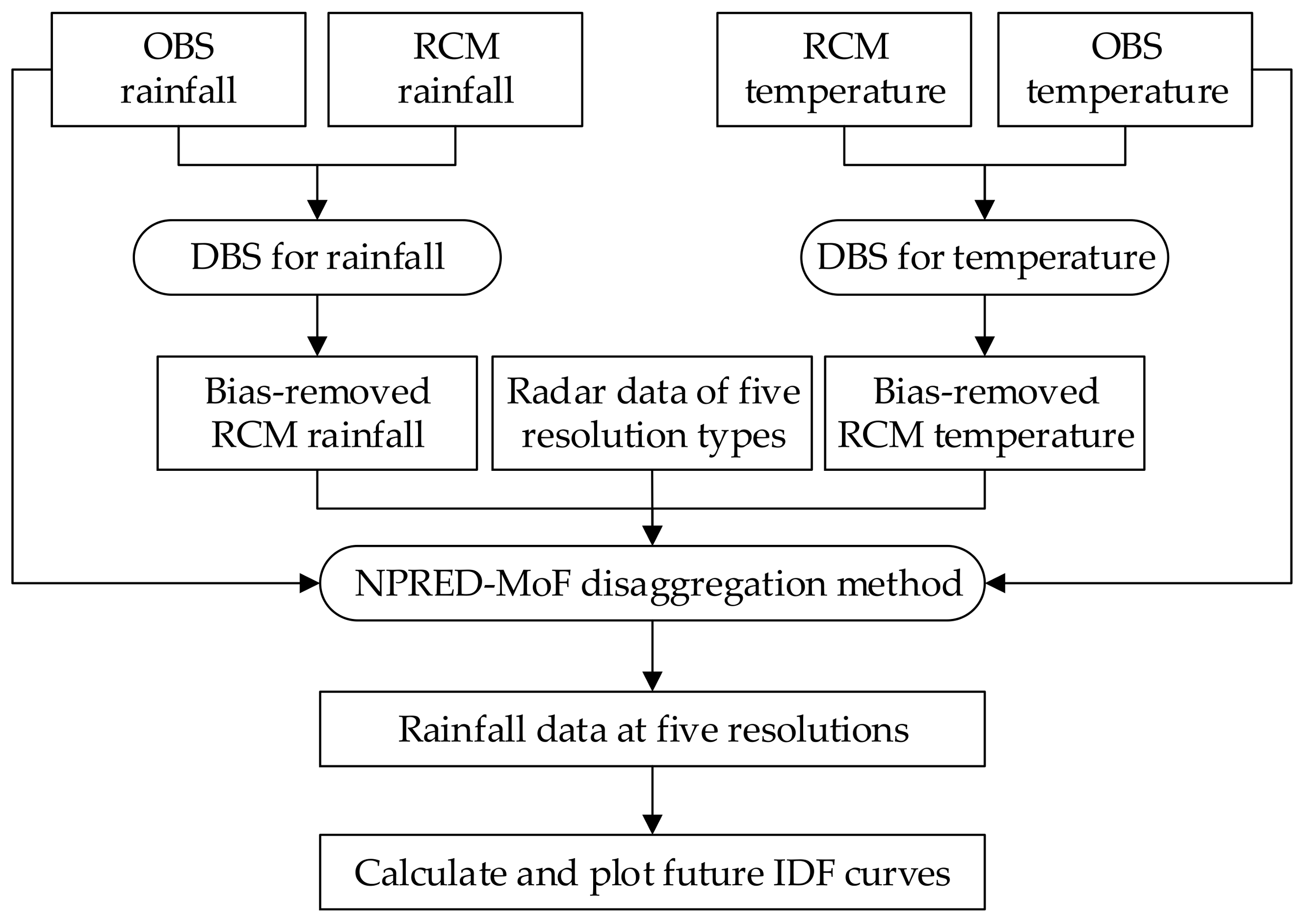
To further explore the scale-driven uncertainty of the IDF curves, future IDF curves from the four stations were constructed for five time scales and 11 RCM ensemble members using a distribution-based scaling (DBS) [30,31] approach to remove the bias of the RCM. A statistical downscaling method that combined nonparametric prediction models and the method of fragments framework (NPRED-MoF) [15] was used to disaggregate future daily rainfall to hourly or sub-hourly scales. The construction procedure of the IDF curves for each RCM ensemble member and each station is presented in Figure 3. First, we applied the bias correction for RCM precipitation and temperature based on the DBS approach. The input dataset was the historical observed and RCM rainfall and temperature, and the output dataset was bias-removed RCM rainfall and temperature. Second, we disaggregated the future rainfall from a daily resolution to five temporal resolution durations based on the NPRED-MoF method. The input dataset was the bias-removed RCM rainfall and temperature, radar data, and historical observed rainfall and temperature, and the output dataset was the future rainfall data of the five hourly and sub-hourly resolutions. Finally, the annual maximum rainfall for 24 durations of 1–24 h were extracted and fit to the GEV distribution to identify the maxima using the MLE method. The rainfall intensities for different return periods (2, 5, 10, 25, 50, and 100 years) were then calculated, and the five types of IDF curves based on the rainfall intensity from six return periods and 24 durations could be plotted.
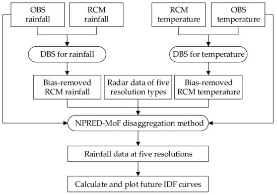
Figure 3.
Procedure used to construct the future IDF curves.
In this study, the bias-correction procedure for the RCM precipitation and temperature predominantly depended on the DBS approach described by Yang et al. [30] and Olsson et al. [31]. This method adjusts the distribution of RCM data to make it consistent with the distributions of the observation data based on cumulative distribution functions (CDFs) and then determines the new RCM data distribution parameters estimated by the maximum likelihood.
A temperature based on a Gaussian distribution [30] is more consistent with the parameters of the mean (μ) and standard deviation (σ). Therefore, the DBS approach to correct biases in temperature depends on a Gaussian distribution. The DBS procedure for temperature was implemented using a 15-day moving window to obtain parameters [30] without separating the wet days [31].
A gamma distribution has been found to be effective in determining the distributions of precipitation events using the shape (α) and scale (β) parameters [32,33]. We used a double-gamma distribution which divided the observed and RCM data into two parts based on the 95th percentile of the CDF to remove biases in the RCM precipitation data, to better capture extreme precipitation events and calculate the parameters based on a monthly segment [31].
We used a NPRED-MoF framework statistical downscaling method, as in Fadhel et al. [15], for the disaggregation process. The NPRED model was applied to predict the maximum storm burst fractions at the same duration as the downscaled future daily rainfall to be disaggregated using daily rainfall and temperature predictors. The experiments to predict storm burst fractions were based on open-source NPRED software for R [34], which uses partial information correlation (PIC) logic to detect predictors and partial weights (PW) to predict the response [34,35]. The NPRED tool was used without separating the data into seasonal segments for more precise predictions, as suggested by Fadhel et al. [15].
On the basis of results predicted by the NPRED model, the MoF framework developed by Mehrotra et al. [36] and Westra et al. [37] was adopted to disaggregate future daily rainfall into hourly or sub-hourly fragments or sequences. This framework resamples the sub-daily rainfall fragments from the historical rainfall series by determining the historical days with atmospheric conditions “similar” to future climates. Further details can be found in Mehrotra et al. [36] and Westra et al. [37].
We disaggregated future daily rainfall into five hourly and sub-hourly fragments using the same the disaggregation steps for each fragment. The disaggregation procedure, based on the NPRED tool and MoF framework for each duration, consisted of two principal steps for each fragment. The first step was to predict the future storm burst fraction based on the NPRED tool and to calculate the historical fractions found when the maximum storm burst rainfall was divided by the total rainfall of each day based on radar data with a 5 min resolution. The second was to construct a model for two predictors (historical temperature and rainfall) using the historical fractions as the response variables; the constructed model was then applied to the future climate to determine future fractions using future temperature and rainfall as predictors. An additional step included obtaining the full hourly or sub-hourly temporal pattern of the future climate based on results from the first main step and the MoF framework. For each future day, we used the MoF framework with a 15-day moving window [38] to find days with an atmospheric state “similar” to the daily rainfall resolution day in the future. We then applied the rainfall pattern of one of the identified days to the future day [37].
4. Results and Discussion
4.1. IDF Curves for Future Climate
We applied the DBS approach to correct biases and adopted the NPRED-MoF method to temporally downscale the RCM. To explore the uncertainties present in the IDF curves due to the RCM downscaling ratios used, we disaggregated the future modeled rainfall data into five hourly or sub-hourly durations. A series of future IDF curves was estimated for the examined weather stations based on the five time scales to determine how these temporal resolutions impacted future climate IDF curves.
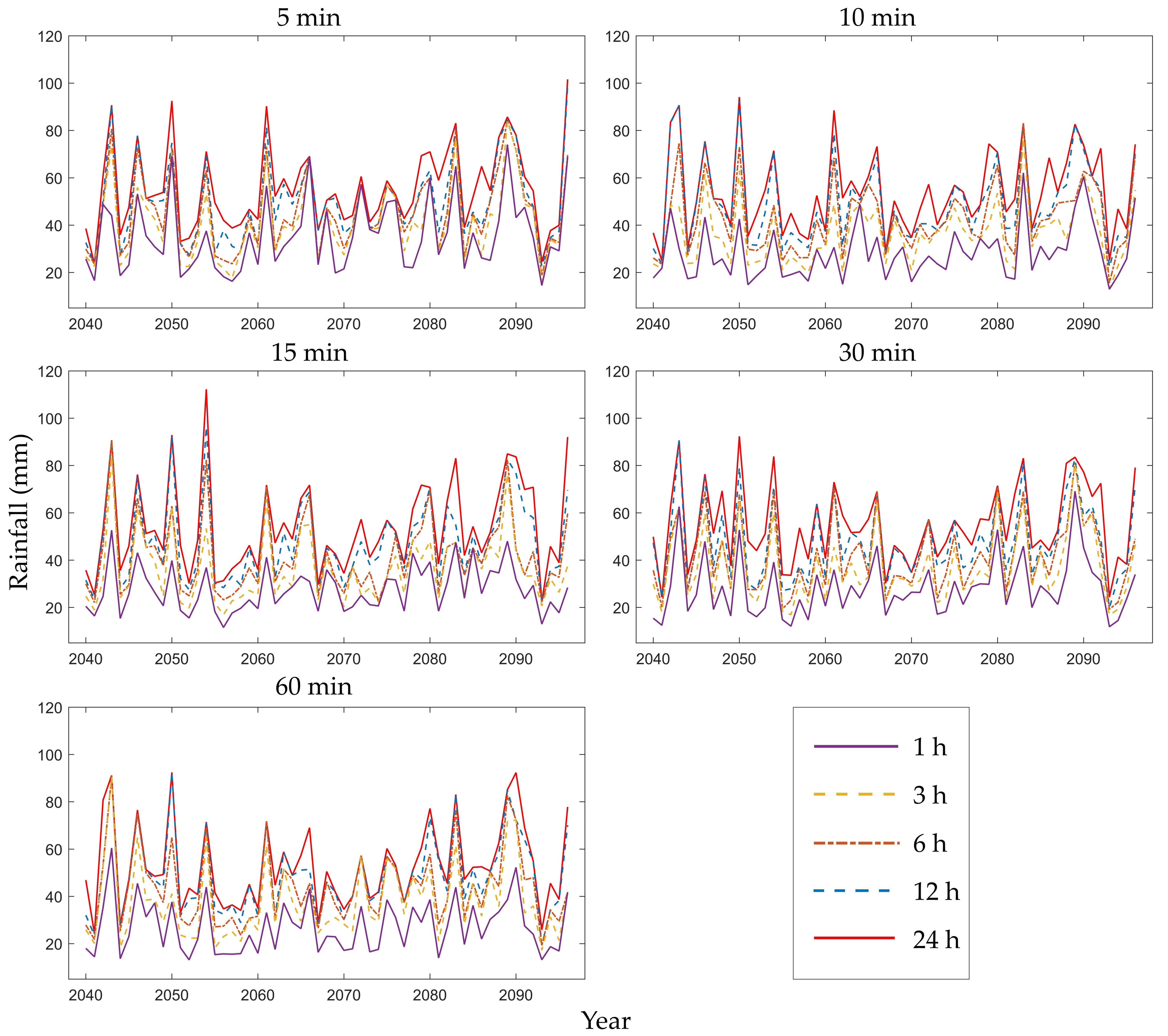
Figure 4 displays the annual maximum rainfall series for the period 2040–2096 at the Heathrow station for 1, 3, 6, 12, and 24 h; the results were based on temporal resolutions of 5, 10, 15, 30, and 60 min for the first RCM ensemble member (Q0). The overall distributions were similar to those of the five time scales, but the local differences were significant, implying that the IDF curves may have been dissimilar.
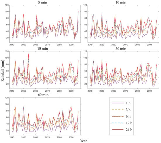
Figure 4.
Future annual maximum rainfall series of different durations (1, 3, 6, 12, and 24 h) based on different RCM downscaling ratios (5, 10, 15, 30, and 60 min) for Heathrow station and the first RCM ensemble member (Q0).
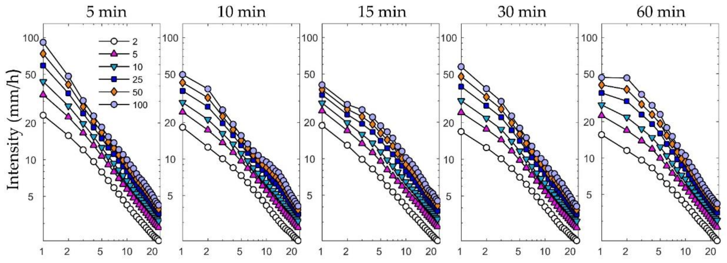
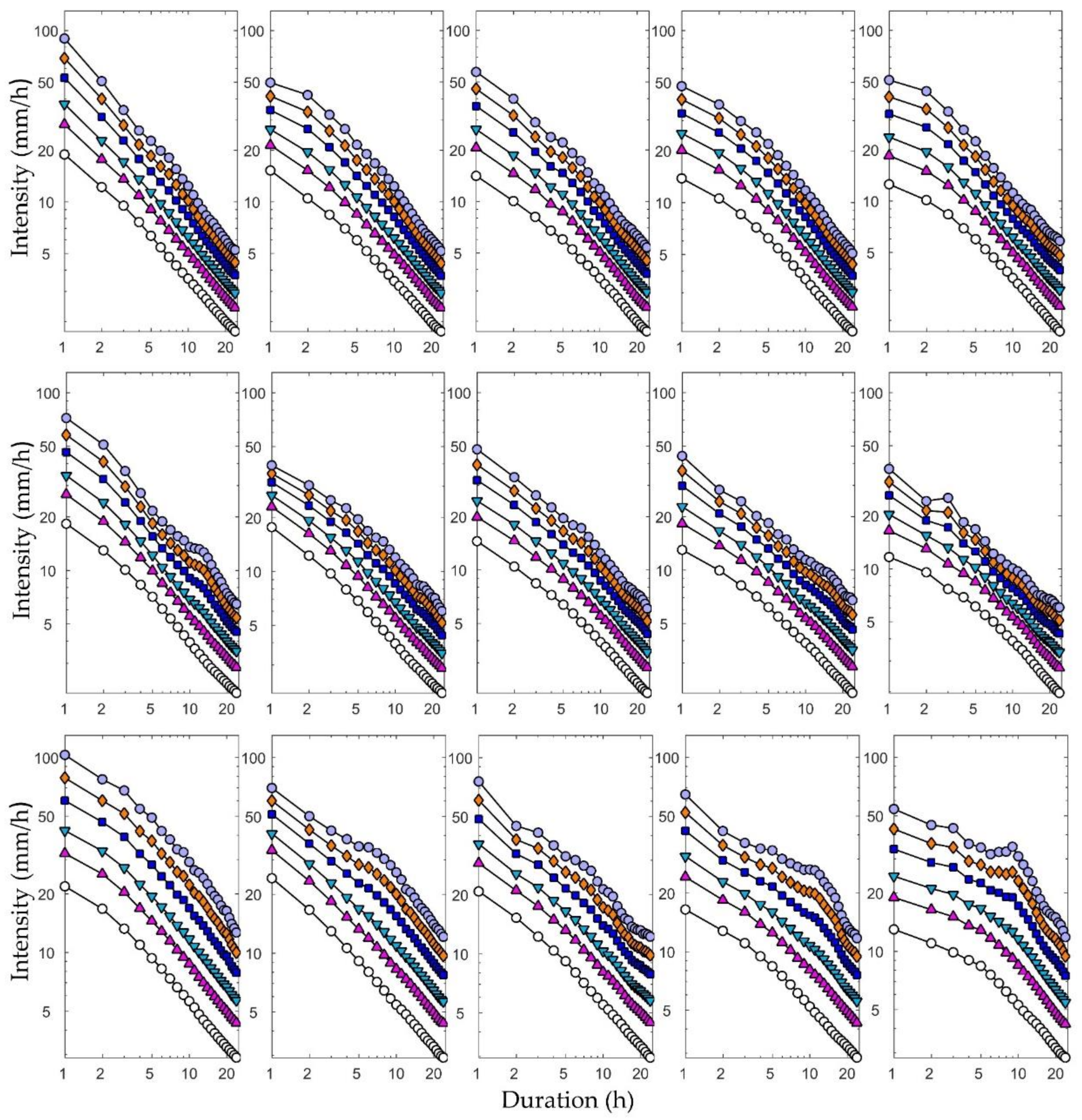
Moreover, we obtained the future rainfall distribution for 24 durations of 1–24 h by fitting the modeled extreme rainfall data to a GEV distribution. The future IDF curves could then be developed by estimating the empirical quantile associated with the six chosen return periods and dividing it by the given durations. The future climate IDF curves obtained for the first ensemble member from Heathrow, Wattisham, Shawbury, and Hurn (top to bottom) are displayed in Figure 5. Each subplot, the six return periods, and the 24 rainfall durations were based on one specific time scale. Unsurprisingly, there were clear differences in the IDF curves corresponding to the five temporal resolutions, especially for the shorter durations, at each station. Interestingly, rainfall appeared to be more intense at the 5-min temporal resolution than at the other resolutions for short durations.
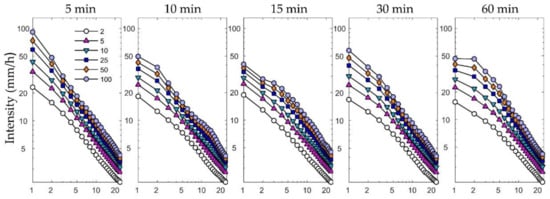
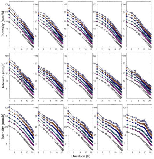
Figure 5.
Future IDF curves for (from top to bottom) Heathrow, Wattisham, Shawbury, and Hurn stations, for return periods of 2, 5, 10, 25, 50, and 100 years, obtained from GEV models based on five RCM downscaling ratios for future rainfall maxima.
4.2. Uncertainty of IDF Curves Due to Downscaling Ratios
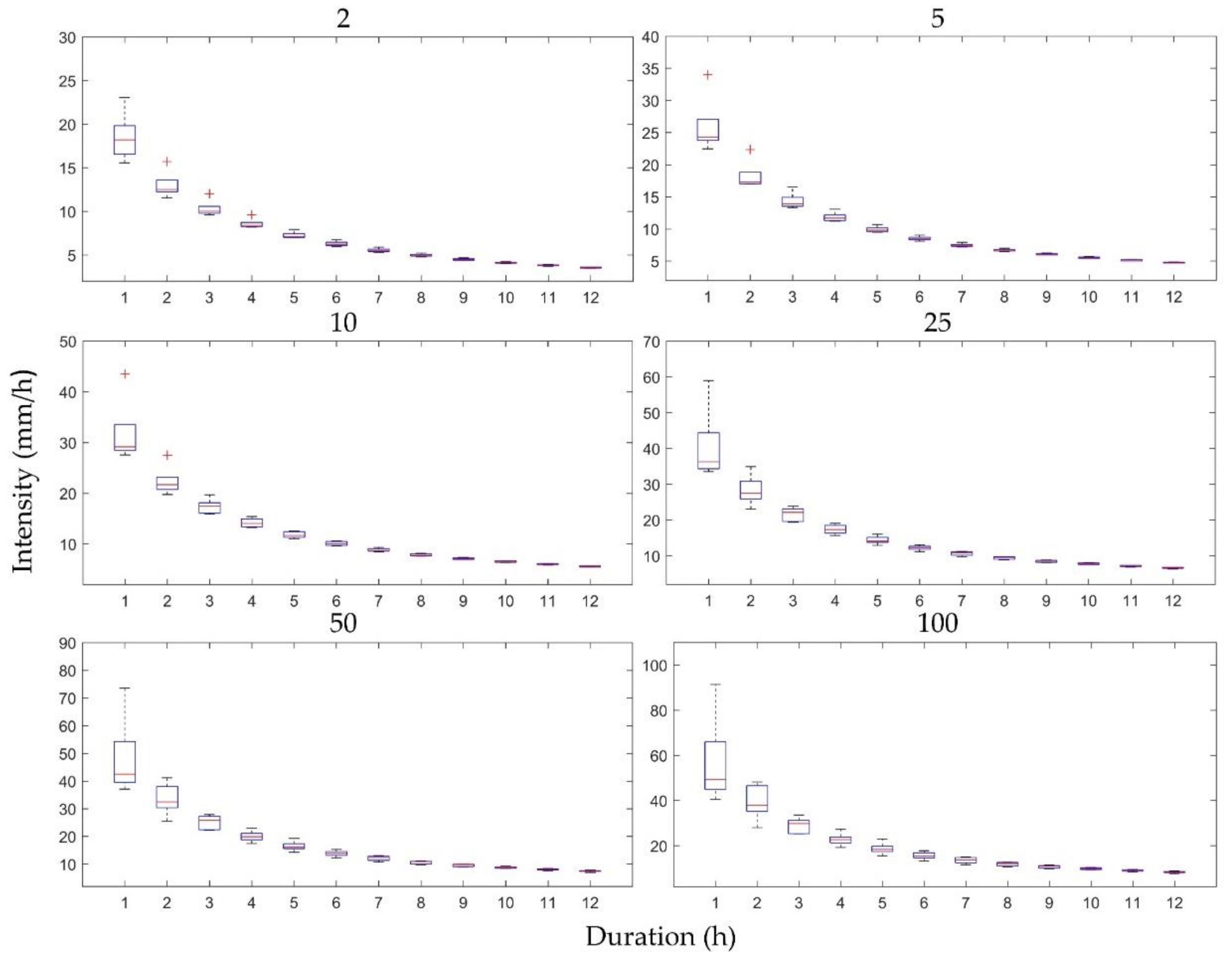
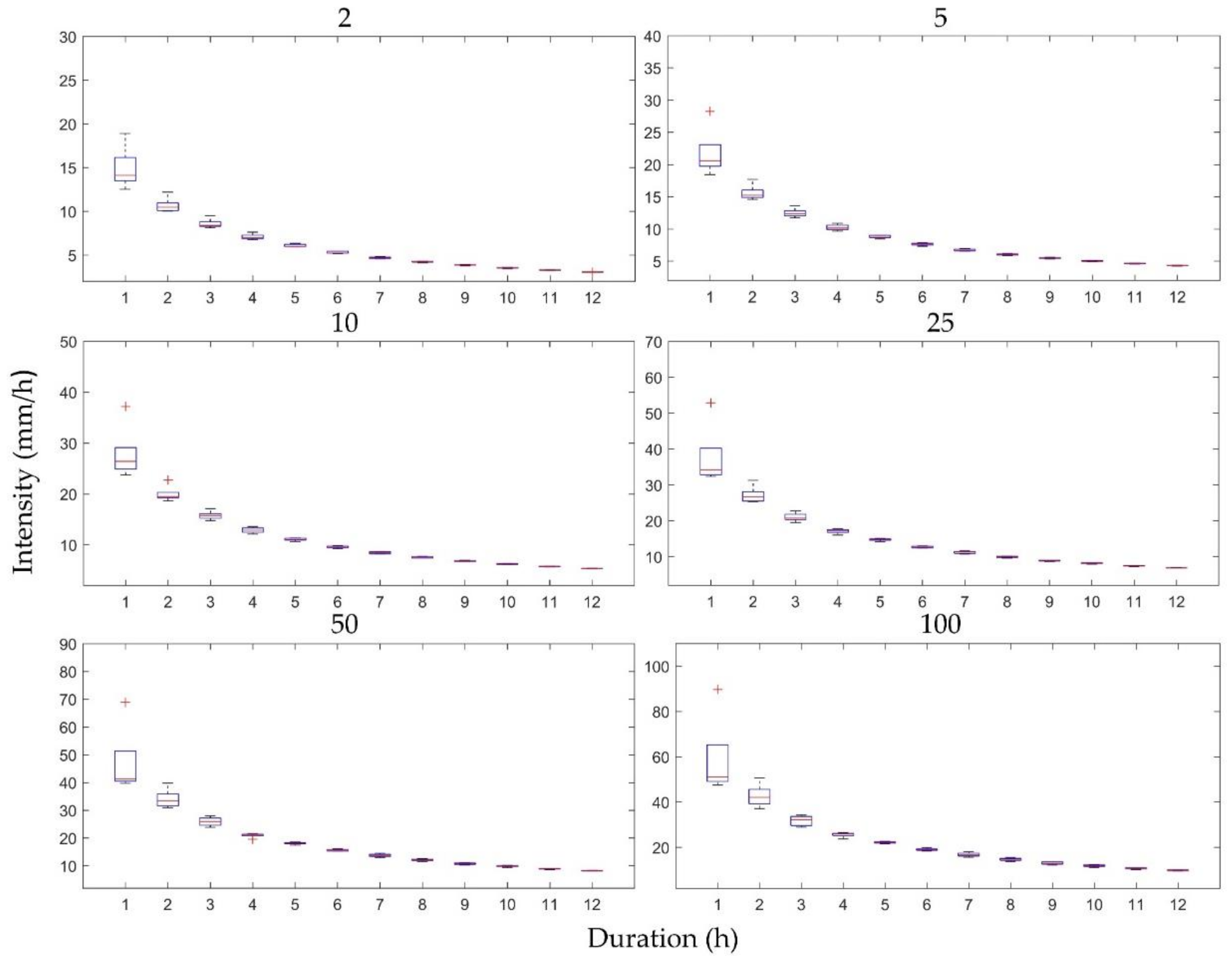
The uncertainties of the future IDF curves resulting from downscaling RCM ratios were characterized as box plots of the IDF curves based on the five temporal resolutions and the first RCM ensemble member for the six return periods (2, 5, 10, 25, 50, and 100 years) for Heathrow (Figure 6) and Wattisham (Figure 7) stations. These plots show the differences only for 12 durations (1–12 h), because the differences between the other durations were too small to observe in box plots. Notably, the differences in the IDF curves in Figure 6 and Figure 7 were considerably higher for shorter durations and seemed to follow a downward trend as the durations lengthened. Shawbury and Hurn stations showed similar trends.
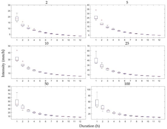
Figure 6.
Differences in the IDF curves of future rainfall resulting from five downscaling ratios for Heathrow station. Each subplot represents a specific return period and for 12 rainfall durations.

Figure 7.
Differences in the IDF curves of future rainfall resulting from five downscaling ratios for Wattisham station. Each subplot represents a specific return period and for 12 rainfall durations.
For further quantitative analysis, the mean, standard deviation (SD), and coefficient of variation (C.V.) of the rainfall intensity of the five time scales are presented in Table 3 and Table 4. The mean and SD for Heathrow and Wattisham stations decreased as the duration for each return period increased, and increased with each increasing return period for most of the durations. The C.V. appeared to follow the same trend, with several exceptions (e.g., the C.V. at 24 h was greater than that at 12 h for Wattisham station).

Table 3.
The mean, standard deviation (SD), and coefficient of variation (C.V.) of rainfall intensity for five time scales, three return periods, and five durations for the data from Heathrow station.

Table 4.
The mean, standard deviation (SD), and coefficient of variation (C.V.) of rainfall intensity for five time scales, three return periods, and five durations for the data from Wattisham station.
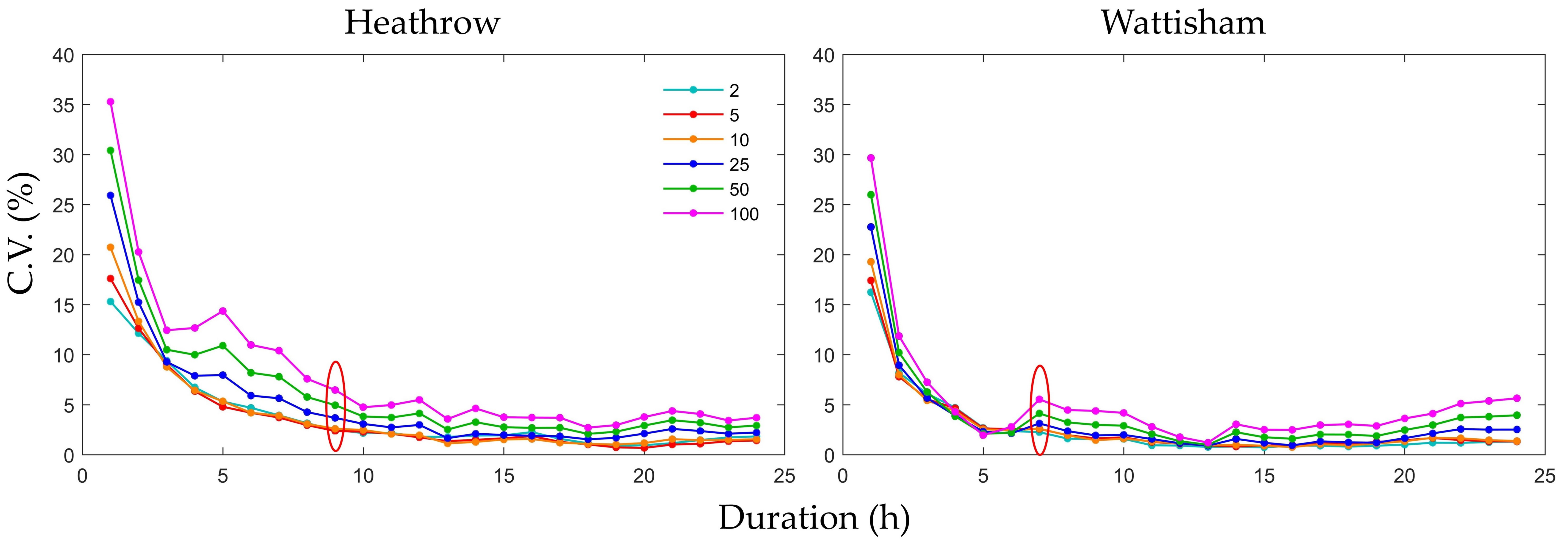
The C.V. distributions for the same durations, return periods, and stations were plotted (Figure 8) to determine the relationship between the C.V. and the durations of different return periods. The C.V. decreased exponentially with increasing durations for each return period and increased as with each increasing return period for each duration. Both stations exhibited turning points, after which the C.V. did not decrease with increasing duration (at 9 h for Heathrow station and at 7 h for Wattisham station), and the C.V. was below 5% in most cases after those points. These results imply that the influence of the downscaling ratios on the uncertainties of the curves are significant below a certain duration (generally between 5 and 10 h) at each station. In other words, the uncertainty associated with scale can be ignored when the duration is higher than the turning point. Moreover, the increasing trend as a return period lengthens is more conspicuous for shorter durations (1 or 2 h).
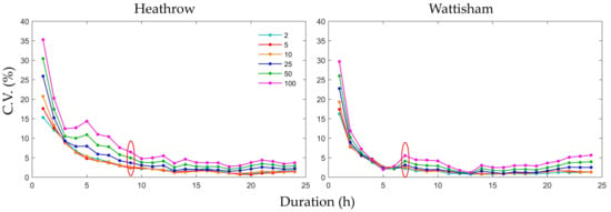
Figure 8.
Coefficient of variation (C.V.) distributions of the rainfall intensity of the five types of IDF curves based on five downscaling ratios for six return periods and 24 durations for Heathrow and Wattisham stations. The dots in red ellipses are turning points.
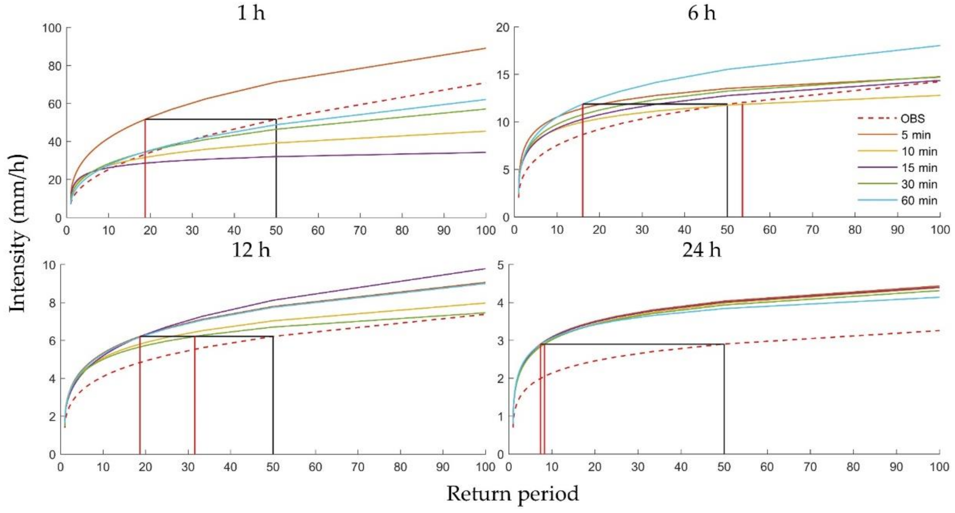
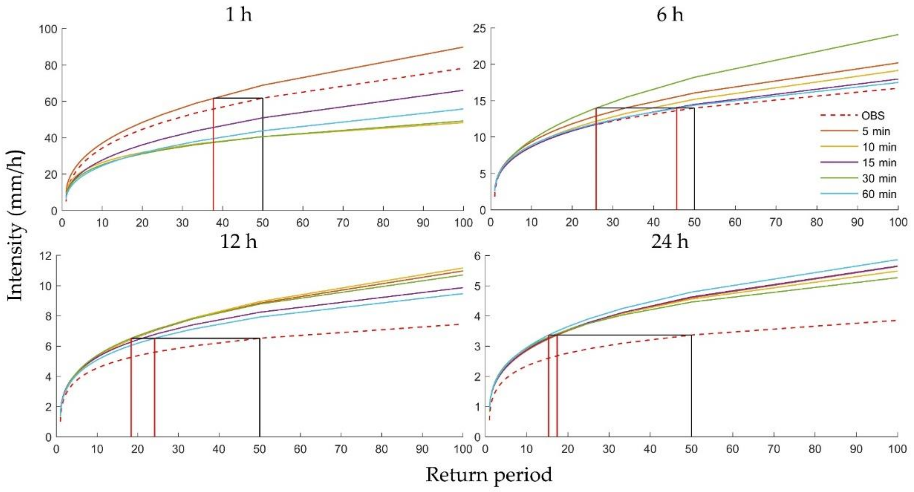
To further explain the relationships between the uncertainties and the historical climate, rainfall duration, and return period, Figure 9 and Figure 10 show the rainfall intensity of the historical and future climate predicted with five downscaling scales for four durations (1, 6, 12, and 24 h) for Heathrow and Wattisham stations. The intensities of future storms intensity appeared to be greater than historical storms in most cases and were more pronounced for longer durations. Surprisingly, the IDF curves resulting from the 1 h station data showed that the intensity of the historical storms was even greater than several future storms. Comparing the four plots, the uncertainty appeared to be more significant for shorter durations and longer return periods, as noted above, showing a clear descending trend. For instance, at Heathrow, the future frequencies of rainfall at intensity occurred once every 50 years in the historical climate but exhibited an impossibly large range for the 1 h duration (see the vertical red and black lines in the first subplot of Figure 9). However, this range decreased to a more reasonable 37 years for the 6 h run, 12 years for the 12 h run, and 1 year for the 24 h run (see the vertical red and black lines of the remaining subplots in Figure 9). Wattisham station showed similar trends (Figure 10). These results imply that the future IDF curves obtained from one specific downscaling time scale are highly unreliable for short durations and long return periods.

Figure 9.
Rainfall intensity of the historical and future climate based on five types of downscaling results for 1, 6, 12, and 24 h, for different return periods at Heathrow station.
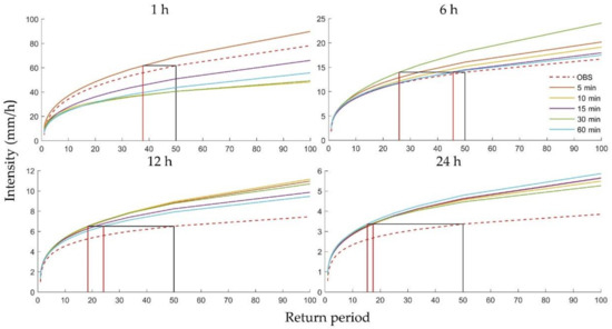
Figure 10.
Rainfall intensity of the historical and future climate based on five types of downscaling results for 1, 6, 12, and 24 h for different return periods at Wattisham station.
It should be noted that there is no guarantee that the NPRED-MoF downscaling method will completely eliminate uncertainty. Rather, this comparative experiment was designed to explore the impact of the NPRED-MoF downscaling method on the uncertainty of IDF curves.
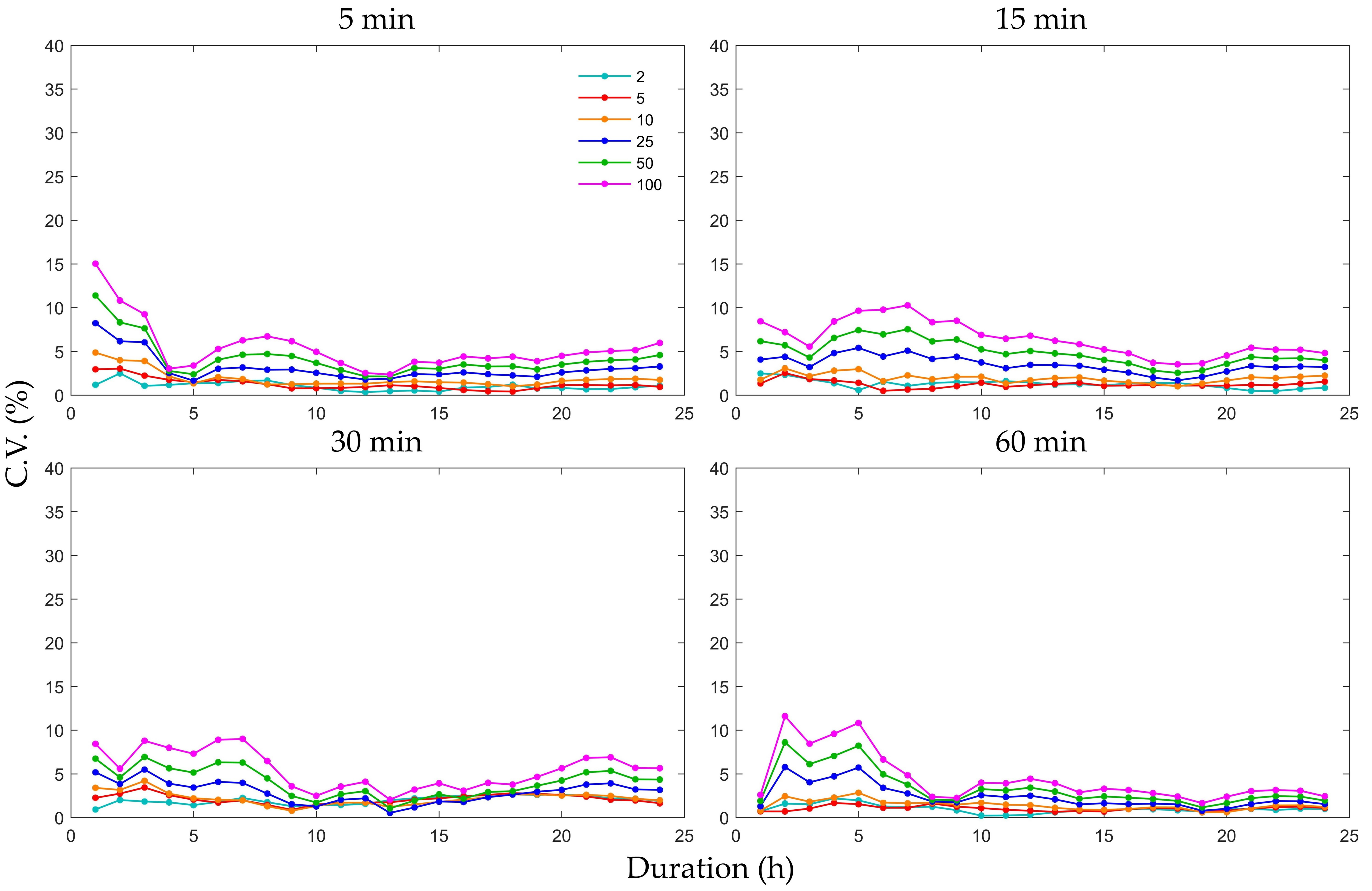
The C.V. distributions of the rainfall intensity, with the downscaling procedure implemented five times, for six return periods and 24 durations are presented in Figure 11. Each subplot is based on one of the fixed downscaling scales. The C.V. values for shorter durations were larger than those for the longer durations and were below 10% for most values; however, the downward trends were not pronounced. Regardless, the uncertainty increased as the return period lengthened. Comparing the first plot in Figure 8 with each plot in Figure 11, the C.V. in the latter was much smaller than that of the former for shorter durations, suggesting that uncertainties due to downscaling ratios are much greater than those due to the downscaling method for these durations. However, the values in Figure 11 were not invariably smaller than those in the first subplot in Figure 8 as the duration lengthened, implying that it might not be possible to clearly identify the source of this uncertainty for longer durations. Nevertheless, most of these C.V. values were below 5%, which is sufficiently low to neglect the corresponding uncertainty. Therefore, the durations for which the uncertainty cannot be neglected are mainly those affected by the downscaling ratio.
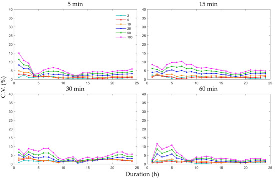
Figure 11.
Coefficient of variation (C.V.) distributions of the rainfall intensity of the downscaling procedure implemented five times for six return periods and 24 durations for Heathrow station; each plot is based on one fixed downscaling scale.
4.3. IDF Curves for Different RCM Ensemble Members
We obtained the IDF curves for all 11 RCM ensemble members to rule out differences in the data stemming from the use of only one particular ensemble member. Figure 12 shows the IDF curves for the historical (red dotted line) and future (11 solid lines) climates for five return periods for Heathrow station. The IDF curves show an obvious increase in both intensity and frequency for future storms compared to the historical data from the subplots in Figure 12. The future IDF curves were more compact for shorter return periods for each time scale and appeared to have a parallel linear relationship that was more pronounced for the shorter return periods for each scale. The other stations also had similar patterns.
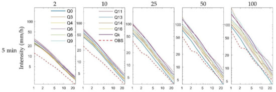
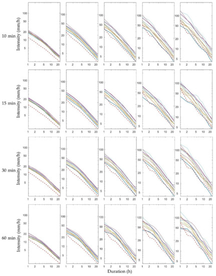
Figure 12.
IDF curves for historical (red dotted line) and future (solid lines) climate data for historical rainfall data from Heathrow station and modelled rainfall results from five downscaling ratios of 11 RCM ensemble members. Each solid line represents a specific returning period and 24 rainfall durations and is based on a specific downscaling radio and RCM ensemble.
Table 5 and Table 6 show the mean and C.V. of rainfall intensity for Heathrow station for the 11 ensemble members for three durations (1, 6, and 24 h) and three return periods (2, 10, and 100 years), listed in descending order of the total rainfall intensity. In most cases, the C.V. values were greater than 15% for the 1 h durations, indicative of notable uncertainty of the IDF curves for all 11 RCM ensemble members for shorter durations. Although most C.V. values were below 5% for the 6 h and 24 h durations for the 1 year and 10 years return periods, the C.V. increased to 16.49% and 11.26% for the 100 years return period for the 6 h and 12 h durations, respectively. For all RCM ensemble members in Table 6, the C.V. values were consistently greater for the 1 h duration than the 6 h and 12 h durations, and the C.V. values increased according to the lengthening return periods in a similar manner. These results demonstrate that the patterns in scale-driven uncertainty examined in Section 4.2 hold for all RCM ensemble members.

Table 5.
Mean rainfall intensity (mm/h) based on the downscaling results using the five time scales of 11 RCM ensemble members for three return periods and three durations for Heathrow station.

Table 6.
C.V. (%) of rainfall intensity based on the downscaling results using five time scales of 11 ensemble members for three return periods and three durations for Heathrow station.
Table 5 further confirms the nearly parallel linear relationships between the 11 RCM ensemble members. The maximum or minimum mean values of the storm intensity for each return period appear in the same row in Table 5, but, interestingly, the maximum or minimum C.V. values appear in different rows in Table 6. Furthermore, most of the maximum or minimum mean values and the C.V. values belong to different RCM ensemble members for each return period and duration, suggesting that there was no linear or other apparent relationship between the C.V. values and the mean values of different RCM ensemble members. This shows that the scale-driven uncertainty of the IDF curves is irrelevant to the mean size of the storm intensity of different RCM ensemble members for particular durations and return periods.
5. Conclusions
In this study, we explored the uncertainty in future IDF curves caused by downscaling RCM data and quantified the uncertainty using a series of future climate IDF curves obtained by downscaling the temporal resolution of data from four stations in the UK and 11 RCM ensemble members. This was performed using DBS bias-correction technology and NPRED-MoF statistical downscaling methods.
The differences in the IDF curves stemming from the five-step downscaling process indicated that the scales had a significant impact on the uncertainty of the IDF curves and that these were too great to be neglected, especially for shorter durations and longer return periods. For instance, the SD and C.V. of rainfall intensity at different time scales reached as high as 14.68 mm/h and 30.42%, respectively, based on records from Heathrow station when the duration was 1 h and the return period was 50 years. The results can be summarized as follows: (1) the scale-induced uncertainty in future IDF curves decreased significantly as the duration of each return period increased despite the presence of turning points (between 5 and 10 h), after which the uncertainty fluctuated below a consistent value (a C.V. of less than 5%, in most cases); (2) the uncertainty increased as the return period lengthened for each duration and it was more pronounced for shorter (1 or 2 h) durations; and (3) the patterns or trends of scale-driven uncertainties in IDF curves were similar across the 11 RCM ensemble members, and the former showed no obvious correlations between the mean storm intensity for different RCM ensemble members for each duration and return period.
These results indicate that the uncertainty in IDF curves stemming from downscaling ratios is of critical significance, and this study presents a method to better understand this uncertainty. Considering that uncertainties in IDF curves could be propagated or enlarged through their use in hydrometeorological applications, the results demonstrate that IDF curves based on a one-step downscaling process are unreliable. This could result in doubts over the security and reliability of the design of water facilities, such as urban drainage networks or dams, if they are based on future IDF curves that do not consider multiple scales. This suggests that IDF curves should be developed based on multiplying various time scales and averaging the results; however, more theoretical support is required. Human security and health, which is dependent on such basic infrastructure, could be in danger if put at risk if the infrastructure were designed based on IDF curves with high uncertainty values. Therefore, it is necessary to invent a downscaling method that considers the uncertainties caused by temporal downscaling in source data used in modeling.
This study determined, quantified, and analyzed the scale-driven uncertainty of IDF curves. However, it neither sought the mechanism driving this uncertainty nor found a way to solve it. What will the scale-induced uncertainty be in future IDF curves if we adopt methods that utilize multiple-process downscaling? More significantly, how does the scale-driven uncertainty propagate in hydrometeorological applications? Thus, future studies should identify factors driving the uncertainties and design a framework to reduce them or to invent a downscaling method that considers the uncertainty stemming from downscaling data of different time scales. Further studies could characterize this uncertainty by combining multiple downscaling methods. The rules by which uncertainty propagates in hydrometeorological applications will also be explored in future research.
Acknowledgments
This study is supported by Newton Fund via Natural Environment Research Council (NERC) and Economic and Social Research Council (ESRC) (NE/N012143/1), and the National Natural Science Foundation of China (Nos: 41771424, 41501429), and University Natural Science Project of Jiangsu Province (No: 16KJA170001). The authors would like to thank the British Atmospheric Data Centre, the Environment Agency, and the UK Met Office for providing the data sets used in this study.
Author Contributions
Qiqi Yang was responsible for the literature search, setting up the experiments, completing most of the experiments, and writing the initial draft of the manuscript. Qiang Dai, Dawei Han, and Shuliang Zhang principally conceived the idea for the study, the design of the study and provided financial support. Xuehong Zhu contributed to figures.
Conflicts of Interest
The authors declare no conflict of interest.
References
- Cheng, L.; AghaKouchak, A. Nonstationary precipitation intensity-duration-frequency curves for infrastructure design in a changing climate. Sci. Rep. 2014, 4, 7093. [Google Scholar] [CrossRef] [PubMed]
- Pui, A.; Sharma, A.; Mehrotra, R.; Sivakumar, B.; Jeremiah, E. A comparison of alternatives for daily to sub-daily rainfall disaggregation. J. Hydrol. 2012, 470–471, 138–157. [Google Scholar] [CrossRef]
- Sarhadi, A.; Soulis, E.D. Time-varying extreme rainfall intensity-duration-frequency curves in a changing climate. Geophys. Res. Lett. 2017, 44. [Google Scholar] [CrossRef]
- Chen, Y.R.; Chu, P.S. Trends in precipitation extremes and return levels in the Hawaiian islands under a changing climate. Int. J. Climatol. 2014, 34, 3913–3925. [Google Scholar] [CrossRef]
- Madsen, H.; Lawrence, D.; Lang, M.; Martinkova, M.; Kjeldsen, T. Review of trend analysis and climate change projections of extreme precipitation and floods in Europe. J. Hydrol. 2014, 519, 3634–3650. [Google Scholar] [CrossRef]
- Wang, W.; Zhou, W.; Fong, S.K.; Leong, K.C.; Tang, I.M.; Chang, S.W.; Leong, W.K. Extreme rainfall and summer heat waves in Macau based on statistical theory of extreme values. Clim. Res. 2015, 66, 91–101. [Google Scholar] [CrossRef]
- Koutsoyiannis, D.; Kozonis, D.; Manetas, A. A mathematical framework for studying rainfall intensity-duration-frequency relationships. J. Hydrol. 1998, 206, 118–135. [Google Scholar] [CrossRef]
- Mirhosseini, G.; Srivastava, P.; Stefanova, L. The impact of climate change on rainfall intensity–duration–frequency (IDF) curves in Alabama. Reg. Environ. Chang. 2013, 13, 25–33. [Google Scholar] [CrossRef]
- Panthou, G.; Vischel, T.; Lebel, T.; Blanchet, J.; Quantin, G.; Ali, A. Extreme rainfall in west Africa: A regional modeling. Water Resour. Res. 2012, 48, 682–688. [Google Scholar] [CrossRef]
- Lehmann, E.A.; Phatak, A.; Stephenson, A.; Lau, R. Spatial modelling framework for the characterisation of rainfall extremes at different durations and under climate change. Environmetrics 2016, 27, 239–251. [Google Scholar] [CrossRef]
- Yilmaz, A.G.; Perera, B.J.C. Extreme rainfall nonstationarity investigation and intensity–frequency–duration relationship. J. Hydrol. Eng. 2014, 19, 1160–1172. [Google Scholar] [CrossRef]
- Agilan, V.; Umamahesh, N.V. Is the covariate based non-stationary rainfall IDF curve capable of encompassing future rainfall changes? J. Hydrol. 2016, 541, 1441–1455. [Google Scholar] [CrossRef]
- Lima, C.H.R.; Kwon, H.-H.; Kim, J.-Y. A bayesian β distribution model for estimating rainfall IDF curves in a changing climate. J. Hydrol. 2016, 540, 744–756. [Google Scholar] [CrossRef]
- Srivastav, R.K.; Schardong, A.; Simonovic, S.P. Equidistance quantile matching method for updating IDF curves under climate change. Water Resour. Manag. 2014, 28, 2539–2562. [Google Scholar] [CrossRef]
- Fadhel, S.; Rico-Ramirez, M.A.; Han, D. Uncertainty of intensity–duration–frequency (IDF) curves due to varied climate baseline periods. J. Hydrol. 2017, 547, 600–612. [Google Scholar] [CrossRef]
- Willems, P.; Arnbjerg-Nielsen, K.; Olsson, J.; Nguyen, V.T.V. Climate change impact assessment on urban rainfall extremes and urban drainage: Methods and shortcomings. Atmos. Res. 2012, 103, 106–118. [Google Scholar] [CrossRef]
- Nazemi, A.-R.; Elshorbagy, A.; Pingale, S. Uncertainties in the estimation of future annual extreme daily rainfall for the city of Saskatoon under climate change effects. In Proceedings of the 20th Canadian Hydrotechnical Conference, Ottawa, ON, Canada, 14–17 June 2011. [Google Scholar]
- Kim, K.B.; Kwon, H.-H.; Han, D. Bias correction methods for regional climate model simulations considering the distributional parametric uncertainty underlying the observations. J. Hydrol. 2015, 530, 568–579. [Google Scholar] [CrossRef]
- Chandra, R.; Saha, U.; Mujumdar, P.P. Model and parameter uncertainty in IDF relationships under climate change. Adv. Water Resour. 2015, 79, 127–139. [Google Scholar] [CrossRef]
- Chen, J.; Brissette, F.P.; Leconte, R. Uncertainty of downscaling method in quantifying the impact of climate change on hydrology. J. Hydrol. 2011, 401, 190–202. [Google Scholar] [CrossRef]
- Gobiet, A.; Kotlarski, S.; Beniston, M.; Heinrich, G.; Rajczak, J.; Stoffel, M. 21st century climate change in the European alps—A review. Sci. Total Environ. 2014, 493, 1138–1151. [Google Scholar] [CrossRef] [PubMed]
- Chan, S.C.; Kendon, E.J.; Fowler, H.J.; Blenkinsop, S.; Roberts, N.M. Projected increases in summer and winter UK sub-daily precipitation extremes from high-resolution regional climate models. Environ. Res. Lett. 2014, 9, 084019. [Google Scholar] [CrossRef]
- Ekström, M.; Fowler, H.J.; Kilsby, C.G.; Jones, P.D. New estimates of future changes in extreme rainfall across the UK using regional climate model integrations. 2. Future estimates and use in impact studies. J. Hydrol. 2005, 300, 234–251. [Google Scholar] [CrossRef]
- Met Office; NCAS British Atmospheric Data Centre. MIDAS UK Hourly Rainfall Data. 2006. Available online: http://catalogue.ceda.ac.uk/uuid/bbd6916225e7475514e17fdbf11141c1 (accessed on 11 November 2017).
- Met Office; NCAS British Atmospheric Data Centre. MIDAS UK Daily Temperature Data. 2006. Available online: http://catalogue.ceda.ac.uk/uuid/1bb479d3b1e38c339adb9c82c15579d8 (accessed on 11 November 2017).
- Coles, S.; Bawa, J.; Trenner, L.; Dorazio, P. An Introduction to Statistical Modeling of Extreme Values; Springer: London, UK, 2001; Volume 208. [Google Scholar]
- Hadley Centre for Climate Prediction and Research; NCAS British Atmospheric Data Centre. UKCP09: Met Office HadRM3-PPE UK Model Runs. 2014. Available online: http://catalogue.ceda.ac.uk/uuid/465ecd8a305ffb9df2bd8b54cada669f (accessed on 5 November 2017).
- Dai, Q.; Han, D.; Rico-Ramirez, M.; Srivastava, P.K. Multivariate distributed ensemble generator: A new scheme for ensemble radar precipitation estimation over temperate maritime climate. J. Hydrol. 2014, 511, 17–27. [Google Scholar] [CrossRef]
- Dai, Q.; Han, D.; Rico-Ramirez, M.A.; Zhuo, L.; Nanding, N.; Islam, T. Radar rainfall uncertainty modelling influenced by wind. Hydrol. Process. 2015, 29, 1704–1716. [Google Scholar] [CrossRef]
- Yang, W.; Andréasson, J.; Phil Graham, L.; Olsson, J.; Rosberg, J.; Wetterhall, F. Distribution-based scaling to improve usability of regional climate model projections for hydrological climate change impacts studies. Hydrol. Res. 2010, 41, 211. [Google Scholar] [CrossRef]
- Olsson, T.; Jakkila, J.; Veijalainen, N.; Backman, L.; Kaurola, J.; Vehviläinen, B. Impacts of climate change on temperature, precipitation and hydrology in Finland—Studies using bias corrected regional climate model data. Hydrol. Earth Syst. Sci. 2015, 19, 3217–3238. [Google Scholar] [CrossRef]
- Husak, G.J.; Michaelsen, J.; Funk, C. Use of the gamma distribution to represent monthly rainfall in Africa for drought monitoring applications. Int. J. Climatol. 2007, 27, 935–944. [Google Scholar] [CrossRef]
- Piani, C.; Haerter, J.O.; Coppola, E. Statistical bias correction for daily precipitation in regional climate models over Europe. Theor. Appl. Climatol. 2009, 99, 187–192. [Google Scholar] [CrossRef]
- Sharma, A.; Mehrotra, R.; Li, J.; Jha, S. A programming tool for nonparametric system prediction using partial informational correlation and partial weights. Environ. Model. Softw. 2016, 83, 271–275. [Google Scholar] [CrossRef]
- Sharma, A.; Mehrotra, R. An information theoretic alternative to model a natural system using observational information alone. Water Resour. Res. 2014, 50, 650–660. [Google Scholar] [CrossRef]
- Mehrotra, R.; Westra, S.; Sharma, A.; Srikanthan, R. Continuous rainfall simulation: 2. A regionalized daily rainfall generation approach. Water Resour. Res. 2012, 48. [Google Scholar] [CrossRef]
- Westra, S.; Mehrotra, R.; Sharma, A.; Srikanthan, R. Continuous rainfall simulation: 1. A regionalized subdaily disaggregation approach. Water Resour. Res. 2012, 48. [Google Scholar] [CrossRef]
- Sharif, M.; Burn, D.H. Improved k-nearest neighbor weather generating model. J. Hydrol. Eng. 2007, 12, 42–51. [Google Scholar] [CrossRef]
© 2018 by the authors. Licensee MDPI, Basel, Switzerland. This article is an open access article distributed under the terms and conditions of the Creative Commons Attribution (CC BY) license (http://creativecommons.org/licenses/by/4.0/).

