1. Introduction
Many areas of the United States (U.S.) are trying to achieve the current National Ambient Air Quality Standards (NAAQS) attainment level for ozone. Ozone formation is linked to emissions of volatile organic compounds (VOCs) and nitrogen oxides (NO
x) [
1]. The chemistry leading to ozone production from emissions of VOC and NO
x is non-linear [
2]. Contour plots of ozone versus NO
x and VOC emissions (ozone isopleths) are often employed to illustrate the non-linear response of ozone levels to NO
x and VOC changes, and have been used in the past in the empirical kinetic modeling approach (EKMA) developed by the U.S. Environmental Protection Agency (EPA) to develop control strategies for ozone reduction [
3]. Thus, the isopleths of ozone versus VOC and NO
x emissions are often referred to as EKMA diagrams. The EKMA generates ozone isopleths for specific monitors in a city. Once the maximum measured ozone concentration at a monitor has been identified, the VOC and NO
x reductions needed to achieve the NAAQS level are determined using the EKMA from the distance along the VOC and NO
x axes to the isopleth that represents the desired peak ozone concentration mandated by the NAAQS. The abundance of VOCs relative to NO
x is characterized by the VOC/NO
x ratio. The VOC/NO
x ratio is important in the behavior of the VOC-NO
x-ozone system and has a major effect on how reductions in VOC and NO
x affect ozone concentrations [
4].
While the EKMA for regulatory planning has been superseded by photochemical grid modeling, the ozone isopleths are useful for understanding how ozone levels at a particular location may respond to reductions in NO
x, VOC, or both. The objective of this study was to develop future-year (2030) VOC-NO
x isopleth diagrams of the 4th highest maximum daily 8-h average (H4MDA8) ozone design value concentrations (DVC) at monitors of interest in the South Coast Air Basin (SoCAB) and San Joaquin Valley (SJV) in California, and in Maryland. These areas were selected to illustrate contrasting current ozone classification levels: SoCAB and SJV at extreme or severe [
5], and Maryland at moderate or marginal [
6]. Regions where ozone production is limited by the presence of nitrogen oxides or hydrocarbons are readily apparent in such a diagram [
7]. The Comprehensive Air Quality Model with Extensions (CAMx) version 6.4 [
8] is the latest version of the photochemical grid model (PGM) and was used to conduct several brute force scenarios. The CAMx allows for integrated “one-atmosphere” assessments of tropospheric air pollution (ozone, particulates, air toxics) over spatial scales ranging from neighborhoods to continents. It is a “state-of-the-science” open-source system that is computationally efficient, flexible, and publicly available. Meteorological fields are supplied to the CAMx from separate, commonly used weather prediction models such as the Weather Research and Forecasting (WRF) model. All emission inputs are supplied from external pre-processing systems. The CAMx simulates the emission, dispersion, chemical reaction, and removal of pollutants by marching the Eulerian continuity equation forward in time for each chemical species in a system of nested three-dimensional grids. The ozone isopleths developed in this study using the CAMx were compared with the South Coast Air Quality Management District (SCAQMD) 2016 Air Quality Management Plan (AQMP) [
9] isopleths, which were generated with the U.S. EPA photochemical grid model, the Community Multiscale Air Quality (CMAQ) [
10,
11].
2. Method
In previous modeling studies, Collet et al. [
12,
13] simulated the entire contiguous U.S. (continental U.S. or CONUS) domain (396 vertical by 246 horizontal grid cells) at 12-km resolution with the CAMx 6.4. For this study, a different approach was adopted because the development of ozone isopleths relating ozone responses to NO
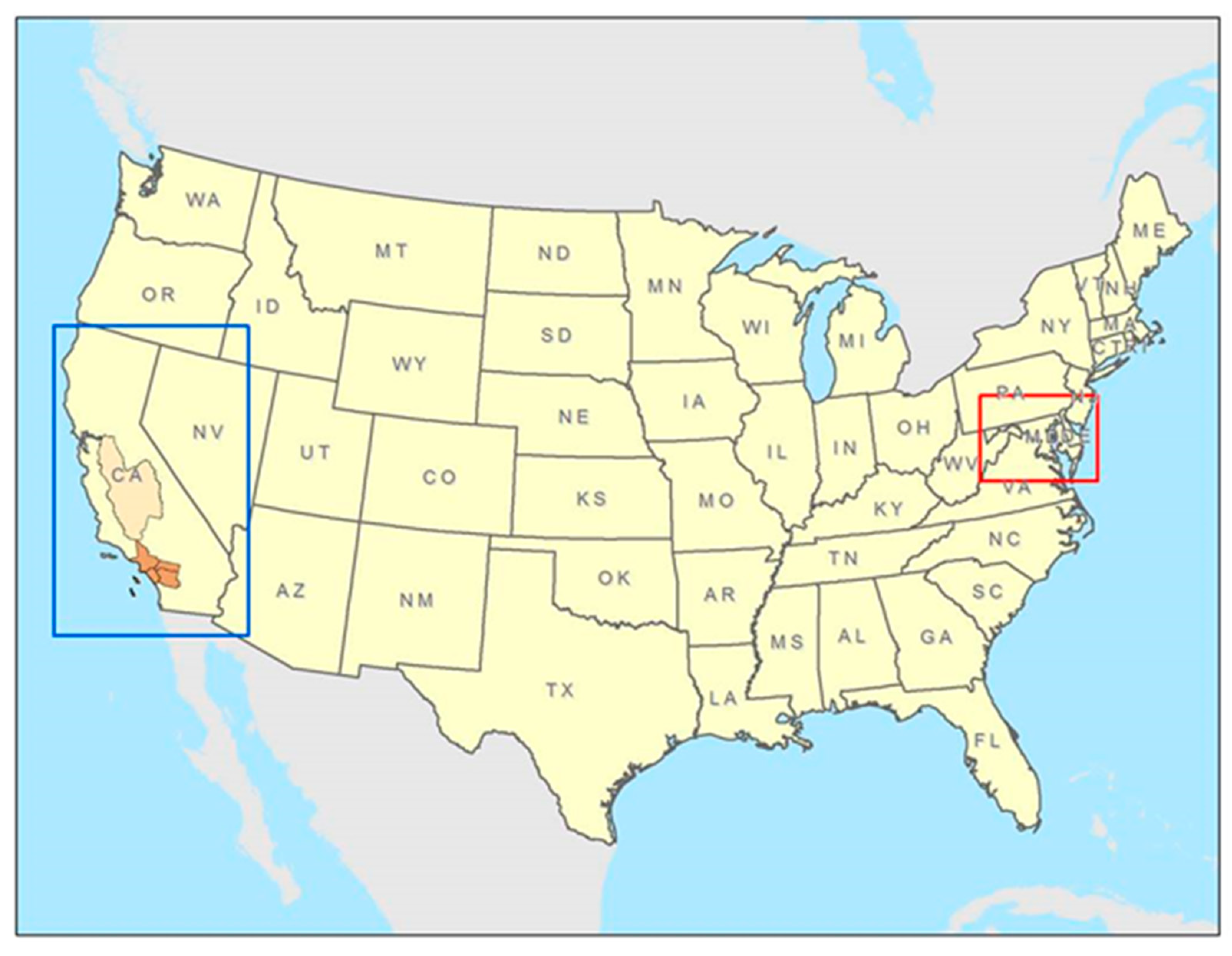
x and VOC emissions changes required several tens of emissions scenario simulations to be conducted. This approach, referred to as brute force sensitivity analyses, is impractical for the large CONUS domain, since it is time- and resource-intensive. Since the objective of this study was to develop ozone isopleth diagrams for specific sub-regions of the country, sub-regional CAMx simulations were conducted to achieve the study objective. Specifically, the emissions scenario simulations were conducted for two subdomains using 12 km by 12 km grid resolution, one in the Western U.S. and the second in the Eastern U.S.
Figure 1 shows the two subdomains within the outer CONUS domain. The western subdomain (66 vertical by 105 horizontal grid cells) covers most of California and includes the SoCAB and SJV, while the eastern subdomain (40 vertical by 29 horizontal grid cells) covers Maryland and portions of the surrounding states.
The existing CAMx modeling databases used by Collet et al. [
13] were developed for the CONUS domain. For that study, the 2025 CMAQ-ready emissions provided by the EPA were used for the future-year (2030) emissions. Future-year emissions from the natural source categories were assumed to be the same as the 2011 base-year emissions. The 2030 emissions for all anthropogenic source categories, except on-road mobile sources, were assumed to be the same as the EPA’s 2025 emissions case. The on-road mobile emissions for 2030 were developed using MOVES 2014 and the California Air Resources Board’s (CARB) EMFAC2014 models. It was necessary to develop new inputs for the two subdomains shown in
Figure 1. The inputs for this study consist of the following: meteorology, emissions, land use, ozone column and photolysis rates, and boundary conditions. The gridded subdomain meteorological fields and land use data were developed by extracting (“windowing”) the subdomain data from the corresponding CONUS files. Ozone column and photolysis rate data were developed as new inputs for the subdomains. Boundary conditions for the subdomains were developed by first conducting base-year (2011) and future-year (2030) CONUS domain simulations in which the 3-dimensional (3-D) concentration outputs were saved, and then windowing these outputs for the subdomains.
The 2030 future-year emissions for the CONUS domain from the Collet et al. [
13] study were windowed for the two subdomains in the Western and Eastern U.S. In that study, the 2030 future-year emissions were based on the 2025 projected emissions from the EPA 2011v6.2 platform and 2030 on-road mobile emissions generated using the latest on-road emission models. To perform the emission scenario simulations required for generating the ozone isopleths, the emissions within the sub-regions of interest (the two air basins in the western subdomain and the state of Maryland in the eastern subdomain) were adjusted. These adjustments were made using cell masks created by ArcGIS [
14] that only mark the cells within the two air basins and the Maryland state boundary. A set of reduction factors (20%, 40%, 60%, and 80%) was applied to emissions of NO
x (NO, NO
2, HONO), anthropogenic VOCs (i.e., excluding isoprene, monoterpene, and sesquiterpene emissions), and CO in grid cells identified by the cell masks, resulting in a total of 25 emission scenarios, including the base emission scenario (0% reduction), for each subdomain.
The air quality modeling was conducted using the most recent version (6.4) of the CAMx with the CB6r4 chemical mechanism. The base-year (2011) and future-year (2030) simulations for the CONUS domain were conducted with the CAMx to develop boundary conditions for the 2011 and 2030 subdomain simulations. A 10-day spin-up period was used for the two CONUS domain simulations.
A total of 52 CAMx simulations were conducted for the ozone season (1 May to 30 September) for the two subdomains. These simulations consisted of a base-year simulation and 25 future-year simulations for each of the two subdomains. The base-year results are required to calculate future-year ozone design values for the California air basins and the state of Maryland using EPA’s Modeled Attainment Test Software (MATS). The base-year subdomain simulations and the future-year subdomain simulations used a 5-day period for spin-up. The 25 future-year emission scenario calculations correspond to a 5 by 5 matrix of future-year emissions (20%, 40%, 60%, 80%, and 100% NOx emissions by 20%, 40%, 60%, 80%, and 100% VOC and CO emissions).
3. Results
Following EPA guidance, the outputs of the base-year and future-year subdomain simulations were processed using EPA’s MATS to project future-year design values (DVF) at monitoring locations of interest. Briefly, the modeling results are used in a relative sense to scale observed site-specific 8-h ozone concentrations for current-year design values (DVC) based on the relative changes in the modeled 8-h ozone concentrations between the current and future years. The model-derived scaling factors are called relative response factors (RRFs), and are based on the relative changes in the modeling results between the current-year (2011) base case and the future-year (2030) emission scenarios. This is the recommended regulatory approach to determine future-year ozone design values, and is based on the assumption that the model can predict ozone responses to changes in emissions more accurately than it can predict absolute ozone concentrations.
Table 1 and
Table 2 show the ozone NAAQS attainment status (70 ppb H4MDA8) for the three study areas without any additional controls.
Table 1 provides the list of monitors in the two California air basins and state of Maryland where future-year ozone design values were calculated using the air quality modeling results and MATS, and the future-year ozone design values at these monitors.
Table 2 quantifies the number of monitors in
Table 1 which are in or not in attainment.
A matrix of 25 (5 × 5) future-year emission scenarios for each subdomain provides 25 future-year ozone design values at the selected monitors as a function of NO
x and VOC emissions in the air basins of interest. This is a relatively coarse resolution, so it is necessary to use an interpolation technique, such as kriging, to obtain smooth contours of the ozone design values (ozone isopleths). Kriging is an advanced geostatistical procedure that generates an estimated surface from a scattered set of points. Although kriging was developed originally for applications in geostatistics, it is a general method of statistical interpolation that can be applied within any discipline to sampled data from random fields. It differs from simpler interpolation methods in that it uses the spatial correlation between sampled points to interpolate the values in the spatial field. Kriging has been used in other studies to develop ozone response surfaces [
15,
16]. PyKrige, a Python kriging library, was used for this purpose in the present study. The interpolation was performed using ordinary kriging, which is the most commonly used kriging algorithm and produces interpolation values by relying on an unknown mean value, allowing local influences due to nearby neighboring values. The original 5 × 5 matrix of values were interpolated to 81 × 81 data points, representing reductions in anthropogenic emissions in the California air basins and state of Maryland in increments of 1% from 0% to 80%. Standard Python libraries were then used to prepare the ozone isopleths.
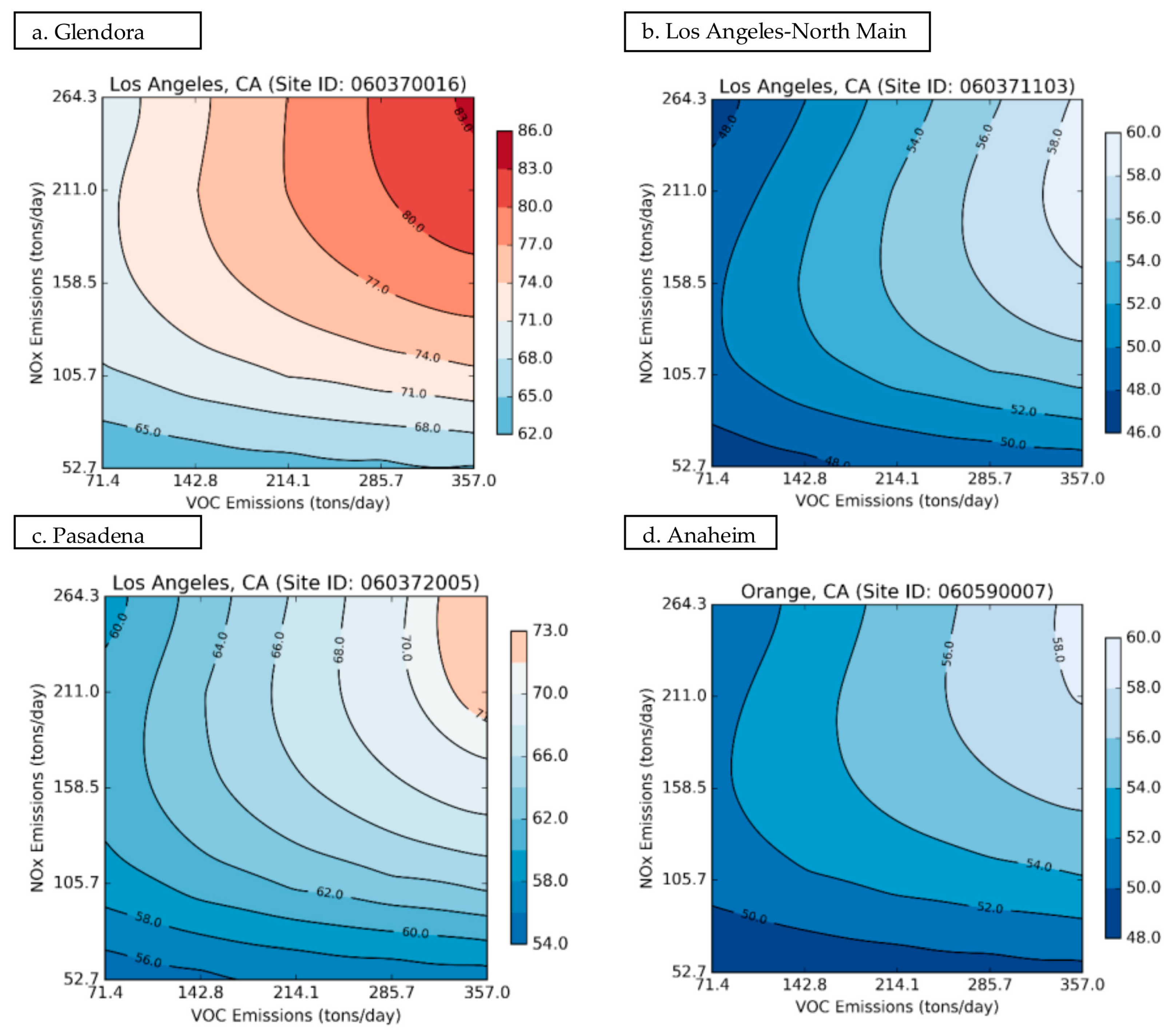
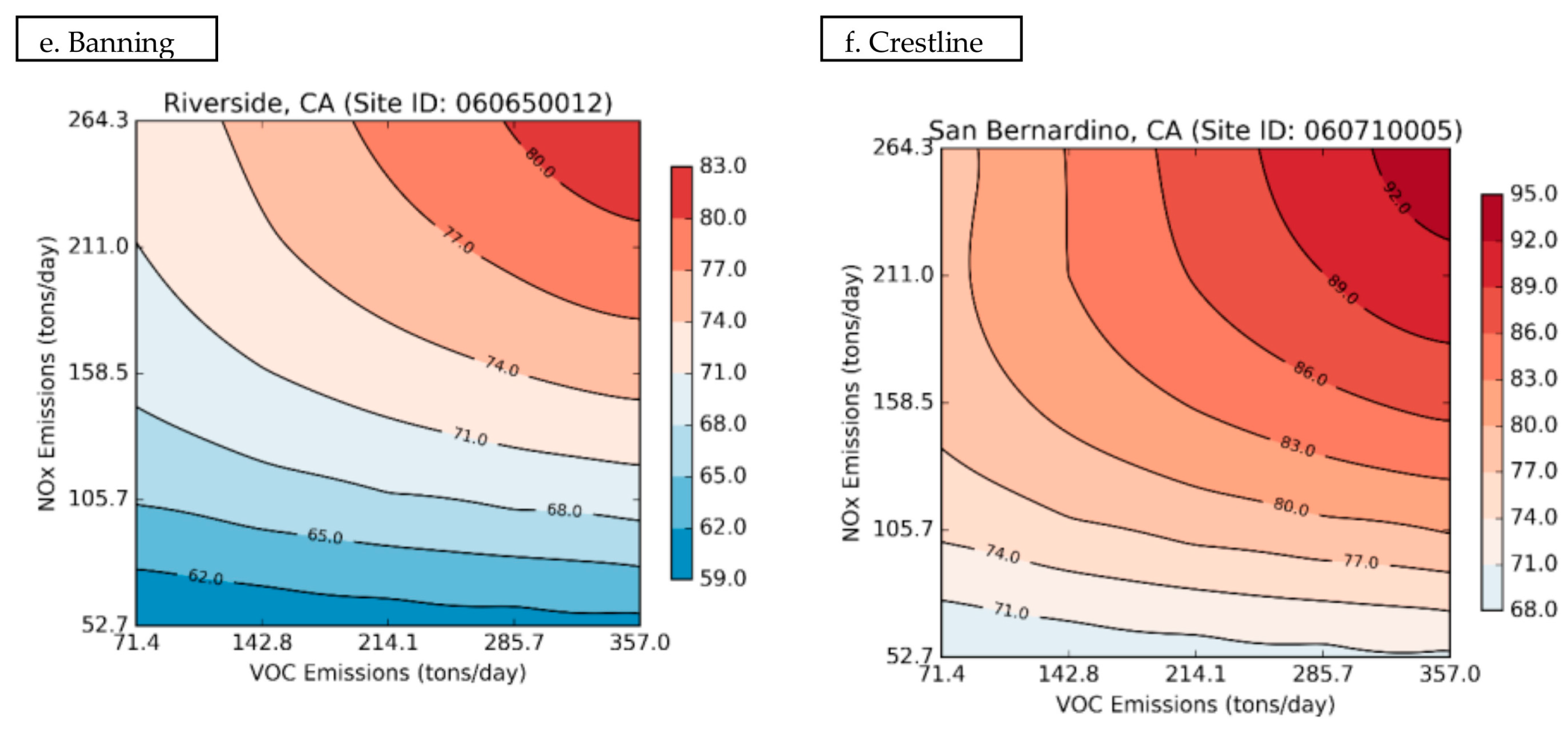
Ozone isopleths (“EKMA diagrams”) for the selected monitors in the South Coast Air Basin are shown in
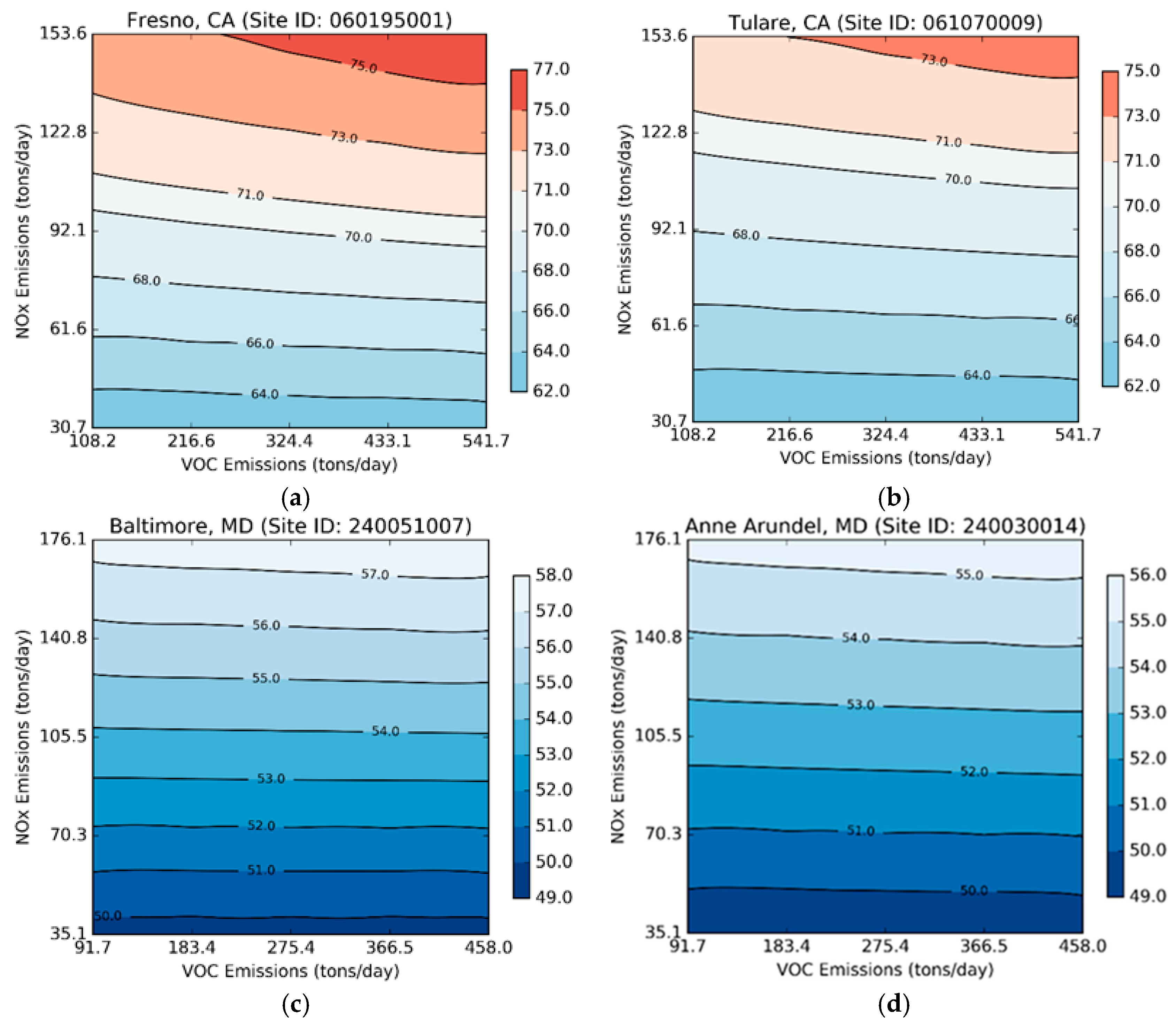
Figure 2, while
Figure 3 shows ozone isopleths for selected monitors in Fresno and Tulare, CA, and the state of Maryland. The x-axis shows the VOC anthropogenic emissions, and the y-axis the NO
x anthropogenic emissions. Thus, the y-axis and x-axis represent anthropogenic emissions ranging from 20% to 100% of the base future-year air basin anthropogenic emissions (i.e., each tick mark represents 20%). Therefore, the 2030 DVF is at the 100% NO
x and 100% VOC point, in the top right corner of the diagram. The color scheme for the ozone design values ranges from dark brown (85 ppb and higher) to dark blue (55 ppb and lower). The light blue region represents a level of about 70 ppb and provides a measure of the reductions in NO
x and/or VOC required to reach attainment at a specific monitor.
4. Discussion
Table 3 provides the future-year projected NO
x and VOC emission totals for the non-attainment areas, and the estimated NO
x or VOC emission levels needed to attain the standards in tons/day and as a reduction percentage of the base future-year emissions. In the SoCAB, 3 of the 11 monitors (West Los Angeles, Los Angeles-North Main, and Anaheim) showed attainment of the 2015 ozone NAAQS level at projected 2030 SoCAB anthropogenic emissions without further controls.
Table 3 shows that monitors in Glendora and Pasadena could meet the NAAQS with NO
x or VOC reductions, while on a percentage basis, less NO
x reductions are required than VOC reductions. Moving eastward in the SoCAB, VOC reductions to 80% will not reduce ozone to the NAAQS level. In Riverside, NO
x reductions are projected to bring the area into compliance. The northwest and most eastern areas of the SoCAB (i.e., Santa Clarita, Reseda, Crestline, and San Bernardino) are not projected to achieve compliance with 80% NO
x or VOC anthropogenic reductions. In the SJV area, four of seven monitors show attainment of the 2015 NAAQS level at projected 2030 anthropogenic emissions without further controls. To achieve attainment at the two monitors projecting non-attainment in the SJV (Fresno and Tulare), NO
x reductions would be effective, while VOC reductions would not be useful. At all the Maryland monitors, future-year ozone levels are in attainment of the 2015 NAAQS level without further controls. The Maryland area is sensitive to changes in NO
x and shows little to no sensitivity to VOC changes.
To compare this study’s ozone isopleths to those reported in the SCAQMD 2016 AQMP [
9], the modeling platform and domain are shown in
Table 4 for both studies.
Table 5 compares the additional reductions in future-year emission required to achieve attainment from the SCAQMD AQMP isopleths for 2031 and the 2030 isopleths from this study. For most of the monitors, the difference in the amount of NO
x or VOC (in tons/day or percent reduction) needed to achieve the ozone NAAQS level from the two sets of isopleths is within +25%. The SCAQMD AQMP isopleths show more NO
x-limited trends than the present study, possibly due to differences between the inputs and models used in the two studies (see
Table 4).
5. Conclusions
This study developed future-year (2030) VOC-NOx isopleths of H4MDA8 ozone design values at selected monitors in the SoCAB and SJV in California, and Maryland. Photochemical grid modeling for a large number of VOC and NOx emission reduction scenarios (from 0% to 80%) were conducted to develop the isopleths of ozone design values versus VOC and NOx emissions in each region. The latest version of the photochemical grid model, CAMx 6.4, was used in this modeling study.
The modeling results showed that only 27% of the selected monitors in the SoCAB would reach attainment of the 2015 ozone NAAQS level in 2030 without further controls. In the SJV, 57% of the monitors would reach attainment without further controls. All monitors in Maryland were projected to reach attainment of the 2015 ozone NAAQS level in 2030 at base projected emission levels. The ozone isopleths for the SoCAB and SJV were used to determine the amount of additional controls that would be required to attain the standards in 2030. This analysis showed that the areas in the western and central portions of the basins could achieve attainment with NOx or VOC reductions or a combination of both, while areas between the central and eastern locations could achieve attainment with NOx reductions, but VOC reductions are not useful. Monitors in the northwest and easternmost areas of the SoCAB are not predicted to achieve attainment with an additional 80%-reduction in future-year anthropogenic NOx or VOC. In the SJV, additional NOx reductions are effective in achieving attainment at the two monitors projected to be in non-attainment in 2030, while VOC reductions are not effective. The Maryland area is sensitive to changes in NOx and shows little to no sensitivity to VOC changes, but all monitors are projected to be in attainment without further controls in 2030.
The SoCAB ozone isopleths developed in this study were compared with those reported in the SCAQMD 2016 AQMP. While there are several differences between the two modeling studies, the results are qualitatively similar (within +25%) for most of the monitors in the relative amounts of additional NOx and/or VOC reductions needed to achieve the ozone NAAQS level. This study shows that monitors in five areas will not attain the 70 ppb NAAQS with up to 80% reductions in NOx or VOC, while the SCAQMD isopleths show that NOx controls are effective in bringing these areas into attainment.
The results from this study provide insight into designing potential control strategies for ozone attainment in future years in areas currently in non-attainment. Additional photochemical modeling using these strategies can then provide confirmation of the effectiveness of the controls.
Author Contributions
Conceptualization: S.C., T.K., P.K., and T.S.; Formal analysis: T.K., P.K., and T.S.; Investigation: T.K., P.K., and T.S.; Methodology: T.K., P.K., and T.S.; Project administration: S.C. and P.K.; Software: P.K.; Validation: T.K., P.K., and T.S.; Visualization: S.C. and T.K.; Writing—original draft: S.C.; Writing—review & editing: T.K., P.K., and T.S.
Funding
This research received no external funding.
Conflicts of Interest
The authors declare no conflict of interest.
References
- Haagen-Smit, A.J.; Fox, M.M. Photochemical ozone formation with hydrocarbons and automobile exhaust. J. Air Pollut. Control Assoc. 1954, 4, 105–109. [Google Scholar] [CrossRef]
- Lin, X.; Trainer, M.; Liu, S.C. On the nonlinearity of the tropospheric ozone production. J. Geophys. Res. Atmos. 1988, 93, 15879–15888. [Google Scholar] [CrossRef] [Green Version]
- Dodge, M.C. Combined Use of Modeling Techniques and Smog Chamber Data to Derive Ozone-Precursor Relationships; U.S. EPA Report No. EPA-600/3-77-001b; U.S. Environmental Protection Agency: Research Triangle Park, NC, USA, 1977.
- National Research Council. Rethinking the Ozone Problem in Urban and Regional Air Pollution; The National Academies Press: Washington, DC, USA, 1991; pp. 163–168. [Google Scholar] [CrossRef]
- EPA Green Book. California Nonattainment/Maintenance Status for Each County by Year for All Criteria Pollutants, Data Is Current as of 31 August 2018. Available online: https://www3.epa.gov/airquality/greenbook/anayo_ca.html (accessed on 4 September 2018).
- EPA Green Book. Maryland Nonattainment/Maintenance Status for Each County by Year for All Criteria Pollutants, Data Is Current as of 31 August 2018. Available online: https://www3.epa.gov/airquality/greenbook/anayo_md.html (accessed on 4 September 2018).
- American Meteorological Society. Available online: http://glossary.ametsoc.org/wiki/Ozone_isopleth_plot (accessed on 8 February 2018).
- ENVIRON. User’s Guide, Comprehensive Air Quality Model with Extensions (CAMx), Version 6.40, 2016. Available online: http://www.camx.com/files/camxusersguide_v6-40.pdf (accessed on 10 April 2017).
- SCAQMD. Final 2016 AQMP—CARB/EPA/SIP Submittal. South Coast Air Quality Management District, Appendix V: Modeling and Attainment Demonstration, Attachment 4: 2031 8-Hour Ozone Isopleths; South Coast Air Quality Management District: Diamond Bar, CA, USA, 2017; pp. 1–24.
- Byun, D.; Schere, K.L. Review of the governing equations, computational algorithms, and other components of the Models-3 Community Multiscale Air Quality (CMAQ) modeling system. Appl. Mech. 2006, 59, 51–77. [Google Scholar] [CrossRef]
- Foley, K.M.; Roselle, S.J.; Appel, K.W.; Bhave, P.V.; Plein, J.E.; Otte, T.L.; Mathur, R.; Sarwar, G.; Young, J.O.; Gilliam, R.C.; et al. Incremental testing of the Community Multiscale Air Quality (CMAQ) modeling system version 4.7. Geosci. Model Dev. 2010, 3, 205–226. [Google Scholar] [CrossRef] [Green Version]
- Collet, S.; Minoura, H.; Kidokoro, T.; Sonoda, Y.; Kinugasa, Y.; Karamchandani, P. Evaluation of Light Duty Vehicle Mobile Source Regulations on Ozone Concentration Trends in 2018 & 2030 in the Western and Eastern U.S. J. Air Waste Manag. 2014, 64, 175–183. [Google Scholar] [CrossRef]
- Collet, S.; Kidokoro, T.; Karamchandani, P.; Shah, T.; Jung, J. Future-year ozone prediction for the United States using updated models and inputs. J. Air Waste Manag. Assoc. 2017, 67, 938–948. [Google Scholar] [CrossRef] [PubMed]
- ESRI. ArcGIS Desktop: Release 10; Environmental Systems Research Institute: Redlands, CA, USA, 2011. [Google Scholar]
- Xing, J.; Wang, S.X.; Jang, C.; Zhu, Y.; Hao, J.M. Nonlinear response of ozone to precursor emission changes in China: A modeling study using response surface methodology. Atmos. Chem. Phys. 2011, 11, 5027–5044. [Google Scholar] [CrossRef]
- Cao, T.; Lin, C.J.; Yang, W.; Huang, S.; Chu, H.; Ho, T.C. Application of ABaCAS-TX for ozone non-attainment in Southeast Texas. Presented at the 16th Annual CMAS Conference, Chapel Hill, NC, USA, 23–25 October 2017. [Google Scholar]
© 2018 by the authors. Licensee MDPI, Basel, Switzerland. This article is an open access article distributed under the terms and conditions of the Creative Commons Attribution (CC BY) license (http://creativecommons.org/licenses/by/4.0/).


