A Numerical Framework for Evaluating Flood Inundation Hazard under Different Dam Operation Scenarios—A Case Study in Naugatuck River

Abstract

Worldwide, many river floodplains contain critical infrastructure that is vulnerable to extreme hydrologic events. These structures are designed based on flood frequency analysis aimed at quantifying the magnitude and recurrence of the extreme events. This research topic focuses on estimating flood vulnerability at ungauged locations based on an integrative framework consisting of a distributed rainfall–runoff model forced with long-term (37 years) reanalysis meteorological data and a hydraulic model driven by high-resolution airborne LiDAR-derived terrain elevation data. The framework is applied to a critical power infrastructure located within Connecticut’s Naugatuck River Basin. The hydrologic model reanalysis is used to derive 50-, 100-, 200-, and 500-year return period flood peaks, which are then used to drive Hydrologic Engineering Center’s River Analysis System (HEC-RAS) hydraulic simulations to estimate the inundation risk at the infrastructure location under different operation strategies of an upstream reservoir. This study illustrates the framework’s potential for creating flood maps at ungauged locations and demonstrates the effects of different water management scenarios on the flood risk of the downstream infrastructure.

1. Introduction

Floods are among the most damaging natural disasters, with increasing impact and frequency in Northeastern United States [1]. In the United States alone in recent decades floods have accounted for thousands of deaths and tens of billions of dollars in annual losses. Additionally, many utilities rely on critical infrastructure located on floodplains that are vulnerable to these extreme hydrologic events, allowing disturbances to extend beyond the floodplain. In flood resilience, we seek to quantify and mitigate the flood risk, as well as expedite recovery from the consequences after a flooding event occurs [2]. Resilience can be improved in many ways, including land use management, flood infrastructure management and operation, storm water withholding, more effective flood emergency preparedness, and flood response policy. However, before policy actions can be put in place, the risk must first be systematically quantified.

In relation to flood design, engineers use historical flow observations to derive information relative to the expected recurrence (i.e., return period) and magnitude (i.e., return level) of a flood event. The observed frequency is modeled using a probability distribution that can further be used to estimate the return period of event magnitudes that are generally unobserved (e.g., flood event with 500 years return period). Distributions used in frequency analysis vary, but in the U.S.A. engineering practice relies on the use of Log-Pearson Type III, which is recommended by the U.S. Water Resource Council [3]. Information regarding magnitude and frequency of occurrence of flooding events gathered through flood frequency analysis (FFA) is instrumental in mitigating losses associated with floods, particularly when designing hydraulic structures such as reservoirs and dams.

Hydrologists have developed a number of methods to conduct FFA. These methods can broadly be classified into two groups: statistical approaches and rainfall-runoff modeling. For statistical approaches, statistical analysis or hydrological regionalization are used to analyze hydrological data within a basin, or transfer hydrological information from one or more homogenous gauged catchments to a neighboring or geographically/hydrologically similar basin [4,5,6]. However, the quality of the estimation in the basin is subject to the continuous length of flow observations of the basin or neighboring gauged basins, and potential nonstationarity of the historical flood trend. In an alternate approach, observed precipitation combined with various other meteorological forcing parameters are used to drive physically-based hydrologic and flood routing models to simulate surface flows [7], which can have longer time spans but can be affected by the biased peak estimation. Surface flows are made up of both overland and channel flow routing, which can either be handled separately by two models [8,9], or combined through a coupled model [10,11]. Hydrodynamic routing models simulate surface flows based on solutions to simplified shallow water equations like the kinematic wave [12] or diffusion wave equations [9]. Solutions to these equations rely on parameters directly derived from physical watershed characteristics rather than empirically estimated coefficients. Specifically, physically-based distributed hydrologic models are able to capture the spatial variability of hydrologic parameters, and thereby better characterize the heterogeneity of certain complex hydrologic processes within catchments [13,14,15]. In inland watersheds, flooding is caused by rainfall, snowmelt, or a combination of both. Distributed hydrologic models have the capacity of accounting for the intra-basin variability of runoff-producing mechanisms by integrating gridded meteorological forcing with land cover, vegetation, terrain, and soil data. Furthermore, with the availability of high-resolution reanalysis forcing datasets like the North American Land Data Assimilation System (NLDAS), hydrologic models can now make use of quality controlled, temporally and spatially consistent datasets at a fine spatiotemporal resolution, often in areas that were previously uncovered by ground-based measurement networks. This study used The Coupled Routing and Excess Storage–Soil–Vegetation–Atmosphere–Snow (CREST-SVAS) model driven by NLDAS forcing data to simulate flows in basins of Northeastern United States [13].

The objective of this study is to demonstrate a numerical framework for evaluating flood vulnerability in terms of inundation at a site of interest in the Naugatuck River basin featuring critical utility infrastructure and different operation scenarios for an upstream dam. In the past, artificial intelligence (AI) has been used for the forecast of flood inundation [16,17] and dam-controlled reservoir water level [18]. Applying the AI techniques to assess flood vulnerability at this site of interest is however difficult because of the lack of necessary long-term observations at the site of interest and the existence of a major flood control dam upstream. This paper presents an integrative framework, involving atmospheric reanalysis driven hydrologic and hydraulic simulations that provide long-term flow data based FFA, and examine the impact of dam operation on the downstream floodplain under varying flood return periods.

2. Materials and Methods

2.1. Study Area

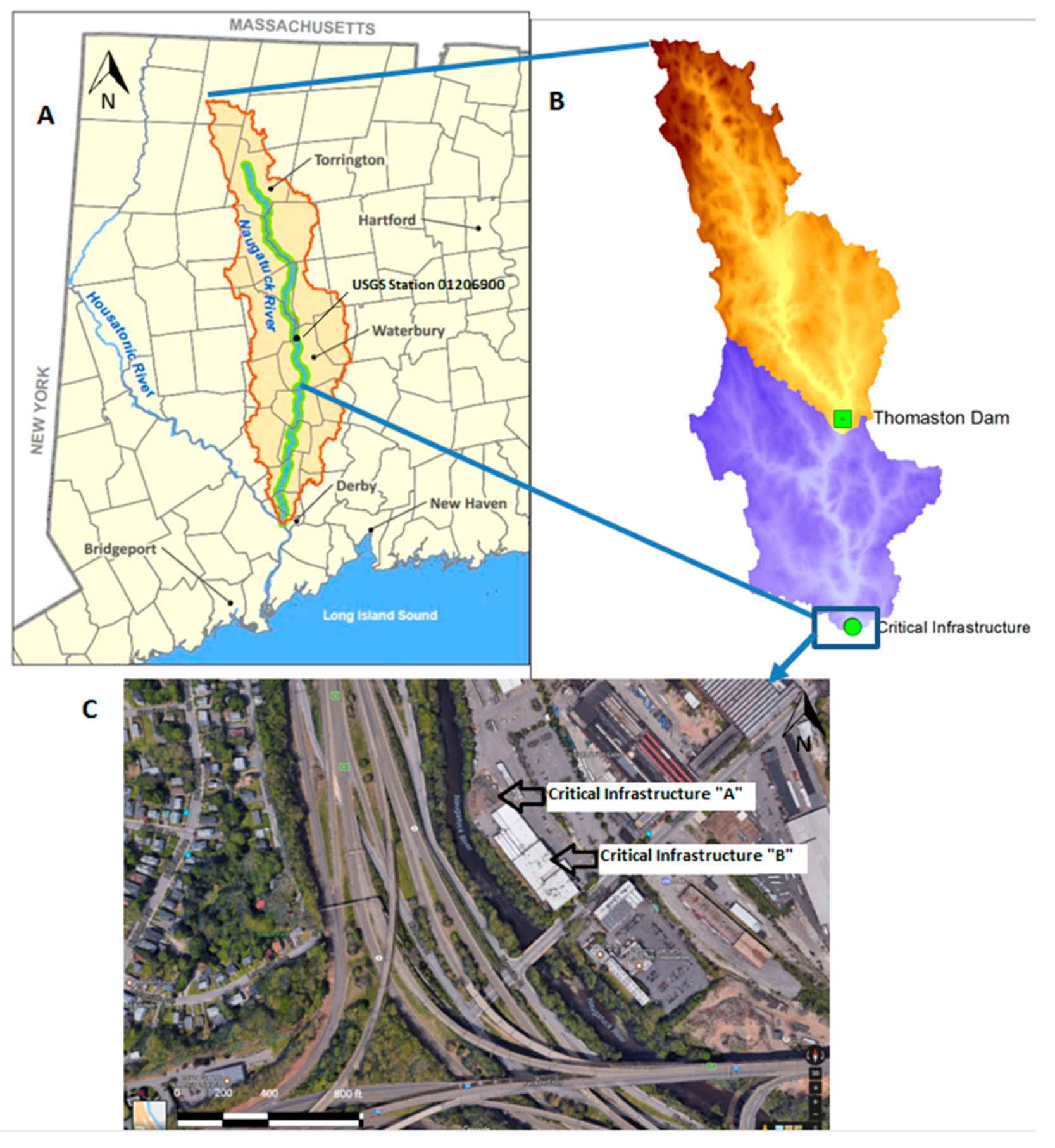
Located in Western Connecticut, the Naugatuck River is the largest tributary of the Housatonic River. Entirely confined within the state’s borders, the Naugatuck River spans over 63 km south from Torrington to Derby, 19 km north of the Long Island Sound. The stream features quick flows for the majority of its length, due to its fairly steep gradient of 2.46 m per kilometer. This steep gradient causes the runoff from precipitation in the basin to be rapid. In this study basin, considerable floods occur in the spring, where heavy rainfall can trigger snowmelt which then contributes significantly to the flood magnitude and volume. Previous models have failed to capture flood peaks in this region due to the complexities of this hydrologic interaction [19,20]. At its outlet, the river has an average annual streamflow of 15.86 cubic meters per second (cms), while minimum baseflows are approximately 2.27 cms. The river’s watershed is an approximate 805.5 square kilometers covering 27 different towns. The watershed contains a variety of land uses, including but not limited to rural, dense urban, suburban, agricultural, and undeveloped forested areas.

For this study, two separate river reaches were selected to investigate, primarily because of the presence of critical infrastructure in these areas. One infrastructure, just 1.5 km north to Thomaston, and at approximately the midway point of the Naugatuck River is the Thomaston Dam. A flood control dam built and operated by the U.S. Army Corps of Engineers in 1960, the Thomaston Dam is 43.3 m high, 609.6 m long, horseshoe-shaped earth fill dam with two 3.048 m adjustable gates. While the Dam is normally empty, it has the potential to utilize 3.88 square kilometers to store up to 1.8 billion cubic meters of water [21]. The other critical infrastructure is located in Waterbury, an urbanized and industrialized portion of the river and 14.5 km downstream of the Dam. This area features sections (henceforth known as critical infrastructure “A” and “B”) both in close proximity to the Naugatuck River (Figure 1c).

Within the context of this study, the Naugatuck River Basin was split into two sub-basins, with the dividing point located at the Thomaston Dam (Figure 1b). The upstream portion will henceforth be referred to as river reach “U”, and the downstream portion being river reach “D.” This separation was done to help isolate streamflow contributions at the outlet of the dam from contributions of overland runoff, and, thus, attempting to re-create the influence of dam regulations on downstream floodplains. The average slope of the upstream and downstream basins are 0.0937 and 0.0923, respectively. For validation purposes, simulated flows were compared to the only United States Geological Survey (USGS) stream gage in the area located upstream (USGS 01206900) in the Naugatuck River at Thomaston, CT (Figure 1a) as well as a stream gage at the inlet of the Thomaston Dam.

2.2. Data

2.2.1. LIDAR Terrain Elevation Data

For this study, Light Detection and Ranging (LIDAR) data was provided by the Connecticut Environmental Conditions Online (CTECO). The LIDAR data is available statewide, representing approximately 13,571 square kilometers in the form of USGS Quality Level 2, and point density of 2 points per square meter, hydro-flattened bare earth 1 m resolution. The LIDAR flights took place between March 11, and April 16, 2016. These flights occurred during a low flow season when the depth of the river’s water can be considered negligible compared to water depths during flood events. The horizontal datum is North American Datum of 1983 (NAD83), and the vertical datum is North American Vertical Datum of 1988 (NAVD88). The LIDAR surface was evaluated using a collection of 181 GPS surveyed checkpoints [22].

However, LIDAR is still subject to its own errors. Streambed profiles measured through LIDAR techniques tend to be incorrect. This is due to the backscatter effect, which is the inability of LIDAR pulse to penetrate water surfaces. These uncertainties have the potential to propagate, leading to an underestimation of water held in the stream channel, or an overestimation of water in the surrounding floodplain. In an investigation done by Hilldale et al. (2007) [23] on the accuracy of LIDAR bathymetry for the Yakima River in Washington State, mean vertical errors between remotely sensed and survey data were in the range of 0.10 and 0.27 m, with standard deviations from 0.12 to 0.31 m. Nevertheless, LIDAR Digital Elevation Models (DEMs) have enormous potential for application in various areas including land-use planning, management, and hydrologic modelling. Specifically, in regards to hydraulic modeling, making using of a fine-resolution LIDAR based DEM profiles of stream cross-sections at critical locations with the closest spacing moves the model set-up towards being more spatially distributed in nature, likely resulting in performance improvements.

2.2.2. NLDAS Reanalysis Forcing Data

The North American Land Data Assimilation System (NLDAS-2) is a collaborative project involving several groups: National Oceanic and Atmospheric Administration and National Centers for Environmental Prediction’s (NOAA/NCEP) Environmental Modeling Center (EMC), NASA’s Goddard Space Flight Center (GSFC), Princeton University, the University of Washington, the NOAA/National Weather Service (NWS) Office of Hydrological Development (OHD), and the NOAA/NCEP Climate Prediction Center (CPC). The dataset is in 1/8th-degree grid resolution, hourly temporal resolution, and is available from 1 January 1979 to the present day. The non-precipitation land-surface forcing fields are derived directly from the analysis fields of NCEP’s North American Regional Reanalysis (NARR). The precipitation field in NLDAS results from a temporal disaggregation of a gauge-only CPC analysis of daily precipitation over the continental United States [24]. This analysis is performed directly on the NLDAS 1/8th-degree grid and includes an orographic adjustment stemming from the long-established Parameter-elevation Regressions on Independent Slopes Model (PRISM) climatology [25]. The hourly disaggregation weights for this precipitation field are derived from either 8-km CPC MORPHing technique (CMORPH) hourly precipitation analyses [24], NARR-simulated precipitation, or WSR-88D (Weather Surveillance Doppler Radar) Doppler radar-based precipitation estimates [26].

2.3. Methodology: Flood Vulnerability Framework

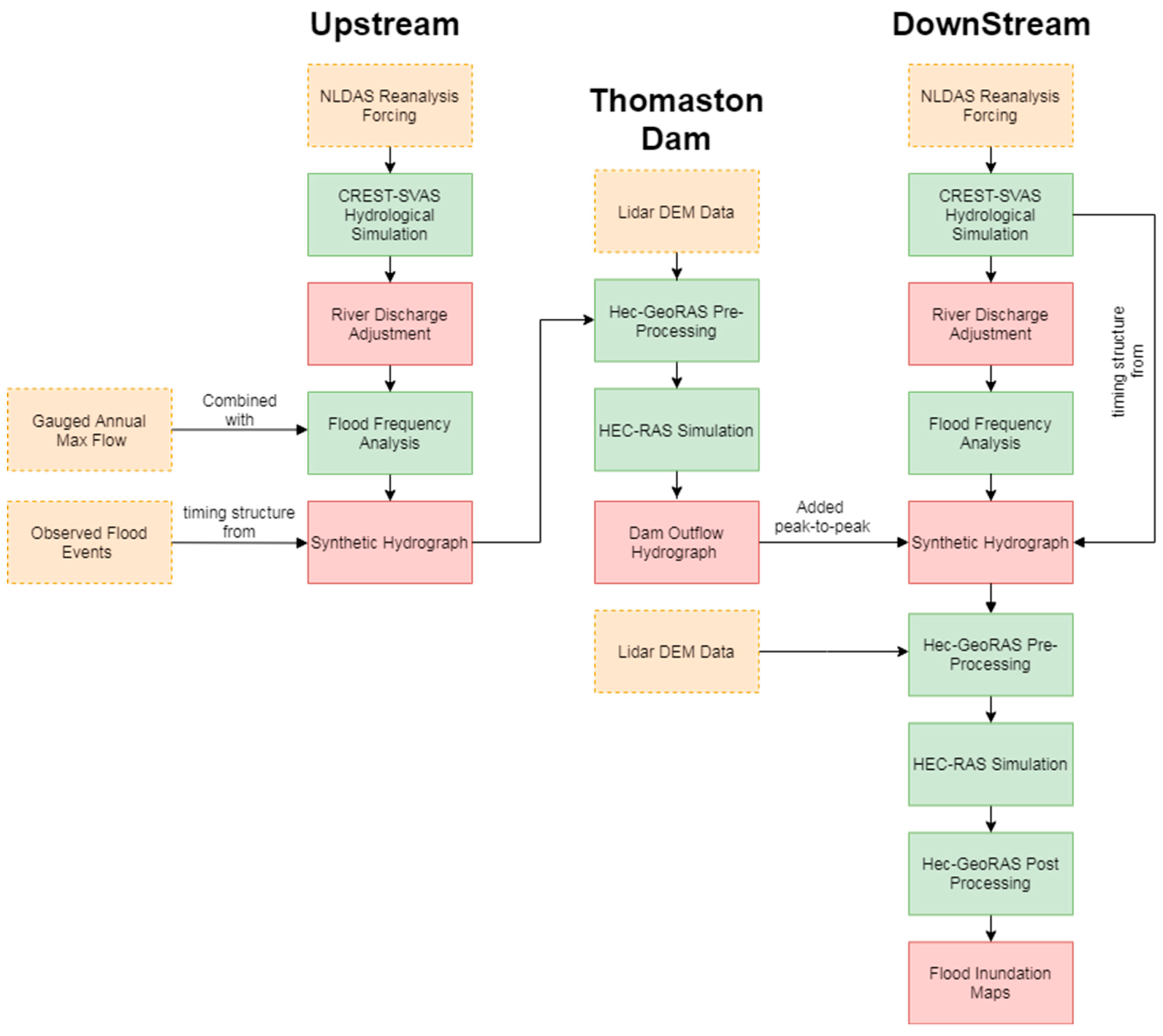
A numerical framework that incorporates high-resolution terrain data, flood frequency analysis (FFA), synthetic events construction, and simulation of dam operation and inundation has been developed within the study (Figure 2). We tested the method in the Naugatuck River of Connecticut. Specifically, peak flows of the Naugatuck River were simulated using the CREST-SVAS model forced with 37-year NLDAS data. Flood frequencies with 0.02, 0.01, 0.005, and 0.002 exceedance probabilities (50, 100, 200, and 500 return year periods, respectively) were estimated by fitting the Log-Pearson Type III distribution. For a given location, the timing structure dictating the shape of flood events was estimated from flood simulation or historical records following a methodology proposed by Archer (2000) [27]. The synthetic hydrograph of flood events of desired return periods was constructed by combining the timing structure and flood magnitude from the FFA. Based on LIDAR-derived high-resolution DEM, these synthetic hydrographs forced HEC-RAS to generate flood inundation maps in a downstream region controlled by a dam.

2.3.1. Hydrological Simulation

This study utilized the newest Coupled Routing and Excess Storage model, version 3.0 with soil–vegetation–atmosphere–snow extension (CREST-SVAS) [13]. CREST-SVAS is a computationally efficient, fully distributed hydrological model designed to simulate flow discharges for large watersheds at a fine spatiotemporal resolution (30 m to 1 km spatial grid resolution and hourly time steps). CREST-SVAS integrates a runoff generation module to simulate vertical fluxes with a routing module to simulate channel discharge at each time step. The runoff generation model couples energy and water balances in four different mediums: atmosphere, canopy, layered snowpack, and soil by solving water and energy balances coupled equations simultaneously. It takes dynamic (precipitation, radiation, humidity, wind speed, leaf area index) and static (land cover, soil properties, impervious ratios) input variables. To best represent the total 37-year timeframe, static maps of land cover and imperviousness from the median year of 2003 were chosen. Due to its strong physical basis and computational efficiency, CREST-SVAS is capable of producing long-term, high-resolution hydrological simulations. Additionally, by physically coupling the snow accumulation/ablation with other water and energy exchanges in the SVA structure, CREST-SVAS gains improved simulation accuracy in situations previously considered difficult mid to high latitude basins with mixed phase precipitation [13]. The mesh size of the hydrological model was 500 m for the land surface simulation while the output variables were resampled to 30-m resolution for routing. In a given flood return period, CREST-SVAS performed hydrological simulations for both the upstream and downstream basins. The flow contribution of the downstream sub-basin is summed with the outflow of the dam, explained later, to calculate the total flow in the downstream area of interest.

2.3.2. Flood Frequency Analysis

Adjustment Technique for Flood Frequency Estimation

As introduced earlier, gridded forcing data of 1/8th-degree (~14 km) spatial resolution is used in this study to force CREST. Our forcing data sacrifices their spatial resolution to obtain relatively high temporal resolution (hourly). Therefore, local extreme precipitation may often be smoothed. Model dependency introduces additional biases. Consequently, it is expected that the simulated flow peak cannot fully capture the reality. In other words, underestimation of flood peaks constantly exists, which in turn, biases the estimation of flood frequency. To address such bias, we applied quantile-based matching technique to post process CREST flow output only to improve the quality of flood frequency estimation. Since the frequency estimation applied here depends solely on maximum annual peak values of the flow time series, only the top-ranked flow rate will affect this estimation. Therefore, we adjust top percentiles values using Equation (1).

$$Q^{obs}\left(p\right)=a{\left[Q^{sim}\left(p\right)\right]}^b, p\ge p_0$$

(1)

where $Q^{obs}\left(p\right)$ and $Q^{sim}\left(p\right)$ stand for observed and simulated flow at p percentile and $p_0$ is the lowest percentile of all annual peaks. Equation (1) is established on the stable relationship of top ranked flow value between observation and simulation.

LPIII Method

Flood frequency analysis is the process of evaluating peak magnitudes and frequencies of past floods to estimate the exceedance probabilities of similar floods. This probability information is vital to the accurate delineation of flood zones and safe design of hydraulic structures [28]. Bulletin #17B of the U.S. Water Resource Council recommends Log-Pearson Type III as the statistical distribution technique to determine peak-flow frequency estimates. Log-Pearson Type III utilizes three statistical parameters: the mean, standard deviation, and skew coefficient to describe the theoretical distribution of the peak-flow data [3]. Flood frequency analysis (LPIII Method) was performed on annual max peaks from the CREST-SVAS simulation in the Naugatuck River basin to generate the necessary flood return period peak flows. The logarithm of simulated annual peak flows was fit following Equation (2):

$$LogQ=\overline{X}+KS$$

(2)

where $\overline{X}$ mean logarithm of annual peak flows and S is the standard deviation of logarithms. K is a factor that depends on the skew coefficient and selected exceedance probability. Values of K can be found in Appendix 3 of Bulletin 17B. The values of $\overline{X}$, S, and skew coefficient were 1.5002, 0.2140, and −0.5098, respectively

2.3.3. Constructing Synthetic Hydrograph

Flood frequency analysis only gives flood peak magnitude information. To credibly model the flood propagation, the hydraulic model requires a complete realistic flood hydrograph rather than assuming a constant flow using the peak value for the entire flood event period.

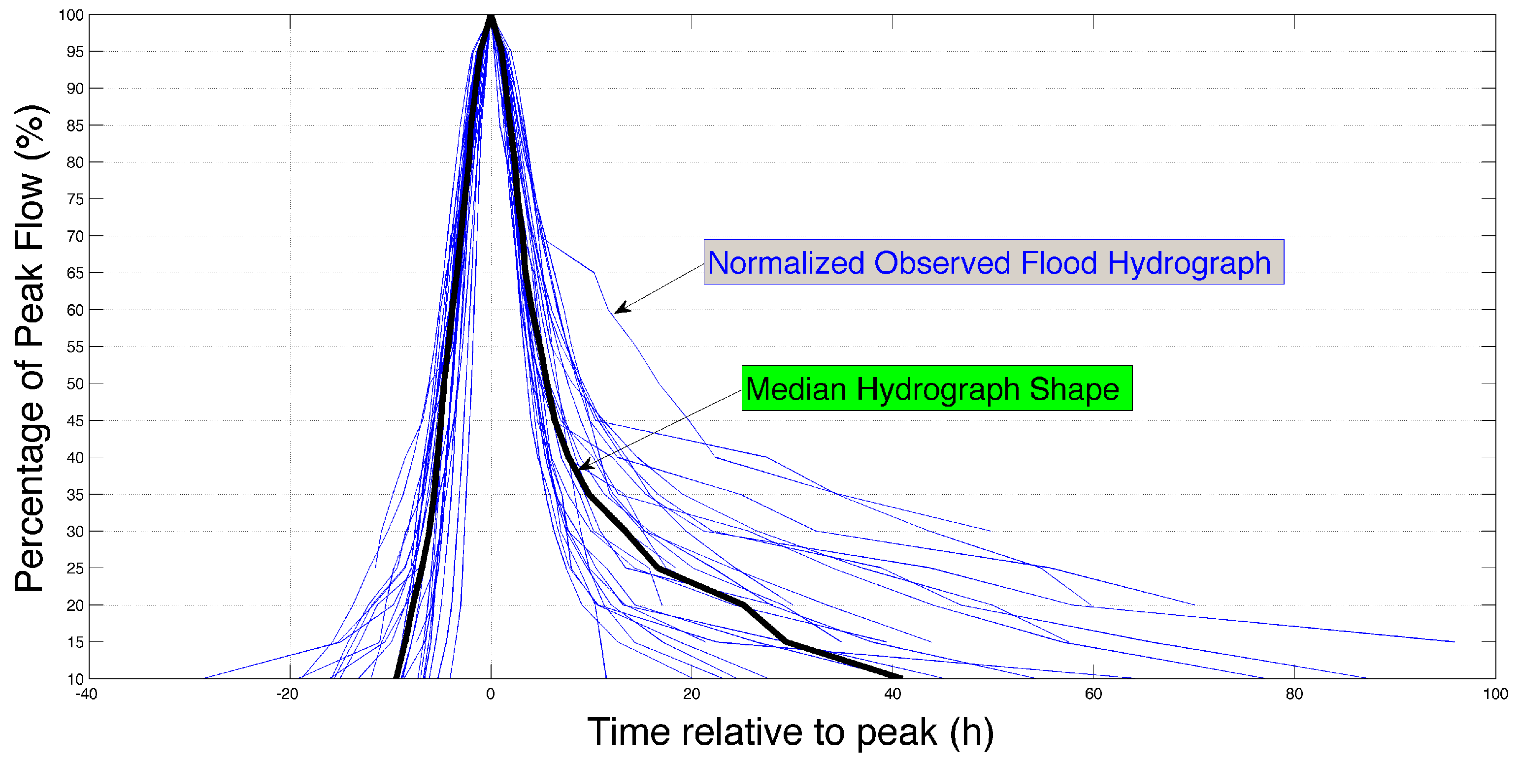
Construction of appropriate synthetic design hydrographs (SDH) is an old topic (e.g., Snyder 1938) that has been revisited over the time by applying several different approaches (Sokolov et al., 1976; Yue et al. 2002; Serinaldi and Grimaldi 2011 among others) [29,30,31,32]. In this work, we adopted a procedure described in Archer et al. (2000), which is, in fact, similar to the typical hydrograph method (Sokolov et al. 1976) but utilizes information from more than just a single hydrograph for the construction of SDH [27]. A similar approach for defining the shape of SDH was also followed by Sauquet et al., (2008) [33]. Archer’s proposed method has the benefit of neither requiring the separation of base flow and storm runoff nor assuming the hydrograph is symmetric, but instead considers the hydrograph in its totality by recreating a normalized median flood hydrograph from observations (Figure 3). The synthetic hydrograph was produced by analyzing only hydrographs corresponding to the highest flow peaks. Specifically, hydrographs with peak flows greater than 100 m³/s (~1-year return period) were considered. This method was used to construct synthetic hydrographs for flood events at 50-, 100-, 200-, and 500-year return periods used as upstream boundary conditions in river reaches “U” and “D”. The same procedure is conducted for both upstream and downstream except that no observation is available for the flow contributed by the downstream part alone. Therefore, the timing structure is retrieved from simulated flow contributed by the downstream drainage area alone. The constructed synthetic hydrographs are finally inputted to HEC-RAS to simulate inundation.

2.3.4. Hydraulic Simulation

To quantify flood risk and identify flood-prone areas, a one-dimensional hydraulic model is used to simulate the spatial distribution of hydraulic variables like water depth and flood inundation extent. Two main forcing factors are required in HEC-RAS: the flood event’s streamflow time-series and bathymetry of the river channel and surrounding floodplain. HEC-RAS is fully compatible with ArcGIS and accepts vector and raster data formats, therefore, the model gains access to one or two-dimensional representations of measured/computed hydraulic parameters at a fine spatial scale. High-resolution topographic data is necessary to capture the finer-scale heterogeneous features of a river and its floodplain and their effects on flood propagation. Airborne LIDAR-based observations provide topography at a finest resolution (1 m) over regional scale. Simulation accuracy is sensitive to DEM resolution. This improvement in resolution directly translates to the model’s ability to accurately map flood inundation extent. Cook et al. (2009) [34] demonstrated that for a given flow and geometric description, HEC-RAS-predicted inundated area decreased by 25% when forced with 6 m LIDAR DEM instead of the 30 m National Hydrographic Dataset (NHD).

In the preprocessing, river cross-sections were extracted from airborne LIDAR-derived. Stream centerlines, river bank lines, predicted flow paths, inline structures, and river and terrain cross-sections were digitized. To accurately capture the meandering river characteristics, cross-section spacing was less than 45 m. These pre-processed river profiles were then exported to HEC-RAS to be used as a basis for one-dimensional hydraulic simulation. Two separate stream sections from the Naugatuck River were modeled and exported to HEC-RAS, one for the upstream section containing the Thomaston Dam (river reach “U”), and the other for the downstream section containing the critical electrical infrastructure (river reach “D”) (Figure 4). Manning’s roughness coefficients were computed from land cover type following Table 3-1 listed in the HEC-RAS 4.1 Reference Manual [35]. Specifically, the Naugatuck river is straight and clean. Thus, a Manning’s “n” value of 0.032 was used for the main open channel. Since the downstream area surrounding the critical infrastructure is highly urbanized and paved, a roughness coefficient of 0.013 was used.

The next step was to incorporate the flood-control dam on the delineated flood plain within HEC-RAS by utilizing the high-resolution topographic data and supplementary building design information (gate characteristics, construction materials, etc.) gathered from correspondence with Thomaston Dam engineers. The Thomaston Dam controlling the upstream reach “U”, is featured by two sluice gates, which are hoisted to limit the flow passing underneath. These gates are 1.73 m wide, can open to a maximum of 3.05 m, and were assigned a typical energy loss coefficient of 0.6. Additionally, this dam is featured by a spillway 4.3 m below the crest to reduce the pressure to the dam and release water in an extreme flooding scenario. In all tested flooding scenarios, flood stages were far below the level to activate the spillway, and, thus, the spillway played no role in downstream inundation and will not be discussed in the scope of this paper.

Multiple plans were simulated in the following flooding scenarios: a 50-year flood event, 100-year flood event, 200-year flood event, and 500-year flood event. In river reach “U”, each simulation was forced by a corresponding synthetic hydrograph with different initial depth conditions and gate operational plans. The plans include fully-open (3.05 m gate openings) and half-open gates (1.525 m gate openings). The conditions include under normal low flow (base flow conditions) and a half-full reservoir. In the first condition, the dam is set to empty when the simulation begins. In the second condition, the reservoir of the dam starts with 50% capacity filled. Water depths and stream velocities were finally output in a total of 16 flooding cases in the upper modeled river reach “U”. The simulated hydrograph’s output from the dam in river reach “U” was then added to the synthetic hydrographs of the same return period for river reach “D”. The hydrographs were added “peak to peak”, where the maxima of upstream hydrograph were combined directly with the maxima of downstream hydrograph with no time delay. This was done to simulate the “worst case scenario” of maximum flooding. The newly altered synthetic hydrographs forced the hydraulic simulation in river reach “D”. Depending on the flood scenario, the outflow from the dam with fully or half-opened gates contributed from 7–20% of the peak streamflow at the outlet of the river reach “D” (

Table 1. Thomaston Dam outflow contribution to downstream basin outlet peak streamflow.

Dam Peak Streamflow Contribution (cms)
Flooding Scenario	Half Open Gates	Fully Open Gates
50 Year
Empty Reservoir	649.3 (9.94%)	704.8 (16.90%)
Half Filled Reservoir	661.7 (11.52%)	732.3 (20.07%)
No Dam	969.4 (66.89%)
100 Year
Empty Reservoir	722.5 (9.20%)	780.4 (15.78%)
Half Filled Reservoir	734.0 (10.52%)	805.7 (18.45%)
No Dam	1088.1 (66.86%)
200 Year
Empty Reservoir	797.6 (8.56%)	857.7 (14.80%)
Half Filled Reservoir	808.4 (9.67%)	881.1 (17.07%)
No Dam	1210.5 (66.83%)
500 Year
Empty Reservoir	900.8 (7.83%)	963.5 (13.68%)
Half Filled Reservoir	910.7 (8.73%)	984.7 (15.52%)
No Dam	1379.2 (66.78%)

), demonstrating the significance of accurate overland runoff simulation from the hydrological model.

Accompanying the 16 cases simulated in river reach “U” two scenarios, closed dam and no dam, were simulated solely in river reach “D”. The closed dam scenario assumes the dam completely congests all upstream contribution, so the hydraulic simulation is forced only by the downstream synthetic hydrograph (thus, having no dam streamflow contribution). The no dam scenario illustrates the potential flooding that would occur if the protection provided by the dam was removed. To simulate this situation, the dam inflow synthetic hydrographs were combined “peak to peak” with the downstream synthetic hydrographs of the same return period. This adds an additional eight flooding cases modeled exclusively in river reach “D”. A table illustrating all of the separate dam operation plans and return periods simulated in river reaches “U” and “D” for this study can be found in

Table 2. Dam operation scenario diagram.

Return Period	Dam Operation	Reservoir Level	Results
50 years	No Dam	N/A	24 FLOOD INUNDATION MAPS
	Closed Dam
	Half Open Gates	Both: Empty and Half Filled
	Fully Open Gates
100 years	No Dam	N/A
	Closed Dam
	Half Open Gates	Both: Empty and Half Filled
	Fully Open Gates
200 years	No Dam	N/A
	Closed Dam
	Half Open Gates	Both: Empty and Half Filled
	Fully Open Gates
500 years	No Dam	N/A
	Closed Dam
	Half Open Gates	Both: Empty and Half Filled
	Fully Open Gates

below.

3. Results

3.1. Validation of Stream Flow Simulations

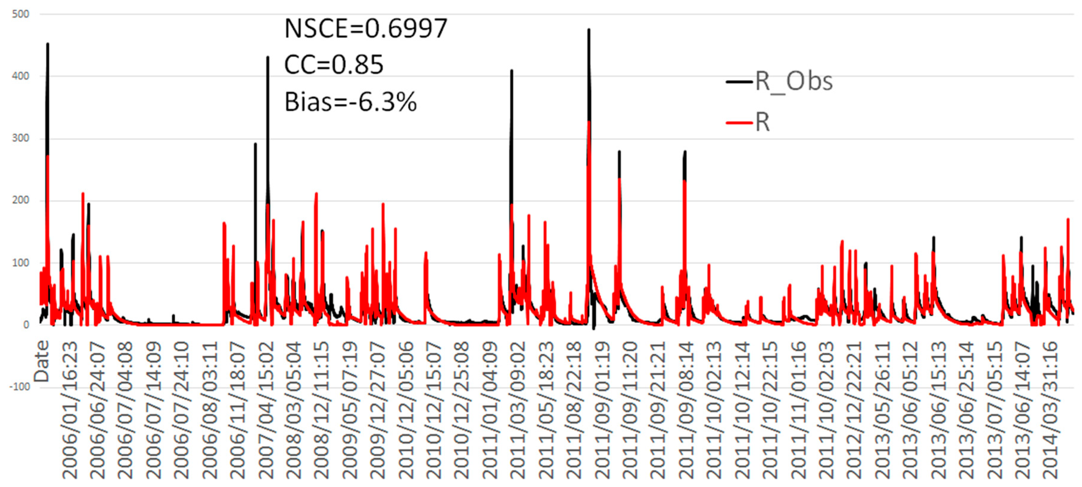
CREST-SVAS hydrologic model simulated streamflows in the watershed upstream of the Thomaston Dam. These streamflows were validated against observed discharges measured by a stream gauge at the inlet of the dam maintained by USACE (U.S. Army Corps of Engineers). A total of 45 events were used for calibration/validation of the model, with nine of the events used for validation. A mosaiced hydrograph of all the events is shown in Figure 5. CREST-SVAS runoff simulations exhibited good agreement with stream flow measurements, with Nash-Sutcliffe coefficient of efficiency (NSCE) [36], Pearson correlation coefficient, and relative bias (see Equations (3)–(5)) being 0.7, 0.85, and −6.3%, respectively.

$$NSCE=1-\frac{{{\displaystyle \sum }}_{t=1}^T{\left(Q_m^t-Q_o^t\right)}^2}{{{\displaystyle \sum }}_{t=1}^T{\left(Q_o^t-\overline{Q_o}\right)}^2}$$

(3)

$Q_o$ is the mean of observed discharges, $Q_m^{}$ is modeled discharge, and $Q_o^t$ is observed discharge at time t. In addition to NSCE, we computed the correlation coefficient and relative bias, defined as:

$$CC=\frac{{{\displaystyle \sum }}_{t=1}^T\left(Q_m^t-\overline{Q_m})(Q_o^t-\overline{Q_o}\right)}{\sqrt{{{\displaystyle \sum }}_{t=1}^T{\left(Q_m^t-\overline{Q_m}\right)}^2}\sqrt{{{\displaystyle \sum }}_{t=1}^T{\left(Q_o^t-\overline{Q_o}\right)}^2}}$$

(4)

$$Bias=\frac{V_m-V_{obs}}{V_{obs}}\times 100$$

(5)

where V_m is the total measured volume and V_obs is the total observed volume.

CREST-SVAS is only calibrated in the sub-basin upstream to the dam. The calibrated routing parameters are applied to both upstream and downstream sub-basins because there is no downstream gauge observation for calibrating these parameters. Please note that CREST-SVAS model uses distributed and physically derived parameters for the simulation of the land surface process (rainfall-direct runoff) and the simulation of the land surface process does not require any calibration. Only the routing parameters that primarily control the time-delay and velocity of flows are needed to be calibrated [13,37].

3.2. Validation of Hydraulic Simulations

Simulated dam outflow from the 27 August 2011, the largest recent flooding event in river reach “U”, were validated against flow rates computed using gate rating curves posted by the U.S. Army Corps of Engineers (see Figure 6). Hydrographs recorded by a stream-gage at the inlet to the dam were used for the model’s upstream boundary condition. The measured flood-control gate height time-series from the Thomaston dam for this same event were used as the operation of the dam in the simulation. During this event, a maximum flood stage of 22.8 m was reached, producing outflow rates of 21.3 cms and 35.2 cms when the gates were half and fully open, respectively. The model displayed good agreement with these two outflow rates, with minor gate discharge discrepancies of only 2.2 cms (10% error) and 4.7 cms (13% error) for the two operational scenarios. 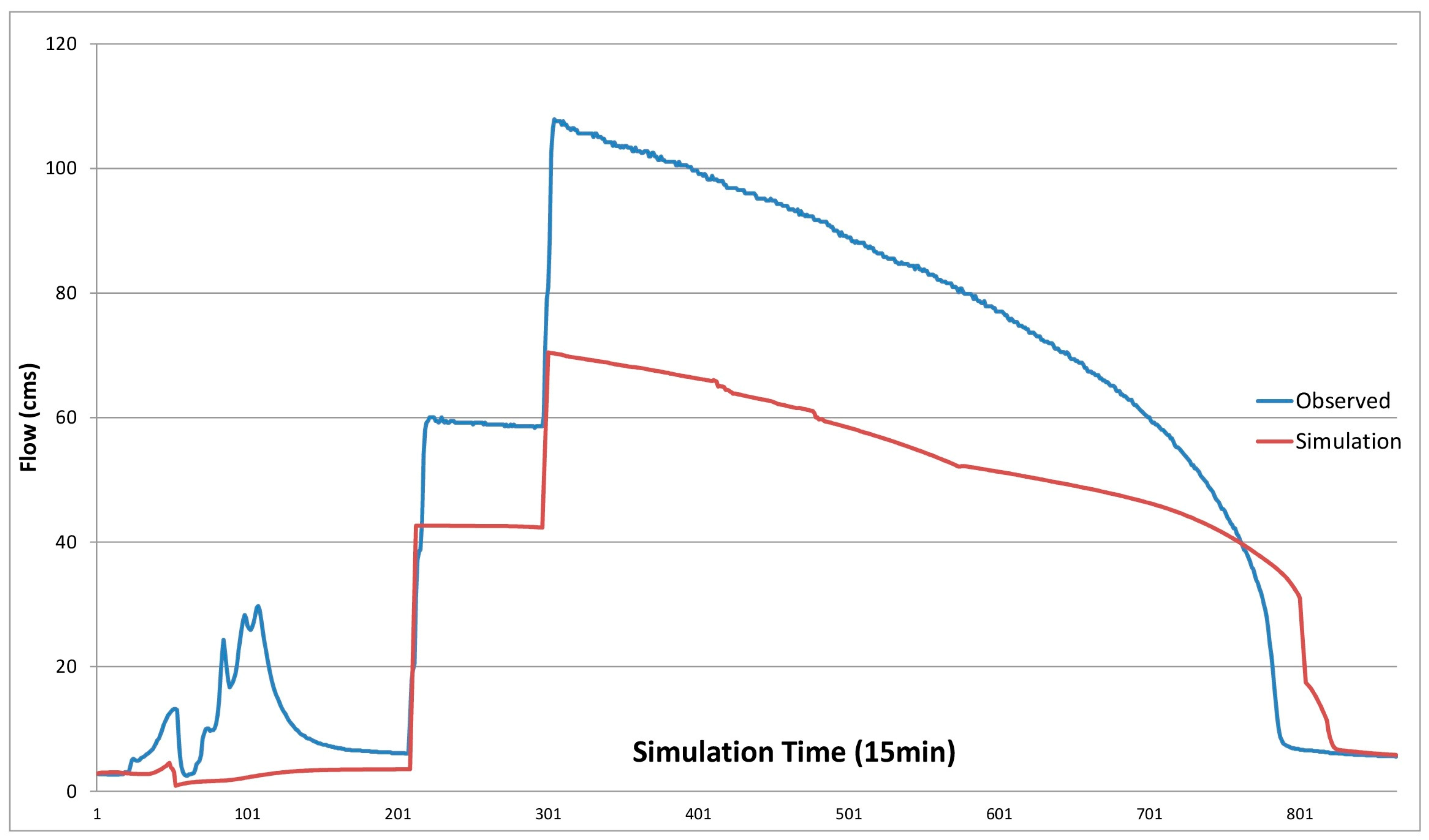Additionally, simulated stream flow rates for the same flooding event in river reach “U” were compared against observed hydrographs from a stream gauge (USGS station 01206900) residing 2.4 km downstream of the Thomaston dam on the Naugatuck River (Figure 7). As seen in the figure, the hydraulic model did well in capturing the overall hydrograph shape; however, it consistently underestimated total streamflow. This underestimation can be explained by overlooking the contributing area between the dam and the USGS gauge location.

4. Discussion

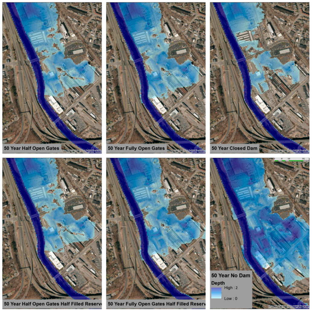
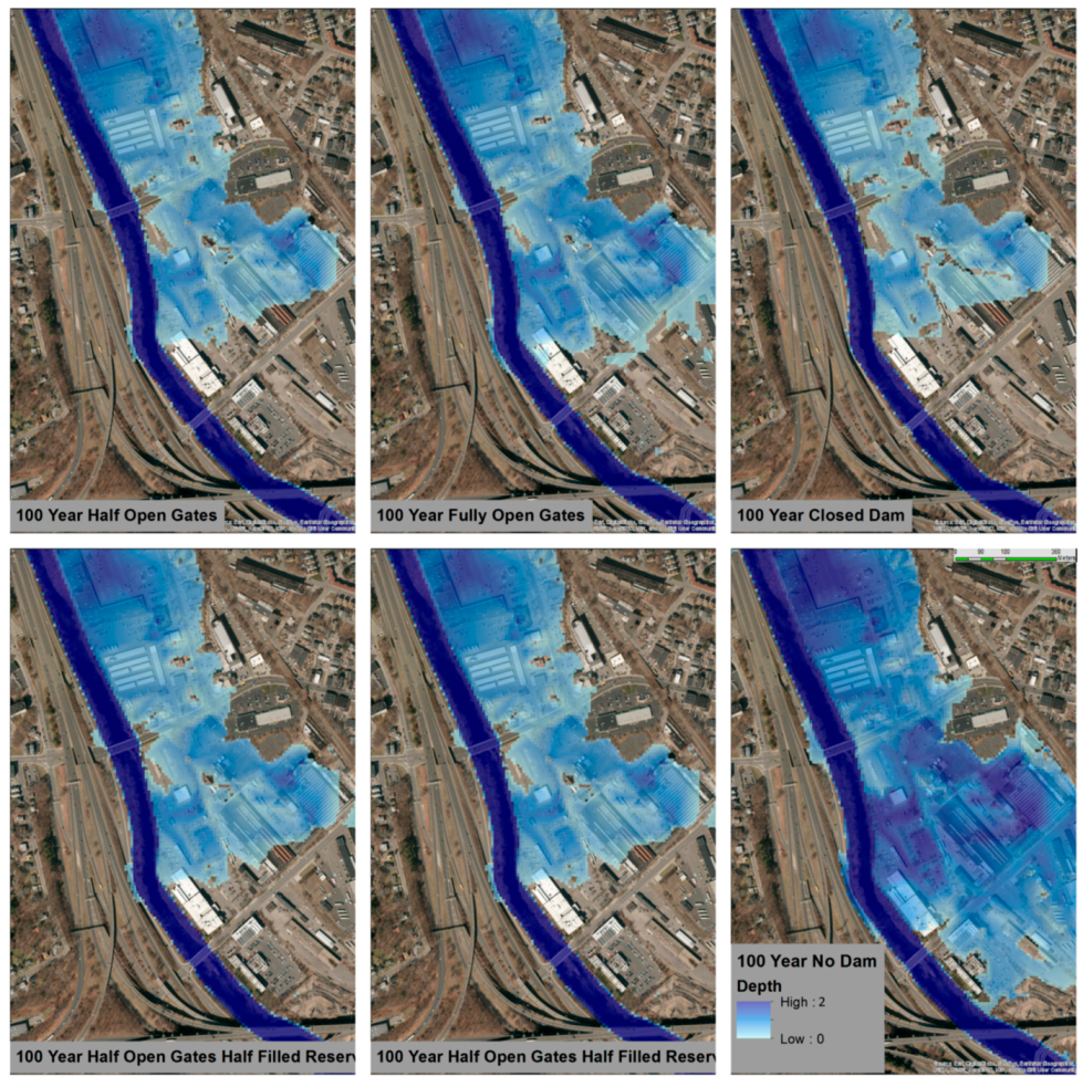
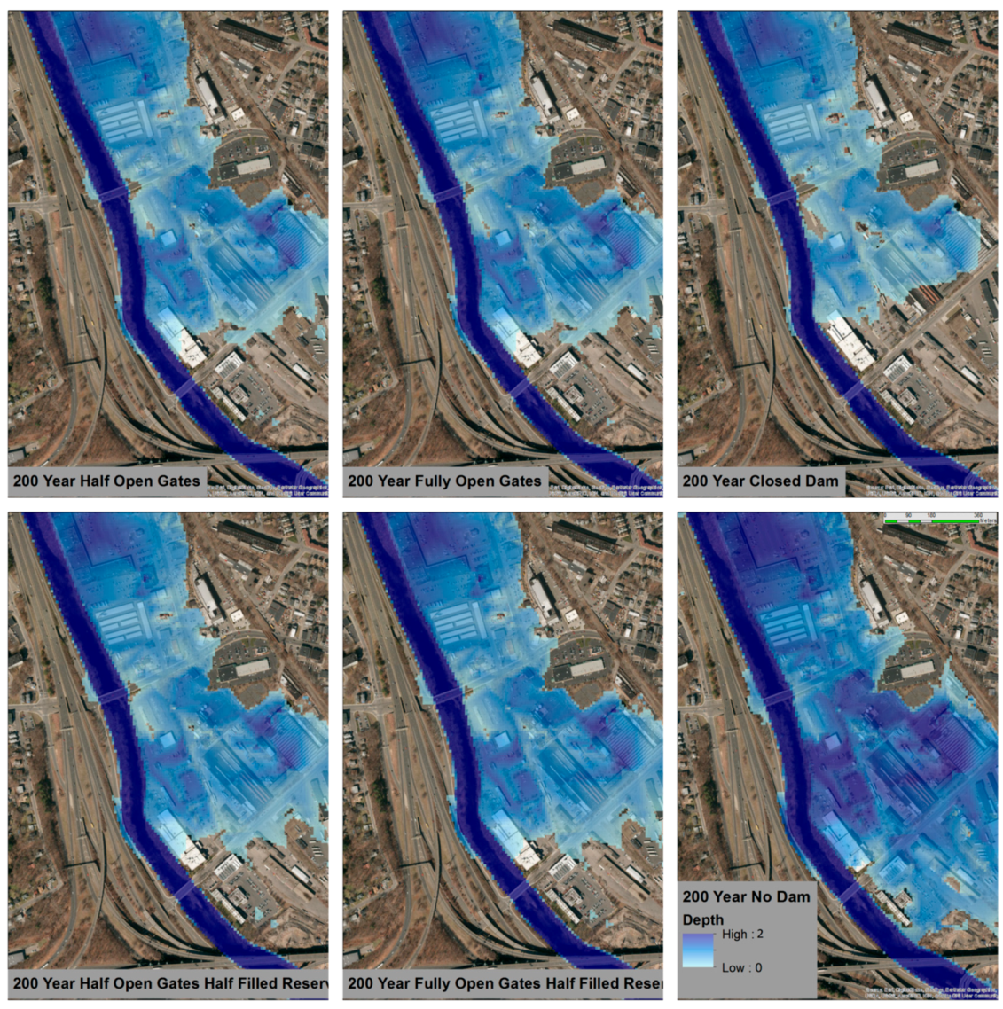
Maximum inundation depth and extent maps simulated by the HEC-RAS model for each of the 24 flooding scenarios in the downstream river reach “D” are illustrated in Figure 8, Figure 9, Figure 10 and Figure 11. Flood extent was determined by subtracting the underlying ground elevation from the LIDAR-derived Triangular irregular networks (TINs) from the water surface profile elevation. If the result was positive, then the area is classified as inundated and assigned a flood depth. Simulated water depths and extents have been co-displayed over satellite imagery to visualize the susceptibility of certain urban areas in Waterbury-CT. A high-end limit of 2 m was utilized in the inundation maps so that the spatial variability of flood depths could be more clearly represented. The majority of flood occurred in the floodplains on the eastern side of the Naugatuck River. An elevated highway that runs along the western edge of the river prevents floods from propagating in that direction.

As shown in the results, a portion of the area of interest, more specifically critical infrastructure “A”, is partially or fully inundated in all flood scenarios. The maximum flood depth in each scenario at critical infrastructure “A” as well as critical infrastructure “B” can be seen in Figure 12. During the “worst case scenario” with the protection of the dam, a 500-year flood with the upstream dam’s reservoir initially half-filled and both flood control gates fully-open, the area of interest experienced an estimated 1.40 and 0.82 m of inundation at critical infrastructure “A” and “B”, respectively. When the dam was removed, these same locations experienced a greatly increased 1.93 (+36.5%) and 1.34 (+79.5%) meters of inundation. However, when the dam was closed, and only the downstream watershed contributed to flooding, critical infrastructure “A” and “B” experienced a decreased 0.82 (−42%) and 0.052 (−94%) meters of flood inundation, respectively. Comparing the no dam and fully-open dam operational scenarios provides direct insight on the role the dam plays in protection by delaying voluminous flood waters from reaching downstream floodplains. Analyzing the closed dam scenario provides an understanding of how upstream streamflow contributes to downstream flood depth, and demonstrates dam’s potential to control inundation, further illuminating the substantial dampening effect the dam has on downstream flood propagation under different dam operational scenarios. The remaining flood return periods (50-year, 100-year, 200-year) experienced similar increases in flood depth when the protection of the dam was removed and decreases in flood depth when the dam was closed. In all scenarios critical infrastructure “A” was more severely affected by flooding than critical infrastructure “B”, likely due to its close proximity to the river’s bank.

This study also examined how different flood infrastructure management strategies impact downstream floodplain areas. The manipulation of the flood control dam’s gate height had a recognizable influence on both estimated maximum flooding extent and flood depth. This influence was more substantial during the 50-year and 100-year higher probability flooding events. With an initially empty dam reservoir, moving from half open to fully open gates produced 165%, 90%, 7%, and 6% increases in maximum water depth at infrastructure A for the 50-, 100-, 200-, and 500-return period simulated extreme flood events. While infrastructure B was dry for the 50- and 100-year flood scenarios, it too saw increases of 33% (200-year) and 21% (500-year) in flood depth when simulated with the same initial empty reservoir conditions.

Comparing the simulated results from model runs with and without an initially filled reservoir illuminates the dam’s ability to dampen the flooding effects in downstream floodplains when hit with a large volume of water from two extreme events in close temporal proximity. During an extreme event, this extra water will likely find its way over the banks and into the downstream floodplain. These results can be seen in Figure 12. Much like the relationship between gate height and maximum water depth and inundation extent, increased effects are found during higher probability, more frequent flood events. When changing from an initially empty reservoir to an initially half-filled reservoir, the model predicted increases in maximum water depth at critical infrastructure “A” of 10% and 63% for a 50-year flood and increases of 24% and 29% for a 100-year flood in maximum water depth at critical infrastructure “A” with gates half and fully-open, respectively. The increases during lower probability extreme events are less severe, resulting in increases of only 6%, 5%, 5%, and 8% (200-year half and fully, 500-year half and fully) maximum water depth at the outside transformer. The initial reservoir stage affected not only water depth but increased the inundation extent, which can be seen in all of the inundation maps.

The results from our study indicated that the existence of the dam served as a major factor in controlling simulated inundation extent and water levels depths downstream. Similar to the trends with gate height and initial water levels in the dam’s reservoir, these effects are more significant in more frequent floods with higher probability (50- and 100-year), increasing maximum simulated water depths at critical infrastructure “A” by 10%, 63%, 24%, and 29% for the 50-year flood return period.

5. Conclusions

Accurate information regarding flood depth and inundation extent are invaluable to the assessment of potential flood risk. In this paper we presented a comprehensive framework for producing flood inundation maps of extreme event scenarios at ungauged locations, and it was demonstrated through a case study at the Naugatuck River in Connecticut. Our methodology links flood frequency analysis with synthetic flow simulations from a physically based, fully distributed hydrologic model, and a one-dimensional hydraulic model. To improve model performance, we utilized long-term atmospheric reanalysis (i.e., NLDAS) to drive ultra-high resolution hydrologic simulations, and a methodology using measured streamflows to create long-return-period flood peak quantiles and synthetic hydrographs at ungauged locations, and fine resolution LIDAR terrain elevation data to construct accurate stream channel profiles.

As a case study, our framework was employed to investigate flood hazard by creating flood inundation maps at the electric utility infrastructure location at the Naugatuck River under four extreme flood events (50-,100-,200-,500-year return period events), two dam operation procedures (gates half- and fully-open), two distinct dam protection setups (closed dam and no dam), and two separate initial dam reservoir conditions (empty reservoir and half-filled reservoir), resulting in a total of 24 flood cases for the electric infrastructure. These inundation maps were combined with satellite imagery to better represent the extent of flooding and potential areas affected.

Our results reveal how the dam assists in improving the resilience of the downstream floodplain. As seen by examining the no dam scenario, the existence of the dam naturally serves to delay flood waters from reaching vulnerable downstream floodplains. Furthermore, by evaluating differing dam gate height and reservoir water level scenarios, we illustrate the ability dam engineers have to further control and delay flood waters from reaching downstream translating directly to reduced maximum flood inundation at downstream critical infrastructure.

We acknowledge that there are potential limitations to the elements of the framework presented. For example, a 2D hydraulic model could potentially offer a better choice to model the flood inundation. However, we should note that the main objective of this paper is to present an integrated framework for flood vulnerability analysis and examine the relative effect of dam operations on the inundation depth values. Therefore, under the assumption that the dynamics (not actual magnitudes) presented between dam operation and flood extent would not change significantly, the choice between 1D vs. 2D model does not affect the main findings of this study. Additionally, Horritt and Bates (2002) [38] pointed out that HEC-RAS at 1D can well predict inundated area. Most recently, Liu et al. (2018) [39] compared HEC-RAS 1D, HEC-RAS 2D, Bristol University’s raster flood inundation model LISFLOOD-FP diffusive, and LISFLOOD-FP subgrid in generating flood inundation extents and concluded that overall, the performance of a 1D model is comparable to the 2D models used in the study, with the 2D models showing slightly better results. Certainly, one could adopt the proposed framework and substitute individual elements (e.g., hydrologic/hydraulic models) based on their own preferences.

Future development of this numerical framework will include, but not limited to integrating novel regional flood frequency analysis (RFFA) approaches that provide more accurate flood frequency estimates by combining flow observation network, satellite-derived flow observation, and high-resolution hydrological simulation, calibrating the hydraulic component using remote sensing retrieved inundation maps, utilizing newly emerging detailed river bathymetric data obtained by penetrating LIDAR and survey, and evaluating the reduction effectiveness of adding low-cost hydraulic infrastructure.