Transient Flow in an Open Channel Bound by Two Step Pumping Stations


Abstract
:1. Introduction
2. Two-Step Pumping Station System
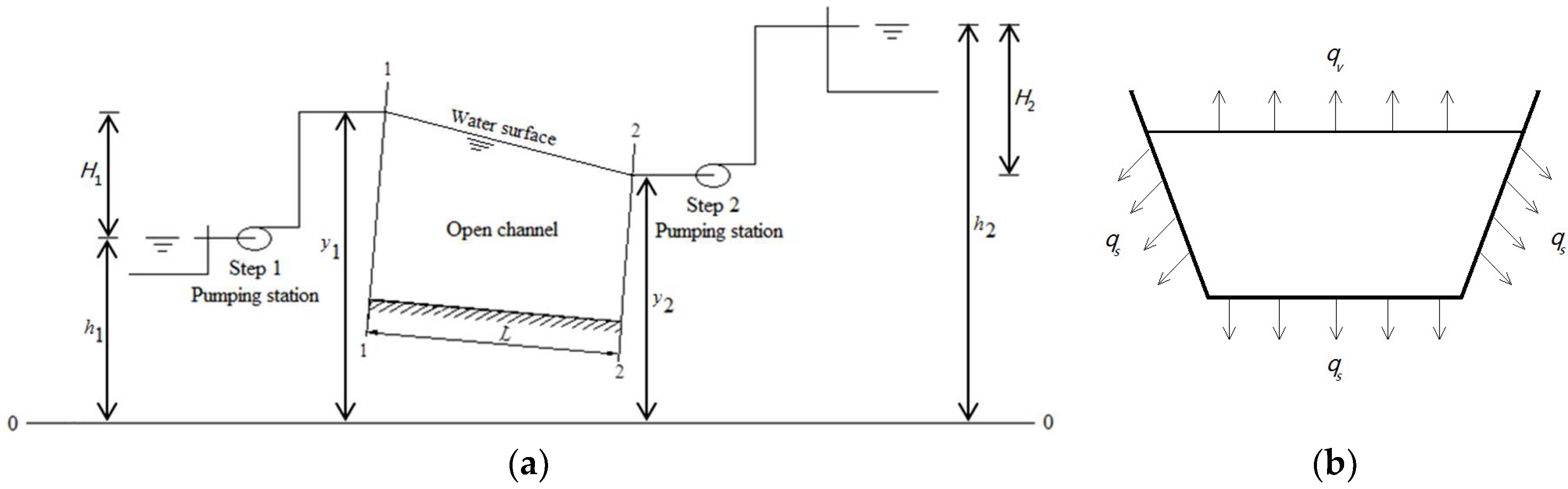
2.1. Definition of Two-Step Pumping Station System
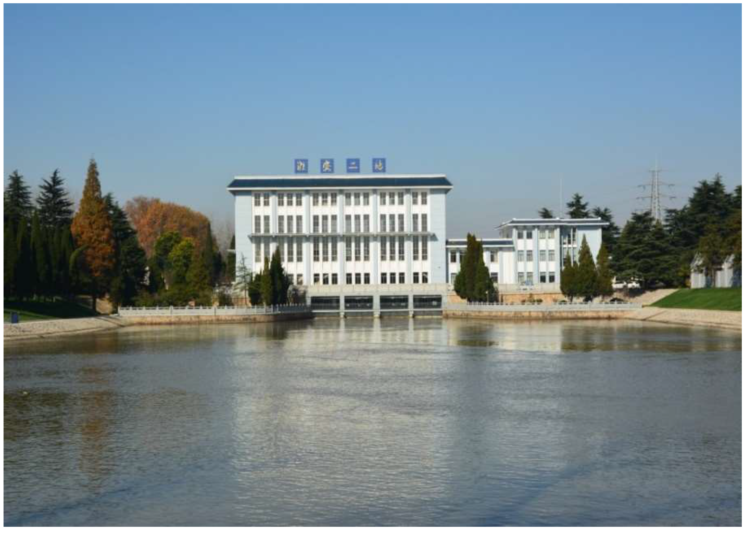
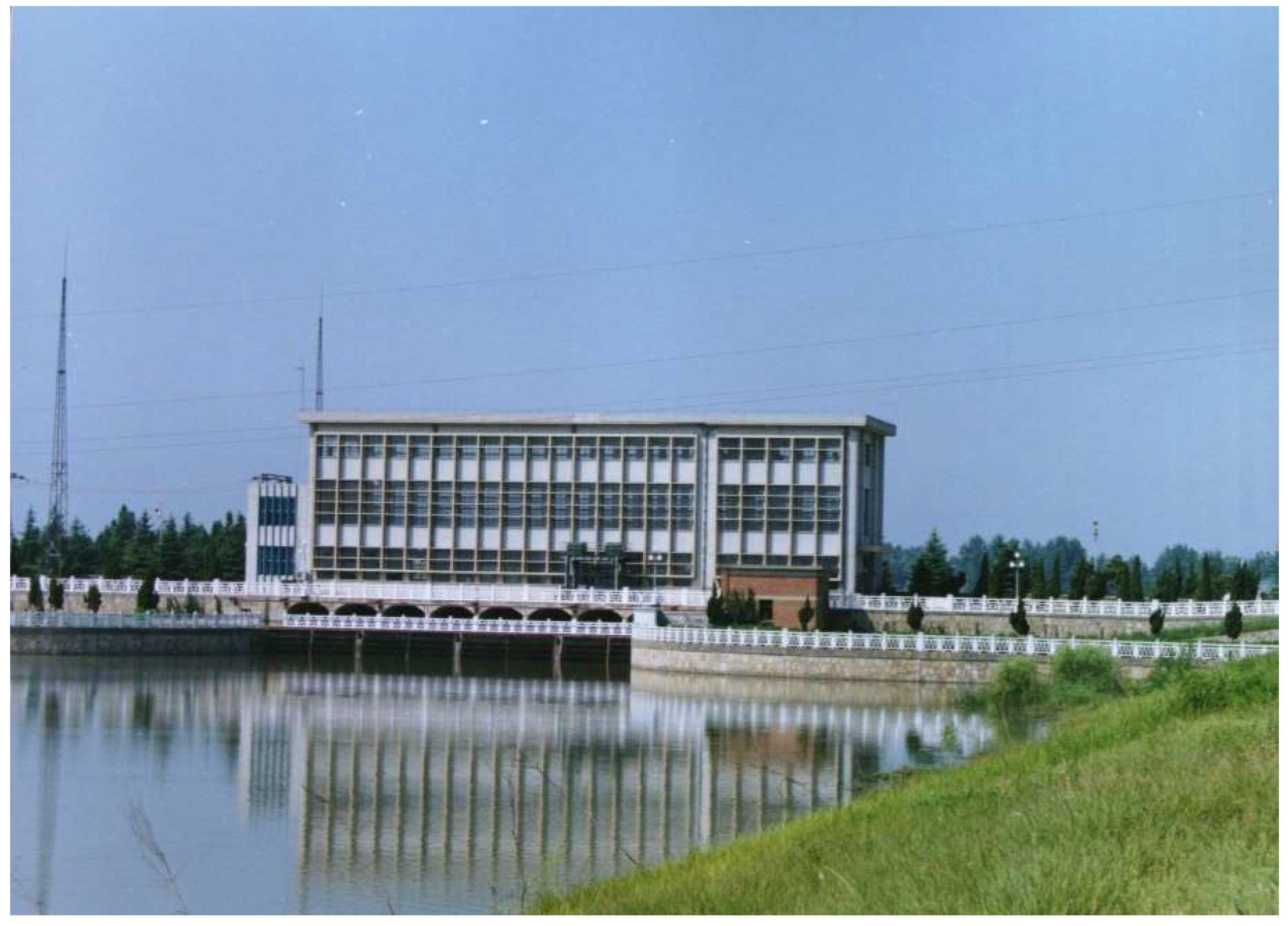
2.2. Background of the Case Study
3. Mathematical Model
3.1. One-Dimensional Open Channel Flow Equations
3.2. Hypotheses of the Saint-Venant Equations
- The flow is one-dimensional, i.e., the velocity is uniform over the cross-sectional area, and the water level across the section is horizontal.
- The streamline curvature is small and vertical accelerations are negligible; hence, the pressure is hydrostatic.
- The effects of boundary friction and turbulence can be accounted for through resistance laws analogous to those used for steady-state flow.
- The average channel bed slope is small so that the cosine of the angle it makes with the horizontal may be replaced by unity.
- The variation of the channel width along x is small.
3.3. Boundary Conditions
3.4. Initial Conditions
4. Finite Difference Method
4.1. Lax Diffusive Scheme
4.2. Stability Conditions
5. Case Study
6. Results and Discussion
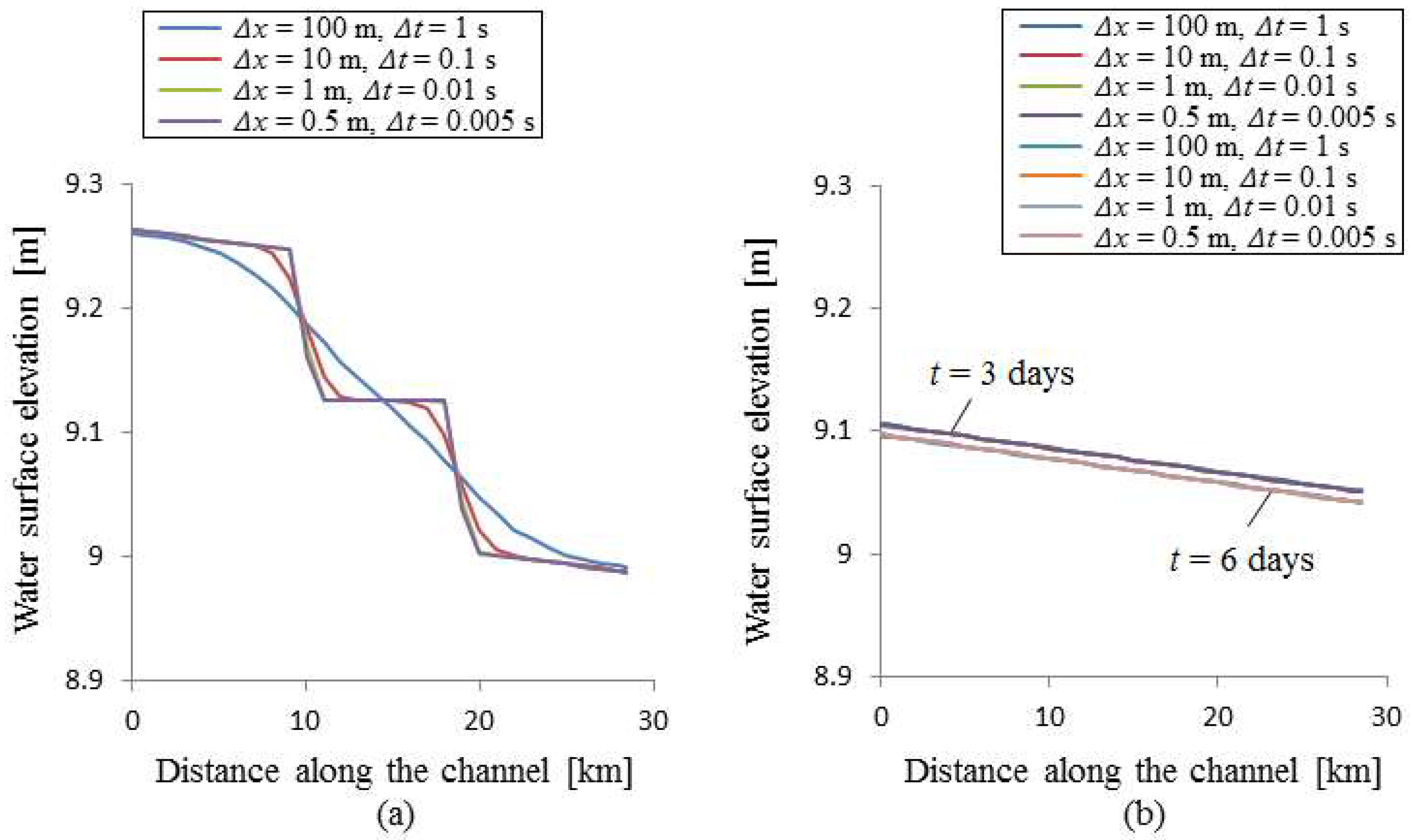
6.1. Grid Size, Accuracy and Computational Time
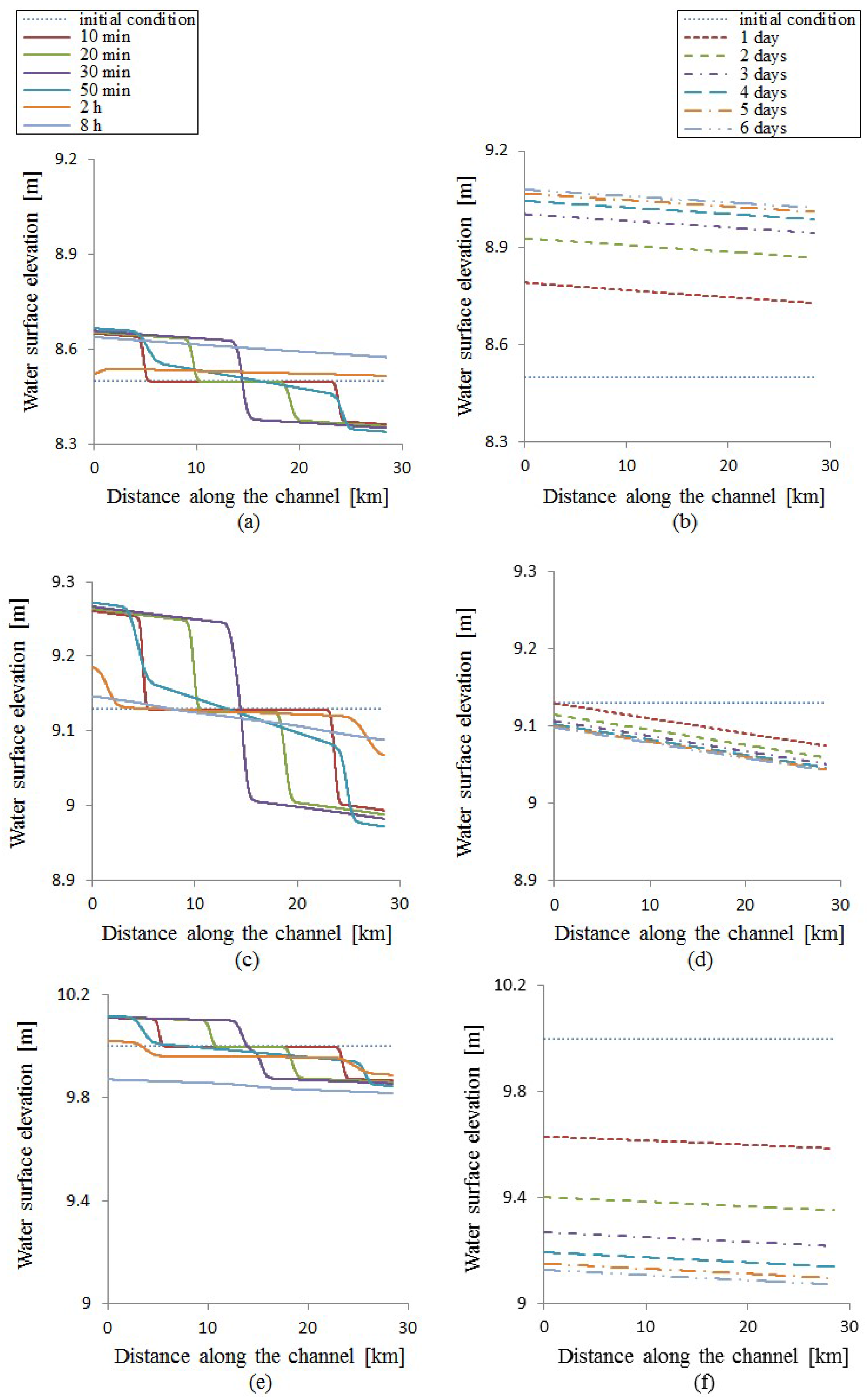
6.2. Water Surface Elevation Along the Channel
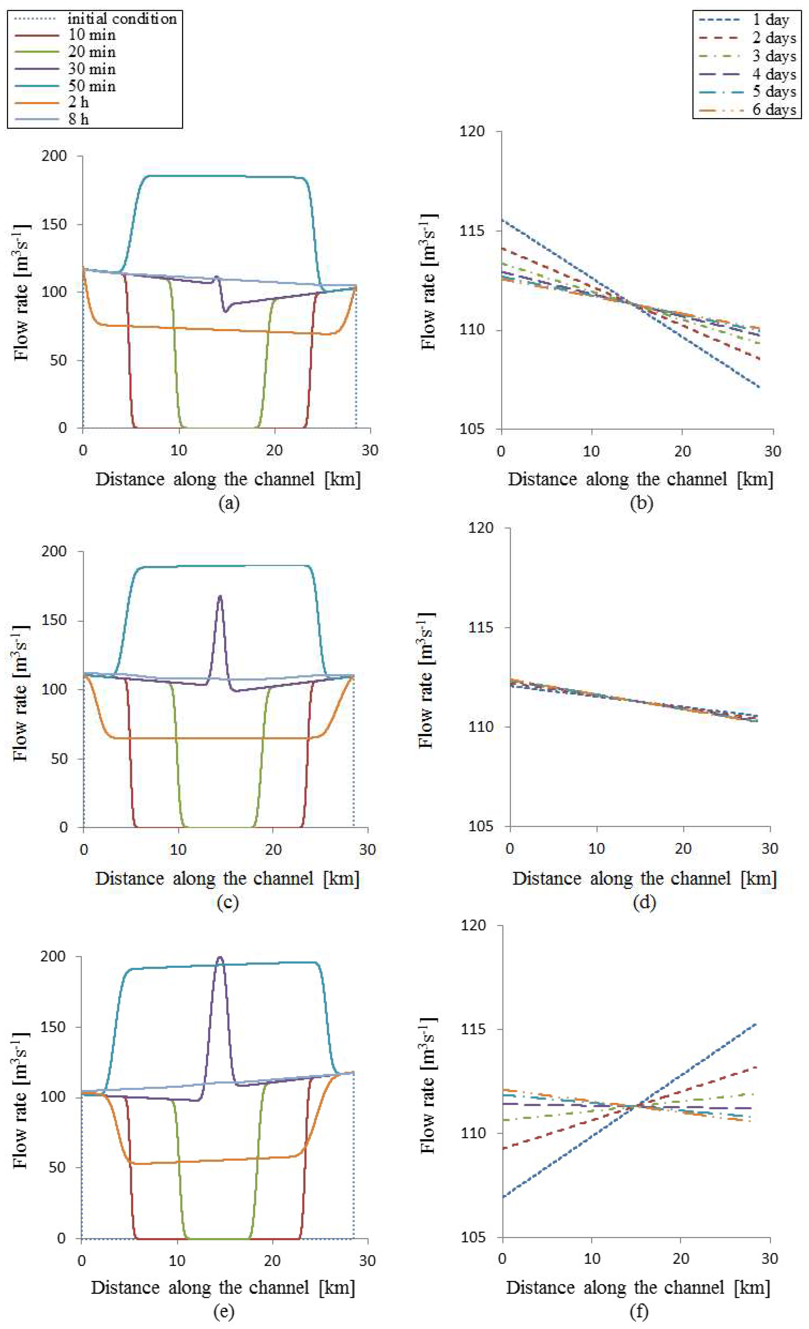
6.3. Flow Rate Along the Channel
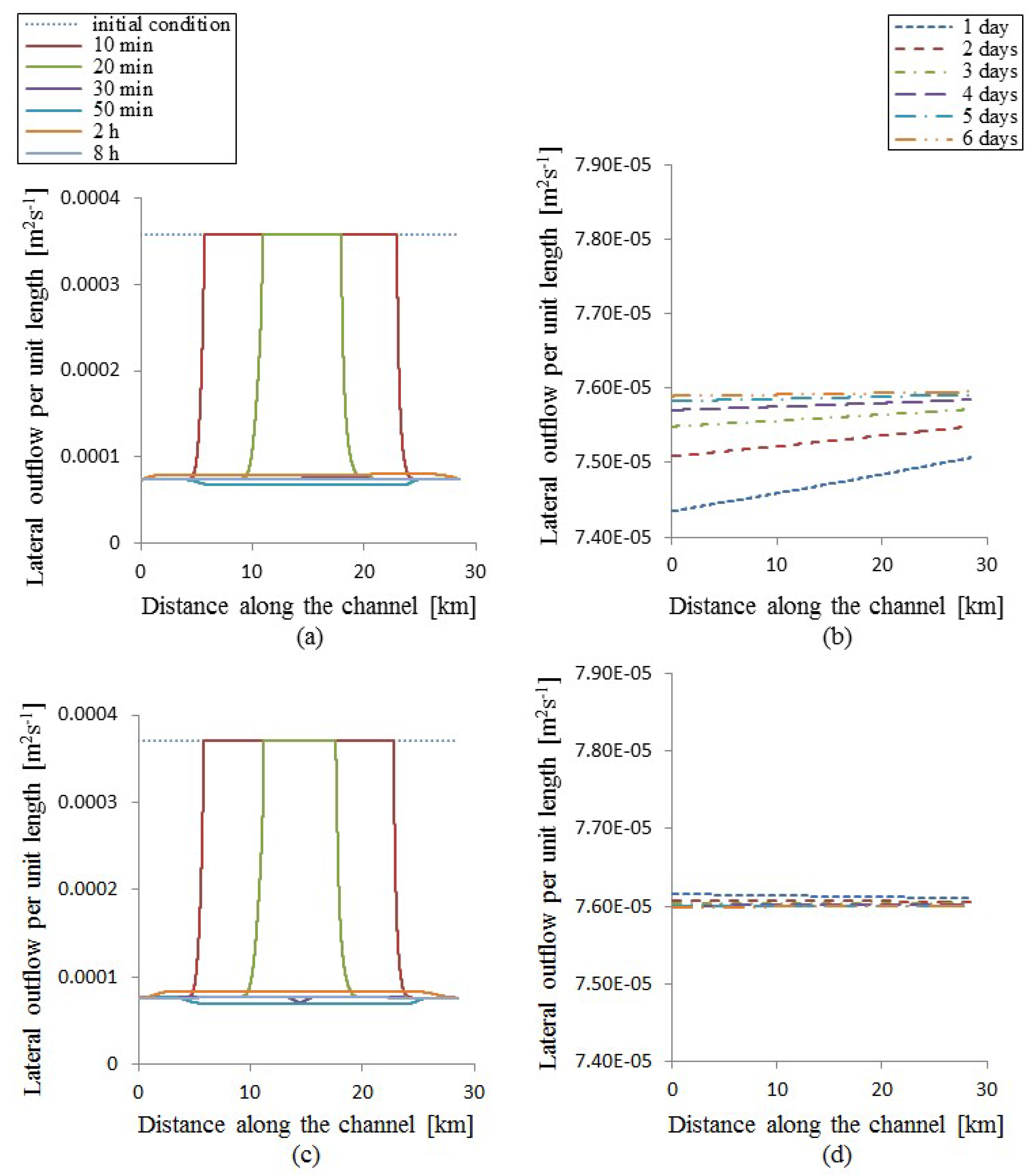
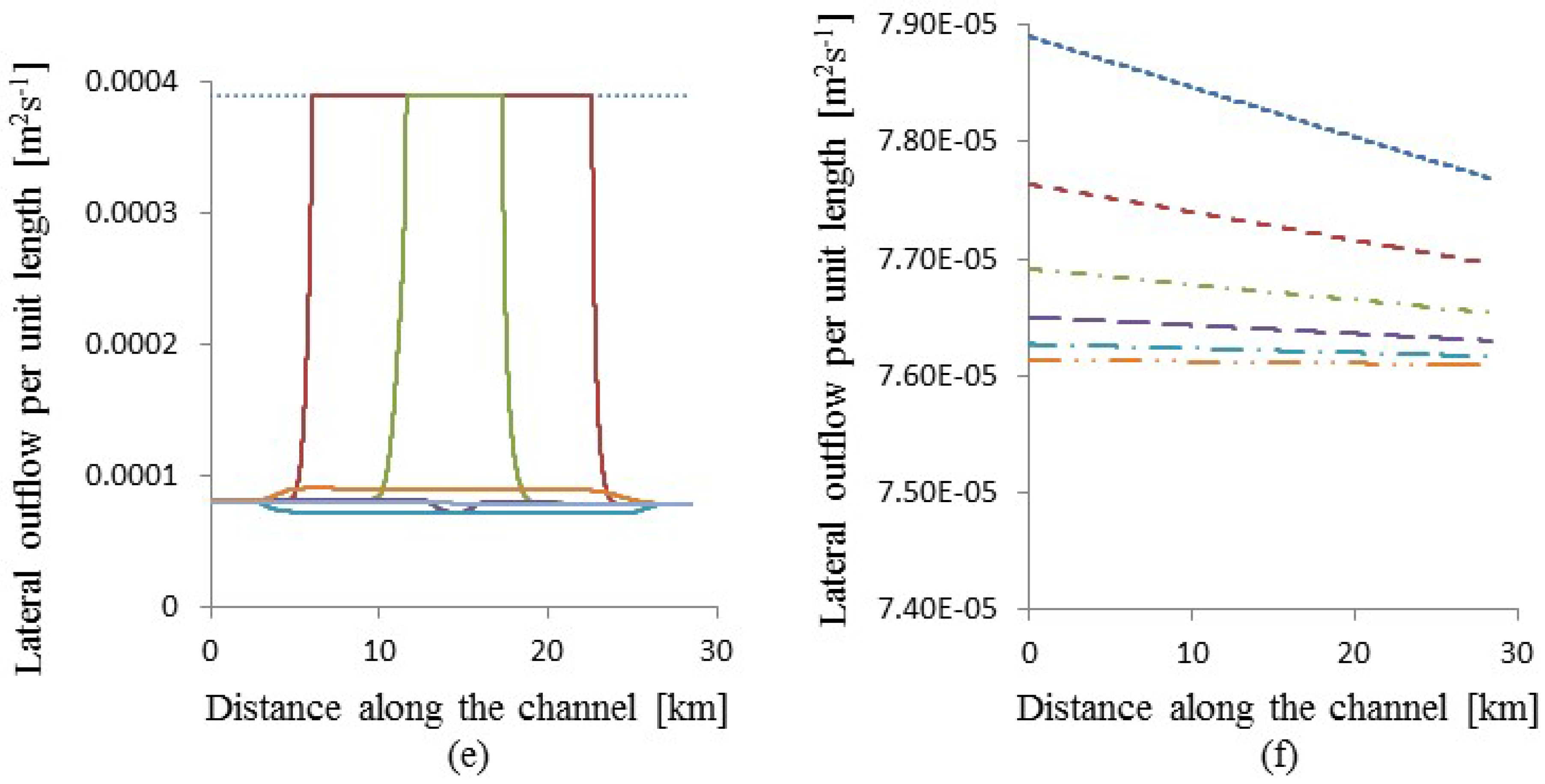
6.4. Lateral Outflow per Unit Length Along the Channel
6.5. Transient Flow Formation Mechanism (Wave Propagation Mechanism)
7. Conclusions
- (1)
- The accuracy of the model was calculated by varying the scheme grid steps. In order to guarantee the stability and the computational accuracy at all times, the optimal distance step obtained was Δx = 1 m, while the optimal time step was Δt = 0.01 s.
- (2)
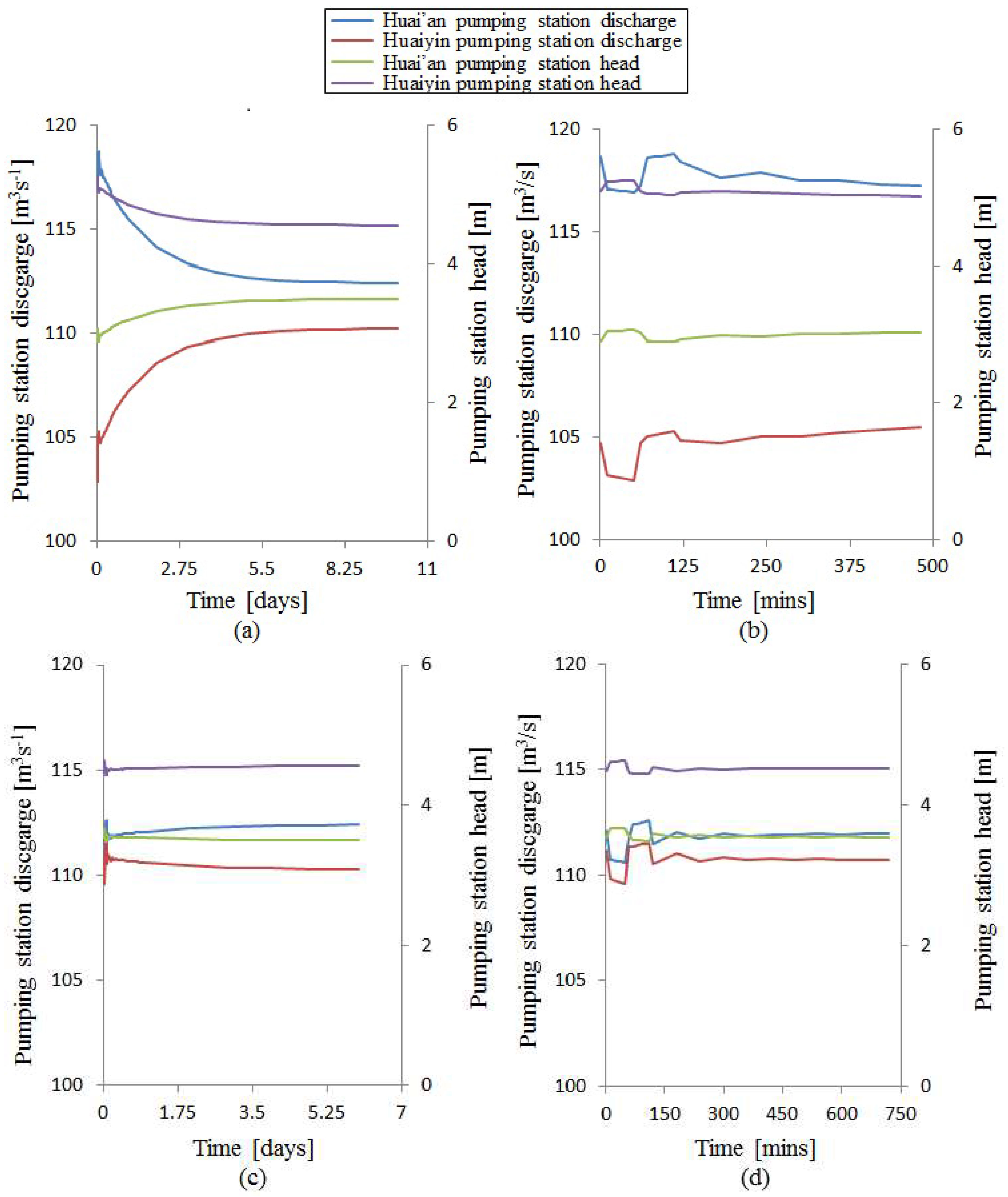
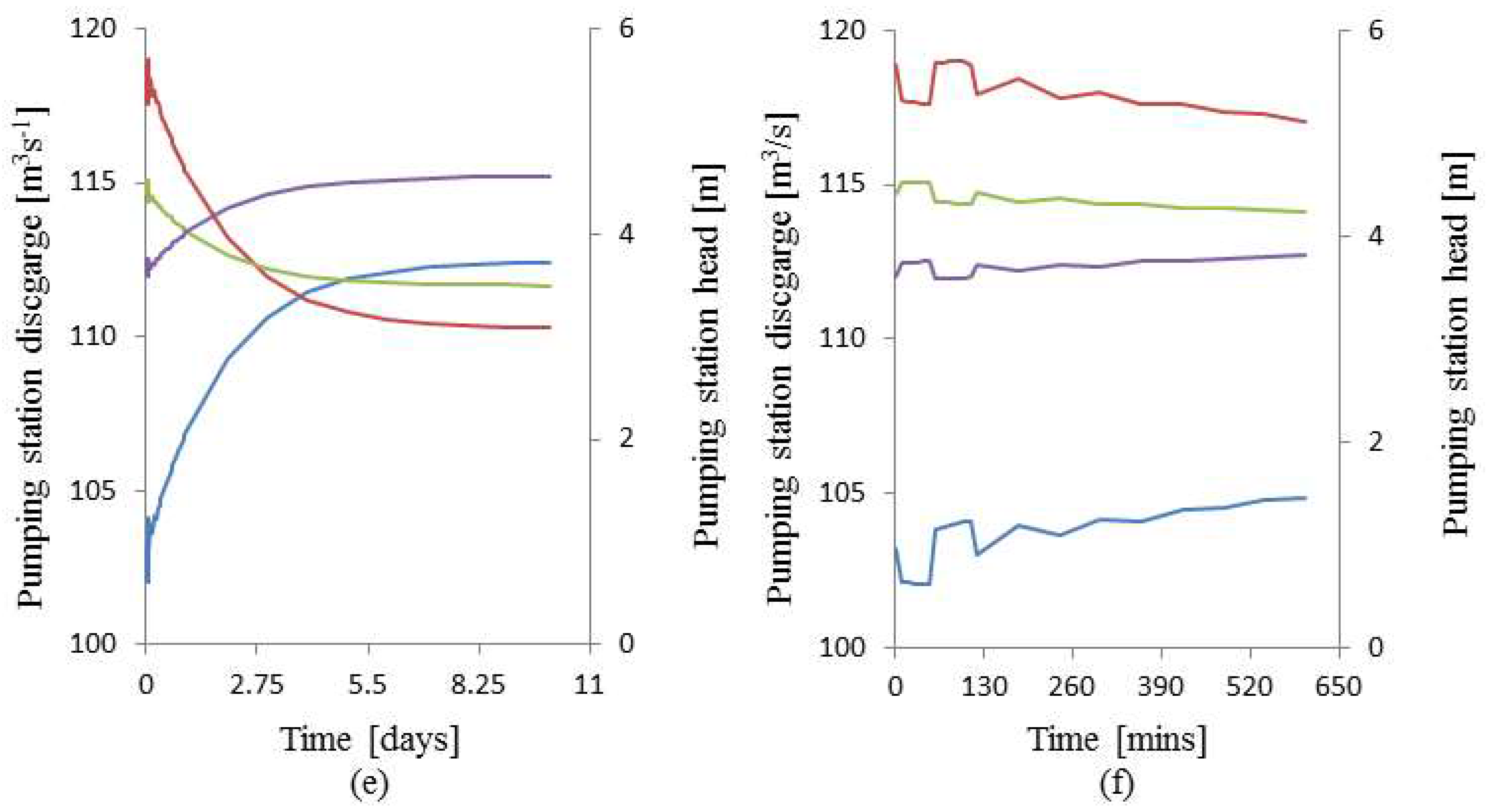
- We calculated and discussed the water surface elevation, the flow rate and the lateral outflow per unit length at various times along the channel. In Huai’an pumping station (upstream), the last water level value was 9.096 m, and the pumping station’s discharge was 112.4 m3 s−1 with a head of 3.496 m. In contrast, in Huaiyin pumping station (downstream), the last water level value was 9.040 m, and the pumping station’s discharge was 110.3 m3 s−1 with a head of 4.560 m. The lateral outflow along the channel was 2.164 m3 s−1.
- (3)
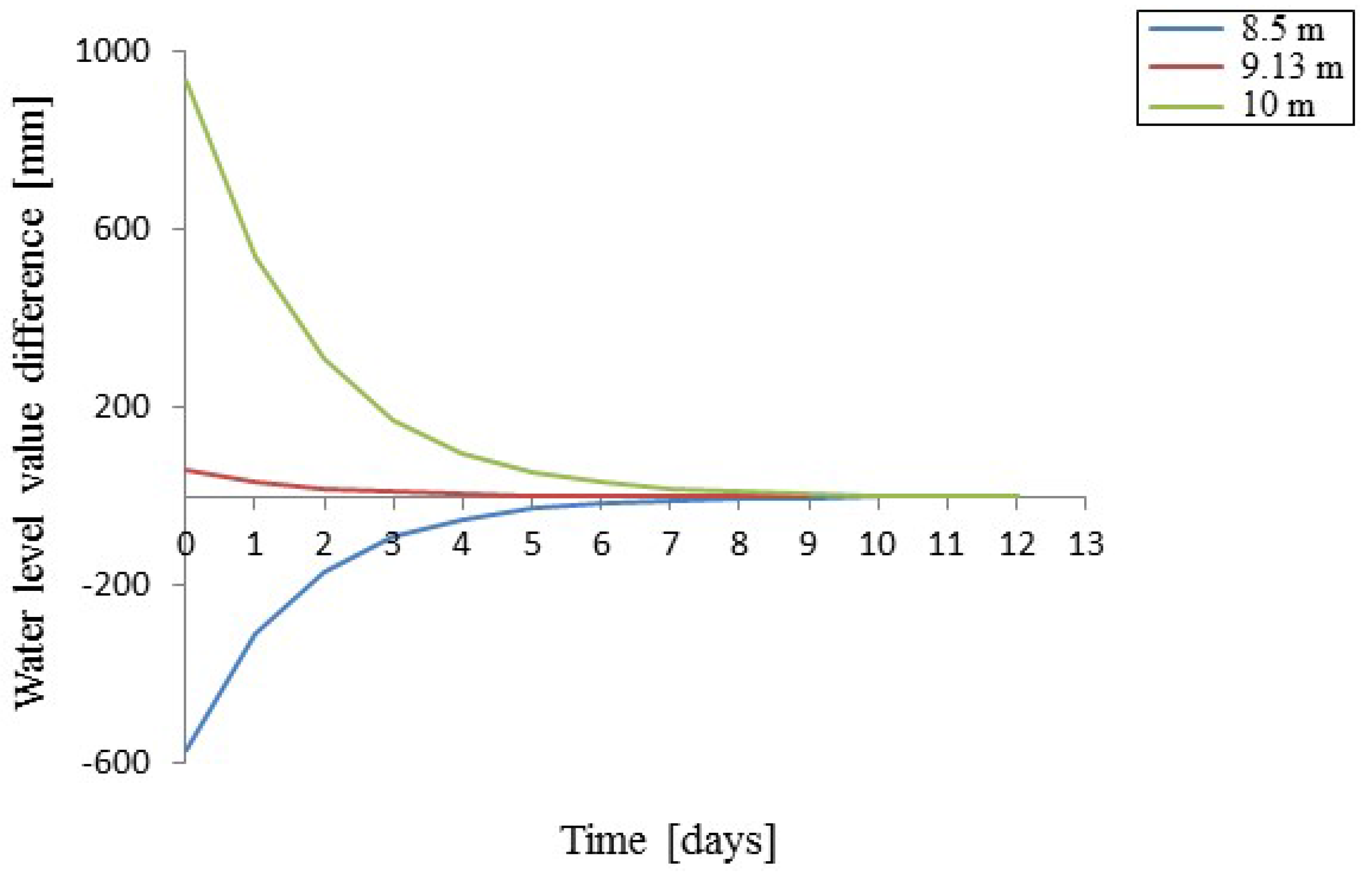
- The computed results showed that the water surface profile, the flow rate and the lateral outflow along the channel are influenced by the initial water level value at which the unsteady flow occurs. Different initial water levels tend towards the same results in terms of water surface profile and flow rate. The time required to reach the almost steady state after the transient produced in the open channel also depends on the initial water level value.
- (4)
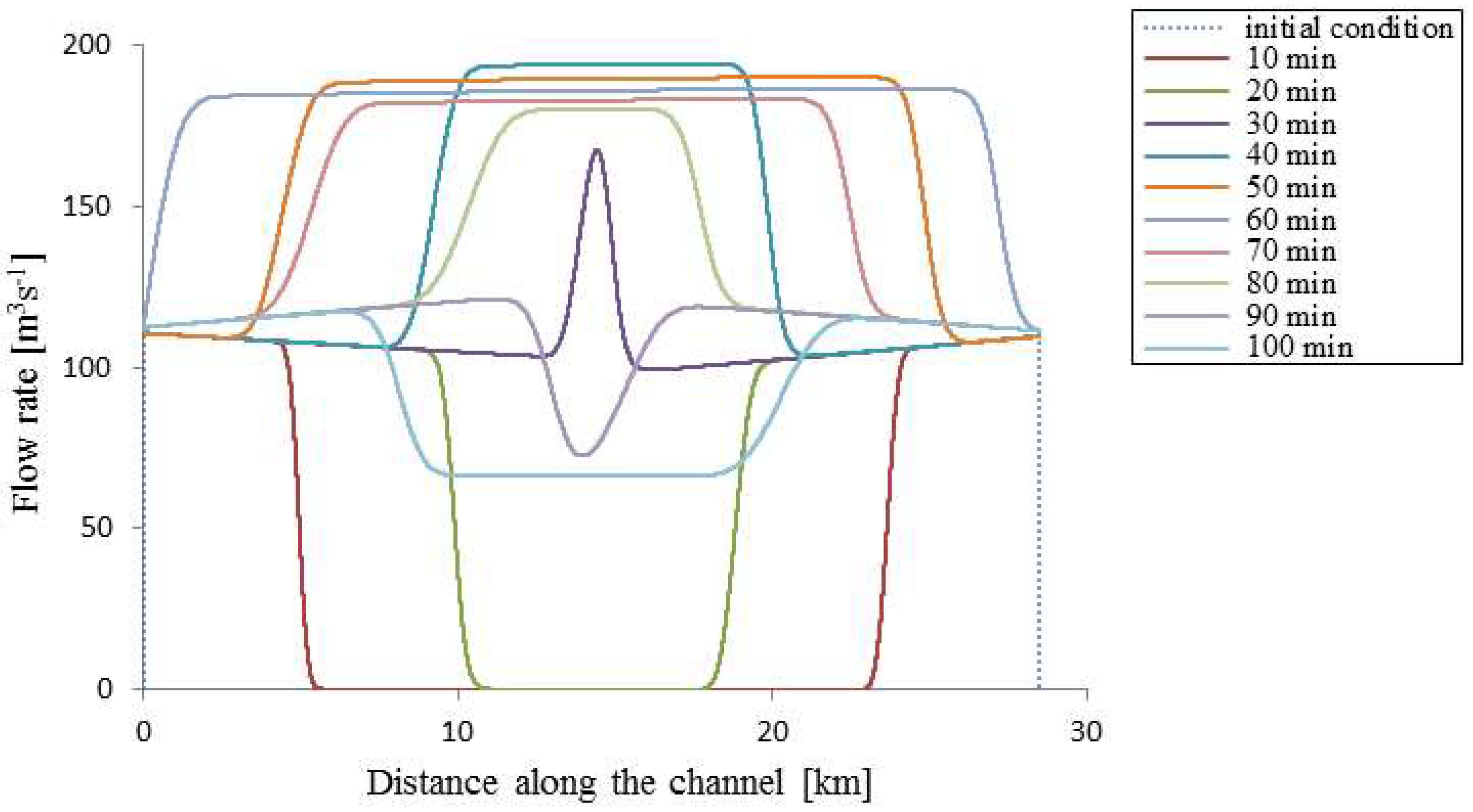
- The wave propagation mechanism is clearly presented and analyzed. Interestingly, two waves were generated. A positive wave moves in the flow direction, whereas a negative wave moves in the opposite direction. Over time, these two waves meet each other near the middle of the channel, thereby increasing the water surface slope. As a result, the flow rate rises in this area and generates two waves that travel in opposite directions to the channel ends. Afterwards, the waves reflect back to the middle of the channel to meet each other again, but in this process, the flow rate decreases gradually from the two ends to the middle of the channel. Then, the two waves travel in opposite directions to the channel ends. Subsequently, they reflect back to the middle of the channel to meet each other again, and the process repeats itself. The amplitudes of these two waves when they meet each other become increasingly small until the steady state is reached.
- (5)
- The accuracy of the results was assessed by comparing the computed results with measured data.
- (1)
- We will study the transient flow in an open channel between two step pumping stations under abnormal situations, such as when one pumping station cannot start up, or when one pump unit breaks down suddenly.
- (2)
- We will study the transient flow for a system with three and more step pumping stations.
- (3)
- We will study the optimal operation of a step pumping station system.
Acknowledgments
Author Contributions
Conflicts of Interest
References
- Te Chow, V. Open Channel Hydraulics; McGraw-Hill Book Company, Inc.: New York, NY, USA, 1959. [Google Scholar]
- Akan, A.O. Open Channel Hydraulics; Butterworth-Heinemann: Oxford, UK, 2011. [Google Scholar]
- Cunge, J.A.; Holly, F.M.; Verwey, A. Practical Aspects of Computational River Hydraulics; Pitman Publishing Ltd.: London, UK, 1980. [Google Scholar]
- Chaudhry, M.H. Open-Channel Flow; Springer Science & Business Media: Berlin, Germany, 2007. [Google Scholar]
- Battjes, J.A.; Labeur, R.J. Unsteady Flow in Open Channels; Cambridge University Press: Cambridge, UK, 2017. [Google Scholar]
- Amein, M.; Chu, H.-L. Implict numerical modeling of unsteady flows. J. Hydraul. Div. 1975, 101, 717–731. [Google Scholar]
- Rahimpour, M.; Tavakoli, A. Multi-grid beam and warming scheme for the simulation of unsteady flow in an open channel. Water SA 2011, 37, 229–235. [Google Scholar] [CrossRef]
- Souza, R.O.D.; Chagas, P. Solution of saint venant’s equation to study flood in rivers, through numerical methods. Hydrol. Days 2005, 2005, 205–210. [Google Scholar]
- Ojiambo, V.; Kinyanjui, M.; Theuri, D.; Kiogora, P.; Giterere, K. A mathematical model of the fluid flow in circular cross-sectional open channels. Certif. Int. J. Eng. Sci. Innov. Technol. (IJESIT) 2014, 3, 335–343. [Google Scholar]
- Kamboh, S.A.; bt Sarbini, I.N.; Labadin, J. Simulation of 2d surface flow in open channel using explicit finite difference method. In Proceedings of the 9th International Conference on IT in Asia (CITA), Kuching, Malaysia, 4–5 August 2015. [Google Scholar]
- Shang, Y.; Liu, R.; Li, T.; Zhang, C.; Wang, G. Transient flow control for an artificial open channel based on finite difference method. Sci. China Technol. Sci. 2011, 54, 781–792. [Google Scholar] [CrossRef]
- Szymkiewicz, R. Finite-element method for the solution of the saint venant equations in an open channel network. J. Hydrol. 1991, 122, 275–287. [Google Scholar] [CrossRef]
- Tavakoli, A.; Zarmehi, F. Adaptive finite element methods for solving saint-venant equations. Sci. Iran. 2011, 18, 1321–1326. [Google Scholar] [CrossRef]
- Zarmehi, F.; Tavakoli, A.; Rahimpour, M. On numerical stabilization in the solution of saint-venant equations using the finite element method. Comput. Math. Appl. 2011, 62, 1957–1968. [Google Scholar] [CrossRef]
- Audusse, E.; Bristeau, M.-O. Finite-volume solvers for a multilayer saint-venant system. Int. J. Appl. Math. Comput. Sci. 2007, 17, 311–320. [Google Scholar] [CrossRef]
- Ding, Y.; Liu, Y.; Liu, X.; Chen, R.; Shao, S. Applications of coupled explicit–implicit solution of SWEs for unsteady flow in Yangtze River. Water 2017, 9, 91. [Google Scholar] [CrossRef]
- Aricò, C.; Nasello, C. Comparative analyses between the zero-inertia and fully dynamic models of the shallow water equations for unsteady overland flow propagation. Water 2018, 10, 44. [Google Scholar] [CrossRef]
- Akbari, G.; Firoozi, B. Implicit and explicit numerical solution of saint-venant’s equations for simulating flood wave in natural rivers. In Proceedings of the 5th National Congress on Civil Engineering, Mashhad, Iran, 4–6 May 2010. [Google Scholar]
- Machalinska-Murawska, J.; Szydłowski, M. Lax-wendroff and mccormack schemes for numerical simulation of unsteady gradually and rapidly varied open channel flow. Arch. Hydro-Eng. Environ. Mech. 2014, 60, 51–62. [Google Scholar] [CrossRef]
- Viero, D.P.; Peruzzo, P.; Defina, A. Positive surge propagation in sloping channels. Water 2017, 9, 518. [Google Scholar] [CrossRef]
- Gu, S.; Zheng, X.; Ren, L.; Xie, H.; Huang, Y.; Wei, J.; Shao, S. SWE-sphysics simulation of dam break flows at south-gate gorges reservoir. Water 2017, 9, 387. [Google Scholar] [CrossRef]
- Liu, H.; Wang, H.; Liu, S.; Hu, C.; Ding, Y.; Zhang, J. Lattice boltzmann method for the saint–venant equations. J. Hydrol. 2015, 524, 411–416. [Google Scholar] [CrossRef]
- Chun, S.; Merkley, G. ODE solution to the characteristic form of the saint-venant equations. Irrig. Sci. 2008, 26, 213–222. [Google Scholar] [CrossRef]
- Ferreira, D.M.; Fernandes, C.V.S.; Gomes, J. Verification of Saint-Venant equations solution based on the lax diffusive method for flow routing in natural channels. RBRH 2017, 22. [Google Scholar] [CrossRef]
- Szydleowski, M. Implicit versus explicit finite volume schemes for extreme, free surface water flow modelling. Arch. Hydro-Eng. Environ. Mech. 2004, 51, 287–303. [Google Scholar]
- Kalita, H.; Sarma, A. Efficiency and performances of finite difference schemes in the solution of saint venant’s equation. Int. J. Civ. Struct. Eng. 2012, 2, 941. [Google Scholar] [CrossRef]
- Yen, B.; Tsai, C.-S. On noninertia wave versus diffusion wave in flood routing. J. Hydrol. 2001, 244, 97–104. [Google Scholar] [CrossRef]
- Litrico, X.; Fromion, V. Modeling and Control of Hydrosystems; Springer Science & Business Media: Berlin, Germany, 2009. [Google Scholar]
- Menon, E.S. Working Guide to Pump and Pumping Stations: Calculations and Simulations; Gulf Professional Publishing: Houston, TX, USA, 2009. [Google Scholar]
- Cuenca, R.H. Irrigation System Design. An Engineering Approach; Prentice Hall: Upper Saddle River, NJ, USA, 1989. [Google Scholar]
- Fulford, J.M.; Sturm, T.W. Evaporation from flowing channels. J. Energy Eng. 1984, 110, 1–9. [Google Scholar] [CrossRef]
- Xie, C.B.; Cui, Y.L.; Bai, M.J.; Huang, B.; Cai, L.G. Discussion on the empiric formula for water transportation and allocation seepage loss of main canal of large and middle sized irrigation district. China Rural Water Hydropower 2003, 2, 20–22. [Google Scholar]
- Chaudhry, M.H. Applied Hydraulic Transients; Springer: Berlin, Germany, 1979. [Google Scholar]
- Potter, D. Computational Physics; John Wiley & Sons: London, UK; New York, NY, USA; Sidney, BC, Canada; Toronto, AT, Canada, 1973. [Google Scholar]
- Wu, C.G.; Sichuan University; State Key Laboratory of High-Speed Hydraulics. Hydraulics; Gao Deng Jiao Yu Chu Ban She: Beijing, China, 2003. [Google Scholar]
- Jiangsu Water Resources Survey and Design Research Institute Co, Ltd.; Shandong Water Resources Survey and Design Institute Co, Ltd. The First Phase of the East Route of the South-to-North Water Transfer Project, Project Proposal; Water Conservancy Industry Grade A, June 2004; China Water Huaihe Engineering Co., Ltd.; China Water North Exploration and Design Research Co., Ltd.: Tianjin, China, 2004. [Google Scholar]


| Items | Huai’an Pumping Station | Huaiyin Pumping Station |
|---|---|---|
| Pump type | 4500ZLQ60-4.89 | ZL30-7-S |
| Designed head (m) | 4.89 | 4.7 |
| Number of pump units | 2 | 4 |
| Single-machine flow rate (m3 s−1) | 60.0 | 30.0 |
| Total flow rate (m3 s−1) | 120.0 | 120.0 |
| Single-machine capacity (kW) | 5000 | 2000 |
| Total capacity (kW) | 10,000 | 8000 |
| Motor type | TL5000-64 | TL2000-48/3250 |
| Rated speed (rpm) | 100 | 125 |
| Impeller diameter (m) | 4.5 | 3.1 |
| Vertical transmission mode | Vertical direct transmission | |
| Inlet passages, discharge passages | Elbow type, syphon type | |
| Wave Approximations | Model Coefficients | |||
|---|---|---|---|---|
| Dynamic waves | 1 | 1 | 1 | 1 |
| Quasi-steady dynamic waves | 0 | 1 | 1 | 1 |
| Non-inertia waves | 0 | 0 | 1 | 1 |
| Kinematic waves | 0 | 0 | 0 | 1 |
| Name of Pumping Station | Number of Running Pump Units | Blade Angle |
|---|---|---|
| Huai’an pumping station | 2 | −6° |
| Huaiyin pumping station | 4 | 4° |
| Time | Computational Time and Maximum Error | Distance and Time Step | |||
|---|---|---|---|---|---|
| Δx = 100 m Δt = 1 s | Δx = 10 m Δt = 0.1 s | Δx = 1 m Δt = 0.01 s | Δx = 0.5 m Δt = 0.005 s | ||
| 20 min | Computational time | 735 ms | 23 s | 29 min 6 s | 1 h 37 s |
| Maximum error(mm) | 47.535 | 28.000 | 1.367 | — | |
| 3 days | Computational time | 2 min 8 s | 1 h 14 min 43 s | 3 days 35 min 56 s | 12 days 12 h 39 min 43 s |
| Maximum error(mm) | 0.396 | 0.105 | 0.013 | — | |
| 6 days | Computational time | 4 min 26 s | 2 h 29 min 20 s | 6 days 2 h 59 min 51 s | 24 days 23 h 43 min 7 s |
| Maximum error(mm) | 0.242 | 0.033 | 0.004 | — | |
| Time | Initial Water Level Value | |||||
|---|---|---|---|---|---|---|
| 8.5 m | 9.13 m | 10 m | ||||
| Huai’an Pumping Station (Upstream) Water Level | Huaiyin Pumping Station (Downstream) Water Level | Huai’an Pumping Station (Upstream) Water Level | Huaiyin Pumping Station (Downstream) Water Level | Huai’an Pumping Station (Upstream) Water Level | Huaiyin Pumping Station (Downstream) Water Level | |
| 8 h | 8.6375 | 8.5739 | 9.1465 | 9.0877 | 9.8714 | 9.8181 |
| 1 day | 8.7926 | 8.7299 | 9.1288 | 9.0736 | 9.6303 | 9.5845 |
| 2 days | 8.9299 | 8.8704 | 9.1141 | 9.0587 | 9.4006 | 9.3508 |
| 3 days | 9.0043 | 8.9465 | 9.1059 | 9.0503 | 9.2677 | 9.2154 |
| 4 days | 9.0452 | 8.9882 | 9.1014 | 9.0457 | 9.1921 | 9.1383 |
| 5 days | 9.0677 | 9.0113 | 9.0989 | 9.0431 | 9.1495 | 9.0948 |
| 6 days | 9.0802 | 9.0240 | 9.0975 | 9.0417 | 9.1257 | 9.0705 |
| 7 days | 9.0871 | 9.0310 | 9.0967 | 9.0409 | 9.1124 | 9.0569 |
| 8 days | 9.0909 | 9.0350 | 9.1050 | 9.0493 | ||
| 9 days | 9.0930 | 9.0371 | 9.1009 | 9.0451 | ||
| 10 days | 9.0942 | 9.0383 | 9.0986 | 9.0428 | ||
| 11 days | 9.0949 | 9.0390 | 9.0973 | 9.0415 | ||
| 12 days | 9.0966 | 9.0408 | ||||
| t days (error < 1 mm) | 9.0949 | 9.0390 | 9.0967 | 9.0409 | 9.0966 | 9.0408 |
| 8 h − t days | −0.4574 | −0.4651 | 0.0498 | 0.0468 | 0.7749 | 0.7773 |
| Water Surface Elevation Error Values | Initial Water Level Value | ||
|---|---|---|---|
| 8.5 m | 9.13 m | 10 m | |
| 5 mm | 8 days | 4 days | 9 days |
| 1 mm | 11 days | 7 days | 12 days |
| Items | Water Level of Huai’an Pumping Station (Upstream) (m) | Water Level of Huaiyin Pumping Station (Downstream) (m) | Lateral Outflow (m3 s−1) |
|---|---|---|---|
| Measured | 9.100 | 9.000 | 2.210 |
| Computed | 9.096 | 9.040 | 2.164 |
| Comparisons | −0.004 | 0.04 | −0.046 |
| % Error | 0.044 | 0.444 | 2.081 |
| Time | Initial Water Level Value | |||||
|---|---|---|---|---|---|---|
| 8.5 m | 9.13 m | 10 m | ||||
| Huai’an Pumping Station Discharge | Huaiyin Pumping Station Discharge | Huai’an Pumping Station Discharge | Huaiyin Pumping Station Discharge | Huai’an Pumping Station Discharge | Huaiyin Pumping Station Discharge | |
| 8 h | 117.229 | 105.487 | 111.893 | 110.720 | 104.496 | 117.333 |
| 1 day | 115.589 | 107.138 | 112.077 | 110.584 | 106.931 | 115.306 |
| t days (water level difference <1 mm) | 112.435 | 110.242 | 112.401 | 110.274 | 112.403 | 110.272 |
| 8 h − t days | 4.794 | −4.755 | −0.508 | 0.446 | −7.907 | 7.061 |
© 2018 by the authors. Licensee MDPI, Basel, Switzerland. This article is an open access article distributed under the terms and conditions of the Creative Commons Attribution (CC BY) license (http://creativecommons.org/licenses/by/4.0/).
Share and Cite
Ibrahim, I.; Qiu, B.; Feng, X. Transient Flow in an Open Channel Bound by Two Step Pumping Stations. Water 2018, 10, 502. https://doi.org/10.3390/w10040502
Ibrahim I, Qiu B, Feng X. Transient Flow in an Open Channel Bound by Two Step Pumping Stations. Water. 2018; 10(4):502. https://doi.org/10.3390/w10040502
Chicago/Turabian StyleIbrahim, Ibrahim, Baoyun Qiu, and Xiaoli Feng. 2018. "Transient Flow in an Open Channel Bound by Two Step Pumping Stations" Water 10, no. 4: 502. https://doi.org/10.3390/w10040502
APA StyleIbrahim, I., Qiu, B., & Feng, X. (2018). Transient Flow in an Open Channel Bound by Two Step Pumping Stations. Water, 10(4), 502. https://doi.org/10.3390/w10040502