Alaska Snowpack Response to Climate Change: Statewide Snowfall Equivalent and Snowpack Water Scenarios

Abstract

Climatically driven changes in snow characteristics (snowfall, snowpack, and snowmelt) will affect hydrologic and ecological systems in Alaska over the coming century, yet there exist no projections of downscaled future snow pack metrics for the state of Alaska. We updated historical and projected snow day fraction (PSF, the fraction of days with precipitation falling as snow) from McAfee et al. We developed modeled snowfall equivalent (SFE) derived from the product of snow-day fraction (PSF) and existing gridded precipitation for Alaska from Scenarios Network for Alaska and Arctic Planning (SNAP). We validated the assumption that modeled SFE approximates historical decadally averaged snow water equivalent (SWE) observations from snowcourse and Snow Telemetry (SNOTEL) sites. We present analyses of future downscaled PSF and two new products, October–March SFE and ratio of snow fall equivalent to precipitation (SFE:P) based on bias-corrected statistically downscaled projections of Coupled Model Intercomparison Project 5 (CMIP5) Global Climate Model (GCM) temperature and precipitation for the state of Alaska. We analyzed mid-century (2040–2069) and late-century (2070–2099) changes in PSF, SFE, and SFE:P relative to historical (1970–1999) mean temperature and present results for Alaska climate divisions and 12-digit Hydrologic Unit Code (HUC12) watersheds. Overall, estimated historical the SFE is reasonably well related to the observed SWE, with correlations over 0.75 in all decades, and correlations exceeding 0.9 in the 1960s and 1970s. In absolute terms, SFE is generally biased low compared to the observed SWE. PSF and SFE:P decrease universally across Alaska under both Representative Concentration Pathway (RCP) 4.5 and RCP 8.5 emissions scenarios, with the smallest changes for RCP 4.5 in 2040–2069 and the largest for RCP 8.5 in 2070–2099. The timing and magnitude of maximum decreases in PSF vary considerably with regional average temperature, with the largest changes in months at the beginning and end of the snow season. Mean SFE changes vary widely among climate divisions, ranging from decreases between −17 and −58% for late twenty-first century in southeast, southcentral, west coast and southwest Alaska to increases up to 21% on the North Slope. SFE increases most at highest elevations and latitudes and decreases most in coastal southern Alaska. SFE:P ratios indicate a broad switch from snow-dominated to transitional annual hydrology across most of southern Alaska by mid-century, and from transitional to rain-dominated watersheds in low elevation parts of southeast Alaska by the late twenty-first century.

1. Introduction

Changes in snow cover, snow depth, and snow water equivalent (SWE) are important mechanisms by which climate change impacts hydrology, ecology, and ecosystem services, especially in regions with seasonal snow cover [1,2,3,4,5]. Climate variability [6,7] and climate change [8] have already affected snow cover in the Northern Hemisphere, with snow cover decreasing as air temperatures rise [1,9,10]. Characteristics of snow cover (timing, density, maximum snow water equivalent—SWE) show clear trends associated with increasing temperature across the Arctic [11]. Phase 5 Coupled Model Intercomparison Project (CMIP5) climate models strongly agree on late-twenty-first century projections of significant increases in winter precipitation and temperature at high latitudes [12]. Both projected increases in temperature and precipitation affect future snow dynamics in the high latitudes [13]. Future climate model simulations of snow cover duration (SCD) and maximum SWE indicate that, as climate continues to change, recently observed changes in snow can be expected to continue [4]. Decreases in snowpack duration and spring snow cover extent are anticipated, but both decreased [13] and increased [14] future total snowfall have been projected depending on region and season. Spatial variability in these responses is determined by elevation and regional climate changes: large decreases have been projected at lower latitudes and elevations, with relatively little change in middle latitudes, and increases at the highest latitudes and elevations [15]. Callaghan et al. [4] noted that the largest and most rapid decreases in future SCD and SWE occurred over Alaska, northern Scandinavia, and the Pacific Coast region of Russia.

The impacts of these changes on hydrology and ecology, especially the timing and amount of streamflow [16,17,18], availability of snow-related wildlife habitat [19] and the distribution [3] and productivity [20] of vegetation, are of interest to a wide range of ecosystem services stakeholders [21,22]. Working with stakeholders in Alaska, we encountered an unmet need for statewide—but fine scale—snowpack projections [23,24]. In Alaska, as elsewhere, runoff from snow is important for warm season water availability required for drinking water, hydroelectric power, anadromous fish passage, and recreation. Therefore the relative rates of change and timing of snow-dependent processes are important for assessing consequences of climate change. However, these consequences vary considerably with local-to-regional variations in snowpack, especially where climatic and topographical gradients are steep. The impacts also depend on historical water use and seasonal requirements that vary considerably across Alaska, which has a very large precipitation gradient. For example, interior locations receive less precipitation than Tucson, AZ (294 mm, vs. Fairbanks 275 mm annual average precipitation, National Oceanographic and Atmospheric Administration (NOAA) National Centers for Environmental Information (NCEI) 1980–2010 Normals [25]), but in southeast Alaska, some locations receive 2500 mm/a more precipitation than the wettest community in the lower 48 US states (Aberdeen, WA, USA, ~3300 mm/a). Projections of hemispheric and continental responses exist, but they are rarely accessible to those interested in finer scale output for climate impacts adaptation or vulnerability assessment. For example, Callaghan et al. [4] documented historical (1951–2007) decreases in maximum snowdepth and snow cover duration for Alaska and Canada and projected regional responses, including decreased SCD and mixed responses of SWE, but the products are too coarse in scale to be useful for stakeholders. Salzmann et al. [26] note that studies are “critically lacking with respect to the evaluation of the importance of SWE and SD at the catchment scale”, implying the need for more localized understanding of hydrological responses to snow as well as projected changes in snow dynamics.

To date, no quantitative analysis of statewide downscaled snow projections for Alaska exists. The absence of highly resolved gridded daily historical temperature and precipitation phase products limits validation and bias correction of projected snow responses [27]. However, snow/rain partitioning approaches e.g., [28,29] that use statistical relationships between temperature and precipitation phase allow projections of snow-day fraction at monthly and decadal resolution [27]. Validation of the existing products for Alaska is also somewhat limited [24]. Here, we evaluate spatial and temporal variability in late twentieth century (1970–1999) snowfall water equivalent (SFE) against observed SWE and use a multi-model ensemble of downscaled CMIP5 temperature and precipitation fields to estimate future monthly snow-day fraction (PSF), October–March SFE, and the October–March ratio of SFE to precipitation.

2. Materials and Methods

Littell et al. [24] used future snow-day fraction (PSF) from McAfee et al. [27] and precipitation to estimate precipitation as snow and potential seasonal accumulation of snowfall water equivalent (SFE, after [30]) to inform resource managers regarding potential changes in ecosystem services ranging from winter sports to freshwater salmon habitat. However, the utility of snowpack projections for resource planning and vulnerability assessment requires understanding uncertainties and biases introduced by modeling methods; users seek to understand uncertainty and how it informs risk, and bias represents a critical component of uncertainty. To evaluate historical fidelity of snow projections, we obtained gridded historical precipitation [31] and temperature [32] from the Scenarios Network for Alaska & Arctic Planning (SNAP). The gridded climate values are 771 m decadally averaged monthly values based on Climatic Research Unit (CRU) TS 3.0 and CRU TS 3.1 [33] downscaled to the Parameter-elevation Regressions on Independent Slopes Model (PRISM) 1971–2000 climatology [34]. We calculated PSF as a function of temperature using the same equations (specific to seven Alaska sub-regions and each month) developed by McAfee et al. [27]. Briefly, the best-fit relationship between decadal average PSF (0 to 1, the fraction of precipitation days in which precipitation falls as snow) and mean temperature is represented by a logistic fit, but the parameters for the fit vary with region and season in Alaska due to complex atmospheric and environmental gradients that influence the probability of precipitation phase given temperature, as shown in a number of previous studies e.g., [28,29]. To estimate monthly precipitation as snow for the downscaled decadal data, we multiplied PSF by the decadal total precipitation for each month, resulting in an estimate of maximum SFE.

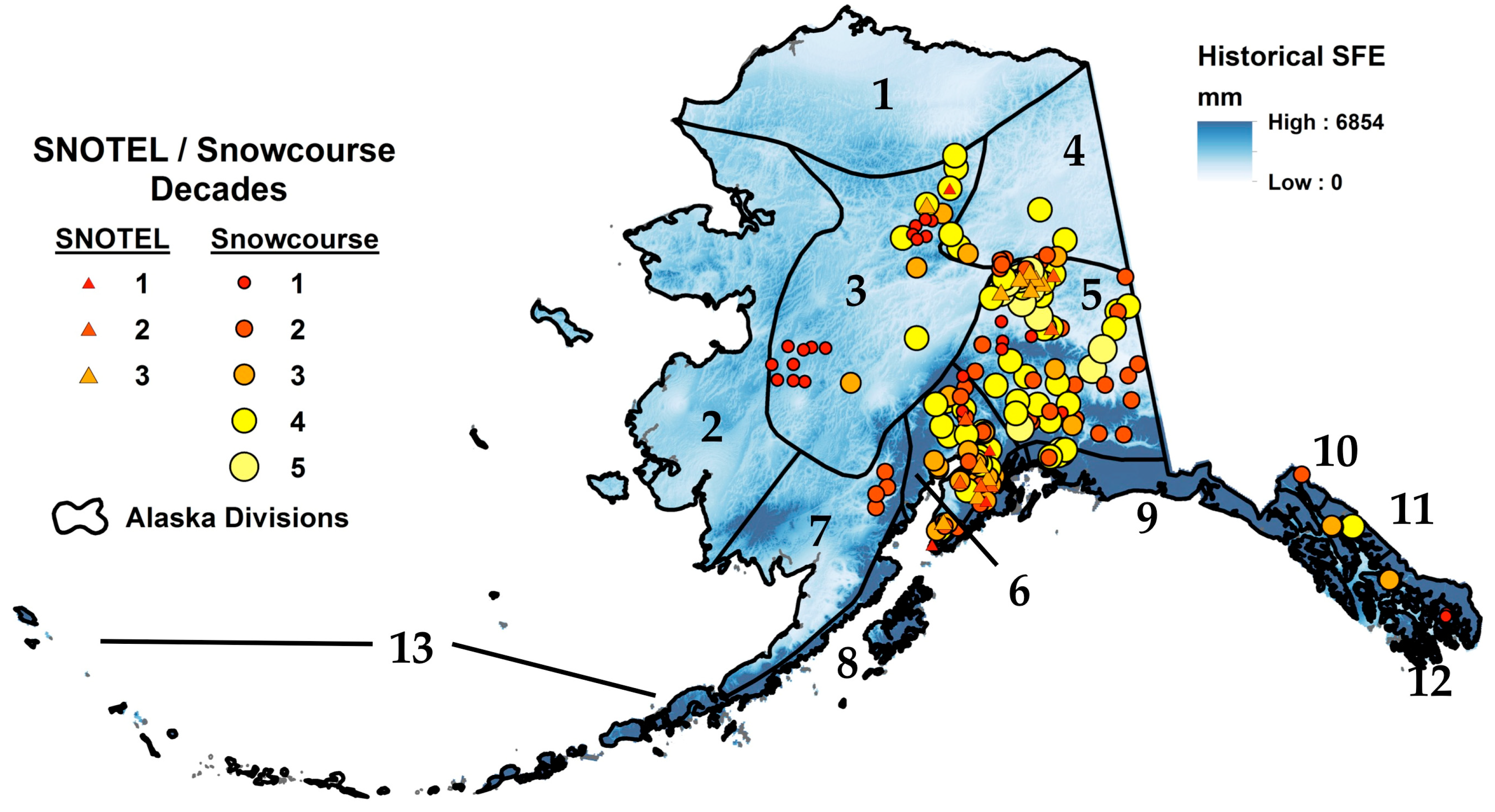
To validate the assumption that SFE from PSF and precipitation is historically equivalent to SWE, we identified 170 snowcourse and 21 Snow Telemetry (SNOTEL) sites that had April 1 SWE for at least seven years in at least one of the decades for which SFE data were available (Figure 1). Decadal average SFE from SNAP data based on CRU TS 3.0 and CRU TS 3.1 were summed from October through March and bilinearly interpolated to the coordinates of each station. These values were compared to April 1 cumulative SWE at all snowcourse and SNOTEL sites. We also compared the two gridded SFE datasets to each other at the snowcourse and SNOTEL [35] site locations. In some cases, snow courses and SNOTEL sites were co-located. In each decade for which data were available (1950–1959 to 1990–1999 for CRU 3.0 [36] and 1950–1959 to 2000–2009 for CRU 3.1 [33]), we calculated the pattern correlation across sites using the Spearman method to account for right-skew in the data, root mean square error (RMSE), mean absolute error (MAE), and bias (average error). We also compared changes in April 1 SWE to changes in cumulative October–March SFE over time at each of the locations that had at least three decades worth of data. Correlations of cumulative October–March SFE over time (Pearson) between the two gridded products were made at each location. We considered the assumption that estimated October–March SFE represents April 1 SWE validated if (1) the Spearman rank correlations between SFE and SWE across the network indicate the two processes were significantly related and (2) the mean absolute errors and calculated biases indicated the error associated with the assumption that SFE ≈ SWE was approximately equal to the error associated with the choice of gridded climatology (e.g., CRU TS 3.0 vs. CRU TS 3.1).

To develop future projections of PSF, SFE, and the ratio of October-to-March SFE to precipitation (SFE:P), we first updated the CMIP3 projections of: (1) PSF developed by McAfee et al. [27] and (2) SFE and SFE:P (after [24], which refers to the ratio as a snow vulnerability index) using CMIP5 projections. We obtained historical and CMIP5 bias corrected delta method downscaled temperature and precipitation projections from SNAP for five GCMs: NCAR CCSM4, NOAA GFDL-CM3, NASA GISS-E2-R, IPSL-CM5ALR, and MRI-CGCM3. Following Walsh et al. [37], Walsh et al. [38] showed these models to perform well over the historical period in the Arctic and Alaska and to represent a range of plausible climate scenarios for the region. We chose to use downscaled projections (771 m decadally averaged monthly values) for RCP 4.5 and RCP 8.5 emissions scenarios. We calculated future PSF as above, and then multiplied it by precipitation to obtain gridded decadal average monthly SFE. We assumed SFE represented an upper estimate of SWE, given no rain-on-snow, melt or redistribution, and used the monthly SFE estimates to calculate SFE:P, the fraction of October-to-March total precipitation potentially stored in spring (April 1) snowpack [30]. After Elsner et al. [39] we defined watersheds with SFE:P ≤ 0.1 as rain dominated, 0.1 < SFE:P < 0.4 as transitional, and SFE:P ≥ 0.4 as snow dominated.

To provide a range of future snow scenarios for Alaska, we calculated changes in PSF, SFE, and SFE:P for 2040–2069 and 2070–2099, relative to a historical period of 1970–1999 CRU TS 3.1 for the 5 GCMs under RCP 4.5 and 8.5 emissions scenarios. We summarized these changes by 12-digit Hydrologic Unit Code watersheds (HUC12, approximately 14,000 in Alaska) and report regional differences in the results by Alaska climate divisions (Figure 1, after Bieniek et al. [40]).

3. Results

Below, we present results validating the assumptions that SFE approximates SWE and describing the responses of PSF, SFE, and SFE:P under future climate changes expected for Alaska relative to temperature and geography.

3.1. Validating Relationships between PSF, SFE, and SWE

Overall, our assumption that modeled SFE approximates observed SWE was validated according to the criteria above. The differences between (1) calculated SFE from CRU TS 3.0 and TS 3.1 (

Table 1. Comparison of cumulative October–March SFE from Climatic Research Unit (CRU) TS 3.0 and CRU TS 3.1-based data at 191 snowcourse/SNOTEL locations. Bias is CRU TS 3.1–CRU TS 3.0.

Decade	Spearman’s ρ	RMSE (mm)	MAE (mm)	Bias (mm)
1950–1959	0.9681	69.99	46.03	36.99
1960–1969	0.9717	66.72	40.69	34.70
1970–1979	0.9834	56.89	29.47	26.87
1980–1989	0.9887	53.30	38.21	37.32
1990–1999	0.9845	50.27	28.77	27.40

), (2) observed SWE from snowcourses and SNOTEL (

Table 2. Comparison of cumulative April 1 snow water equivalent (SWE) at SNOTEL and snowcourse stations to CRU TS 3.0 cumulative October–March SFE. Bias is CRU TS 3.0 SFE–April 1 SWE.

Decade	# Sites	Spearman’s ρ	RMSE (mm)	MAE (mm)	Bias (mm)
1950–1959	1	--	89.01	89.01	−89.01
1960–1969	12	0.9654	50.75	37.96	−37.96
1970–1979	68	0.9363	77.75	47.47	−32.74
1980–1989	115	0.8119	130.25	73.98	−44.64
1990–1999	161	0.8787	107.31	78.74	−57.14

), and (3) modeled SFE and observed SWE (

Table 3. Comparison of cumulative April 1 SWE at SNOTEL and snowcourse stations to CRU 3.1 cumulative October–March SFE. Bias is CRU 3.1 SFE–April 1 SWE.

Decade	# Sites	Spearman’s ρ	RMSE (mm)	MAE (mm)	Bias (mm)
1950–1959	1	--	73.71	73.71	−73.71
1960–1969	12	0.9673	37.42	25.00	2.67
1970–1979	68	0.9270	66.66	37.56	−7.76
1980–1989	115	0.7891	126.65	68.76	−1.821
1990–1999	161	0.8517	109.64	67.42	−28.60
2000–2009	190	0.8364	125.245	80.06	−48.15

) are comparable in magnitude. For example, the difference in estimates of October–March SFE at SNOTEL/snowcourse sites using CRU TS 3.0 and CRU TS 3.1 for 1990–1999 is 27.4 mm, while the difference between SNOTEL/snowcourse April 1 SWE and CRU TS 3.1 for the same period is −28.6 mm. Biases for the different decadal comparisons range from +2.7 to −57.1 mm depending on decade and comparison. However, the range of biases indicate spatial and temporal variation in the outcomes of these comparisons and thus room for further work, particularly on the spatial variability of interactions between synoptic and local determinants of SWE. There is a reasonable representation of spatial patterns in the data, with correlations over 0.75 in all decades, and correlations exceeding 0.9 in the 1960s and 1970s (Table 2). Snowfall equivalent at station locations in the two gridded historical products was highly correlated (Spearman’s ρ > 0.97), although there were substantial differences in the absolute amounts estimated by each. Across all decades, CRU TS 3.1 estimated greater cumulative October–March SFE than CRU TS 3.0 (

Table 4. Comparison of interdecadal variability in April 1 SWE/cumulative October–March SFE.

Comparison	% Locations with Significant Positive Correlations	% Locations with Significant Negative Correlations	% Locations where r ≥ 0.90	% Locations where r ≥ 0.75	% Locations where r ≥ 0.50
CRU 3.0 vs. CRU 3.1	32.98	0	27.239	47.64	68.06
Sites vs. CRU 3.0	0	54.41	10.29	20.59	29.41
Sites vs. CRU 3.1	0.87	51.30	4.35	8.70	23.48

). Cumulative October–March SFE was typically less than April 1 SWE. The biases were smaller in relation to CRU 3.1-derived SFE (Table 3) than to CRU 3.0-derived SFE (Table 2), consistent with the observed differences between the two gridded products.

Correlation coefficients (Table 4) indicate that decadal variation in April 1 SWE at snowcourse and SNOTEL sites was not as well captured by cumulative October–March SFE as were patterns of spatial variability. On the other hand, there were also a number of differences across decades between the two gridded data products, and even some differences between co-located observations (Figure 2). For comparison, there were nine sites with co-located snowcourse and SNOTEL April 1 SWE measurements for at least three overlapping decades. Correlations between April 1 SWE at these co-located snowcourse and SNOTEL sites varied between −0.98 and >0.99. This is likely a function of trying to compare trends in decadal average over only 30 years; when a correlation is performed over only three points, a confidence interval for the coefficient cannot be estimated and even small discrepancies can lead to substantial differences.

3.2. Projected Changes in PSF

PSF decreases universally in Alaska across all future time periods and emissions scenarios investigated. The magnitude and seasonal distribution of the decreases in PSF vary with region, elevation, climate model and RCP emissions scenario because these factors determine the historical baseline and future changes in temperature.

For HUC12 watersheds, the PSF response varies with historical (1980–1999) annual average temperature (Ta, Figure 3). PSF decreases universally, and generally most in the early (autumn) and late (spring) snow season, but the timing of the largest decreases and their relative magnitude also vary. For example, for HUC12 watersheds with historical Ta < −10 °C, decreases in PSF range from 0% to −9% for December to April for all scenarios to nearly −60% for end-of century May under RCP 8.5. As HUC12 historical Ta increases, decreases in PSF occur earlier in the spring and later in the autumn, leading to a contraction of the snow-dominant season. The five-model mean response varies most between November and March for HUC12 near freezing (0 °C < Ta < 2.5 °C). Under RCP 4.5, SFE decreases are about −20% in the 2050s; they increase to around −30% in the 2080s under RCP 8.5. Individual models, however, range from just over −10% to −45% to –50%. Overall, the results indicate a reduction in the length of snow accumulation season and in the amount of highest PSF.

3.3. Projected Changes in SFE

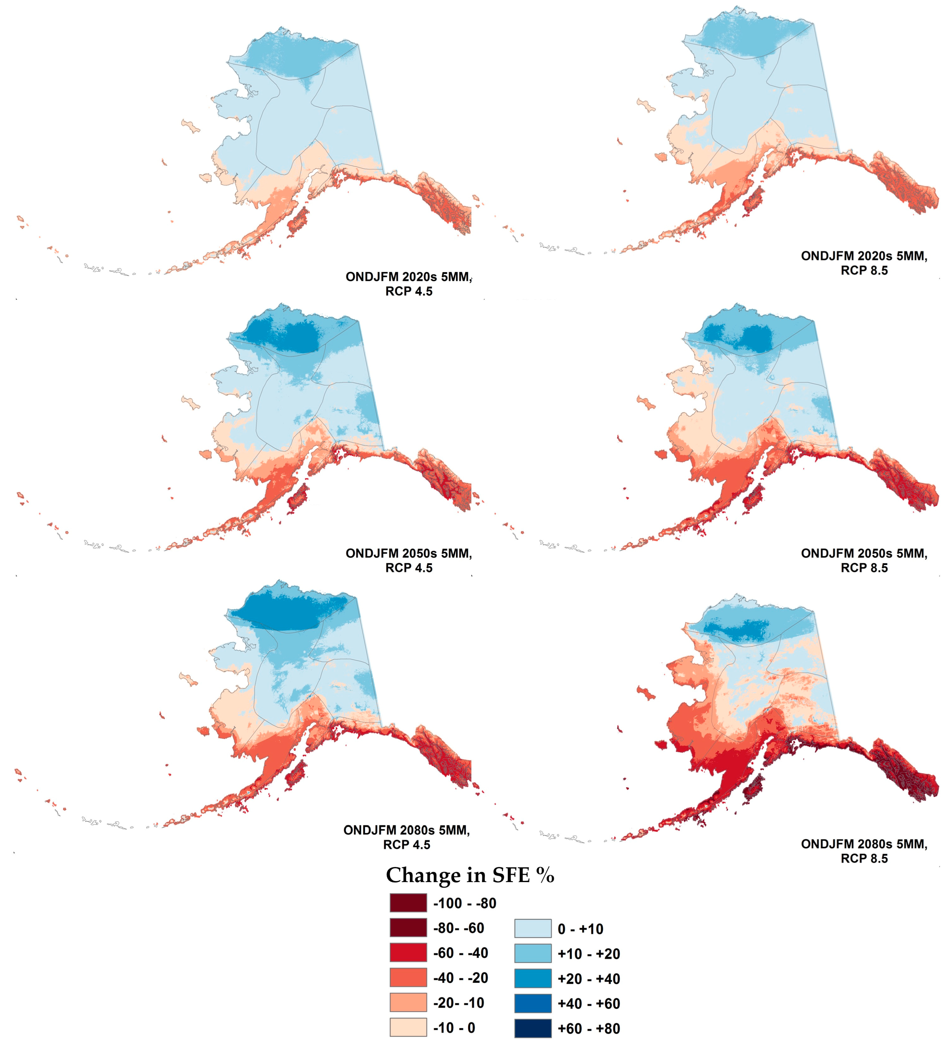
October–March SFE decreases in southeast, southcentral, and southwest Alaska in all composite scenarios (five-model means for RCP 4.5 and 8.5, Figure 4, Table 4) with climate divisions 6–13 averaging −28% for 2040–2069 and −46% for 2070–2099 under the RCP 8.5 emissions scenario. In contrast, SFE increases for the North Slope (Division 1) and Northeast Interior (Division 4) under all scenarios (+19% and +8%, respectively, for 2040–2069 and +15% and +3% for 2070–2099, RCP 8.5) and in Divisions 3 and 5 in all scenarios except 2070–2099 RCP 8.5 (Figure 4,

Table 5. Mean changes in SFE by Alaska Climate Division and climate scenario. All values are mean divisional change in SFE taken across the five Global Climate Model (GCM) composite. See Figure 1 for division locations.

AK Climate Division	Name	2020s		2050s		2080s
		RCP 4.5	RCP 8.5	RCP 4.5	RCP 8.5	RCP 4.5	RCP 8.5
		Mean ΔSFE	Mean ΔSFE	Mean ΔSFE	Mean ΔSFE	Mean ΔSFE	Mean ΔSFE
1	North Slope	11.2	11.1	19.9	18.5	21.9	15.4
2	West Coast	2.2	0.5	2.0	−4.9	−0.5	−18.2
3	Central Interior	5.2	4.4	8.4	5.0	9.0	−1.9
4	Northeast Interior	5.1	4.9	9.8	7.8	10.2	3.0
5	Southeast Interior	3.7	2.9	6.9	4.0	4.4	-6.0
6	Cook Inlet	−4.4	−8.5	−10.8	−19.3	−17.0	−36.8
7	Bristol Bay	−7.6	−12.5	−15.2	−25.4	−22.1	−41.1
8	Northwest Gulf	−16.1	−22.6	−27.8	−38.6	−35.8	−54.9
9	Northeast Gulf	−13.0	−16.7	−20.2	−26.9	−27.7	−46.3
10	North Panhandle	−10.6	−13.2	−15.6	−20.9	−22.7	−42.0
11	Central Panhandle	−13.4	−17.5	−22.8	−29.1	−30.5	−50.8
12	South Panhandle	−17.1	−22.6	−31.1	−37.8	−37.7	−58.0
13	Aleutians	−7.5	−12.3	−15.4	−25.7	−22.8	−41.7

). Mean SFE for Divisions 2, 3, and 5 initially increases modestly as precipitation increases and then decreases with increasing temperatures later in the century.

3.4. Projected Changes in October–March SFE:P Ratio

Most of the area within Alaska climate divisions 1, 3, 4, and 5 continue to receive most of their October–March precipitation as snow until the end of the twenty-first century, although much of the interior becomes progressively less snow dominated in the warmer and end-of-century scenarios (Figure 5). Similar responses dominate in division 2 (West Coast), but the southern part of this division becomes transitional between snow- and rain-dominant by the end of the century.

The rest of the state (southeast, south central, and southwestern Alaska) all become partially and increasingly transitional (SFE:P between 0.1 and 0.4 from the mid-twenty-first century on. By the 2080s under RCP 8.5, the North Slope and the interior divisions remain snow dominated, but the rest of Alaska, on average, is projected to be transitional (

Table 6. Mean SFE:P by Alaska Climate Division and climate scenario. All values are mean divisional change in SFE taken across the five GCM composite. Mean values of SFE:P representing transitional snow hydrology (no longer snow dominated) are in bold italic.

AK Climate Division	Name	2020s		2050s		2080s
		RCP 4.5	RCP 8.5	RCP 4.5	RCP 8.5	RCP 4.5	RCP 8.5
		Mean SFE:P	Mean SFE:P	Mean SFE:P	Mean SFE:P	Mean SFE:P	Mean SFE:P
1	North Slope	98.6	98.5	97.3	96.2	96.3	91.5
2	West Coast	82.1	80.8	77.0	72.0	71.8	59.4
3	Central Interior	90.8	90.1	87.4	84.7	84.0	75.8
4	NE Interior	95.4	95.2	93.2	91.5	91.3	85.4
5	SE Interior	88.7	88.1	85.1	82.8	82.0	74.1
6	Cook Inlet	60.2	57.7	53.0	48.0	47.7	36.6
7	Bristol Bay	57.8	54.9	50.6	44.8	44.5	34.0
8	NW Gulf	43.0	39.9	35.7	30.6	30.7	21.9
9	NE Gulf	51.4	49.6	45.3	42.1	42.1	32.6
10	North Pan.	60.7	59.1	53.8	50.7	50.8	39.1
11	Central Pan.	46.4	44.5	39.4	36.5	36.6	26.9
12	South Pan.	28.8	27.2	23.1	21.1	21.3	14.9
13	Aleutians	58.1	55.3	50.9	45.0	45.1	34.5

). In southeast Alaska, watersheds at sea level become rain dominated by the late twenty-first century. The same is true for parts of southcentral Alaska (Prince William Sound, Kodiak Island, AK, USA) under RCP 8.5 (Figure 5).

Figure 6 illustrates variation in snow responses with elevation, particularly in the mountainous regions of southeast, southcentral, and southwest Alaska where historically snow-dominant or transitional watersheds in mid elevations shift to transitional or rain-dominant watersheds in the 2050s or 2080s, while higher elevation watersheds remain snow dominated.

While SFE:P decreases universally, in southern Alaska climate divisions, the change results in a large fraction of the landscape transitioning from snow dominated SFE:P ratios to transitional SFE:P ratios between the mid-twenty-first century climatology and the 2080s climatology. The changes are most notable in Divisions 6 (Cook Inlet), 8 (Northwest Gulf), and 13 (Aleutians), where from 1970–1999 100%, 81%, and 100%, respectively of the HUC12 watersheds were snow dominated. By the 2080s under RCP 8.5, only 28%, 2%, and 24% of watersheds in those divisions are projected to be snow dominated (

Table 7. Fraction of HUC12 watersheds with snow dominated SFE:P (≥0.4) by Alaska Climate Division and climate scenario.

Division	HUC12 Watersheds	Historical (1970–1999)	2050s		2080s
			RCP 4.5	RCP 8.5	RCP 4.5	RCP 8.5
1	1958	1.00	1.00	1.00	1.00	1.00
2	2382	1.00	1.00	0.99	0.99	0.92
3	2751	1.00	1.00	1.00	1.00	1.00
4	1253	1.00	1.00	1.00	1.00	1.00
5	1759	1.00	1.00	1.00	1.00	1.00
6	672	1.00	0.94	0.80	0.79	0.28
7	1178	1.00	0.75	0.50	0.50	0.33
8	466	0.81	0.27	0.14	0.14	0.02
9	588	0.63	0.42	0.39	0.39	0.28
10	55	1.00	0.89	0.82	0.82	0.53
11	170	0.69	0.44	0.38	0.38	0.18
12	508	0.20	0.08	0.06	0.07	0.01
13	225	1.00	0.88	0.67	0.68	0.24

). Statewide, the mean divisional decrease in SFE:P across snow-dominated watersheds is −35%, but among the southern climate divisions (6–13), it is 56%. Statewide, SFE:P decreases between 3% and 25% in most (59%) HUC12 watersheds, and between 25% and 44% in the remaining (41%) watersheds.

4. Discussion

4.1. Validation of Relationships between PSF, SFE, and SWE

The differences in trend between the historical gridded SFE products and SWE observations could arise from a number of sources. Different gridded precipitation datasets display varied trends, and data from CRU TS products, in particular, contains muted interannual variability [41] that will carry over into gridded SFE. By construction, the gridded SFE data are averages of 10 full years in each decade. We required only seven years of April 1 SWE to estimate a decadal average; missing the April 1 SWE measurement during a single particularly snowy year at the snowcourse or SNOTEL site could lead to a substantial reduction in the observed decadal average. Likewise, the statistical relationship used to characterize decadal average snow-day fraction could be challenged by a decade that included an unusually snowy or dry year. Although this has not been investigated thoroughly in Alaska, over the western U.S. the most extreme snow events contribute enormously to interannual variability [42], and a decadal analysis would likely obscure such detail. There could also be systematic changes in storm or airmass characteristics, such that the validity of the monthly average temperature/snow-day fraction relationship varies over time. This suggests that decadal monthly SFE may not be the best tool for assessing decadal-scale natural variability in April 1 SWE. However, it does appear suitable for investigating spatial patterns in snow characteristics, as well as long-term climate-driven trends, as this does.

There are several reasons SFE would be biased low compared to SWE. In general, point data are not directly comparable to gridded data, as points are rarely representative of the full grid cell [43]. The temperature and precipitation data underlying gridded SFE were derived by interpolation between widely spaced stations [33], so there is likely to be error in the gridded product deriving simply from sparse station coverage. Because each regional PSF relationship with average temperature is the best logistic fit across stations, the statistical relationship between decadal average monthly temperature and PSF also has some error [24], which would contribute to mismatches between the gridded product and site observations. These errors might be expected to be random, but the observations used to develop temperature predictors have a disproportionate contribution from low elevation stations, which could in turn cause larger errors at higher elevations sites with more SWE. In addition, there is a slight temporal offset that cannot be resolved using decadal resolution products. Specifically, cumulative April 1 SWE in the first year of the decade includes a few months from the prior decade (i.e., April 1 SWE in 1980 started accumulating at some time in the late autumn or early winter of 1979). Furthermore, cumulative October–March SFE is not necessarily equivalent to April 1 SWE. At some sites, snowpack may start to accumulate before October 1, so an October–March sum of SFE would underestimate April 1 SWE, although it is worth noting Knowles et al. [30] found no substantial differences in results from including warmer months, and relative contributions of snow to precipitation are less. In addition, SFE does not include the effect of snowpack dynamics, which could lead to increased or decreased SWE relative to SFE. For example, sublimation has been shown to be a significant process in the evolution of snowpack in the Brooks Range [44], and the location of SNOTEL sites in comparatively sheltered locations may hold snow longer than the surrounding landscape and therefore may not be completely representative of grid-scale processes [43]. In the Colorado Rocky Mountains, SNOTEL sites may receive substantially less sublimation than surrounding landscapes, especially forests [45]. These effects could be expected to manifest differently across the range of sites in our study. Finally, we assume in the analyses presented that accumulated snow melts each year, but in glaciated watersheds, this is clearly unrealistic—persistent snow can lead to site SWE available to melt greater than annual SFE.

4.2. Projected Changes in PSF, SFE, and SFE:P

Regional and subregional snow responses to climate change vary with historical mean temperature and elevation, but PSF and SFE:P decrease universally in future scenarios in Alaska. However, there is a clear gradient of future SFE responses across Alaska, from substantial decreases in total seasonal SFE in southeast, southcentral, southwest, and coastal lower elevation Alaska to modest increases in the interior, the North Slope, and at higher elevations. SFE increases occur where projected temperature is still low enough during the cool season for some or all of the projected precipitation increase to arrive as snow. An important distinction here is that the snow season in colder parts of Alaska extends beyond the typical October-March cool season, and comparatively small snow responses but significant shifts in timing can co-occur (e.g., [46]). For example, the North Slope climate division largely has decreases in PSF of 15–25% in May and 30% in October, indicating significant erosion of the snow season, but seasonal SFE increases sufficiently that divisional mean October–March SFE:P remains above 90% even though it decreases more than 7%. Distinguishing between the changes in seasonal timing and the magnitude of seasonal mean changes may be very important for impacts on terrestrial and aquatic systems. Total annual runoff could increase, but changes in the timing of high and low flows could still present challenges for processes adapted to historical timing (e.g., [18]).

The fine-scale projected changes in SFE align well with the 2040–2069 CMIP3 (previous generation climate models) scenario A2 (approximately similar to RCP 8.5) projections of maximum monthly SWE (SWEmax) in Callahan et al. [4], with SWEmax over areas north of the Yukon River increasing by 0–15% and areas south of the Yukon decreasing between 0 and −30%. They generally, but not universally, agree with CMIP5 (14 GCM mean) projections in Maloney et al. [12] for changes in SWE by 2071–2011 relative to 1971–2000 for RCP 8.5. They found decreases in November to May SWE of −10 mm to −40 mm at all Alaska grid cells, especially south of 65 °N. However, they note that at higher latitudes, the transitional area from SWE decreases to increases is subject to the large uncertainty in the magnitude of precipitation increases, which interact with temperature to determine SWE. They also note areas of “spuriously high snow accumulations” that were filtered out of the analysis.

The analyses presented here rely primarily on the five-model mean response for five climate models. Walsh et al. [38] show that the inclusion of a greater number of models would not likely alter mean projected responses, and the five-models serve well to bracket the range of future conditions under the CMIP3 or CMIP5 scenarios and climate models. While the mean scenario may be useful for projecting a range of likely plausible conditions, the dynamics of individual GCMs are not compared here beyond the PSF analysis (Figure 3). A similar analysis for portions of southcentral Alaska based on CMIP3 climate models [24] showed that SFE and SFE:P responses among five climate models generally bracketed the mean response for the 2030–2059 period of analysis. In the analysis presented here, it would be reasonable to substitute the later twenty-first century climatology with higher emissions for a risk-averse (requires more snow) scenario and an earlier climatology with lower emissions for a risk-tolerant (willing to consider less snow) scenario. However, for instances where extremes that derive from seasonal snowpack are of interest, comparing across individual model responses would be preferable for mid-century estimates. By the late twenty-first century, emissions uncertainties are greater than the model uncertainties that dominate mid-century projections [47], so the combined differences between smaller and larger changes in snowpack could be expected to diverge more than implied by the midcentury analysis in [24]. These results also assume the model mean is a bias-free representation of plausible trends, but Brown and Mote [15] showed that climate model simulations underestimated observed decreases in high-latitude snow cover, possibly due to feedbacks in snow-temperature interactions such as snow-albedo feedback. This statistically downscaled product would also be subject to this particular bias.

State-wide local-to-watershed scenarios of future climate impacts on snow and snow hydrology processes are needed for understanding future vulnerability of snow-dependent activities (including subsistence, transportation, infrastructure, and recreation). Improved local-scale projections of changes in snowcover season, snow depth, and water stored in snowpack allow earlier preparation for anticipated impacts or benefits and improved planning for snow-dependent resource management. They are also useful for better understanding hydrologic responses to climate change, particularly if the projections can reliably capture finer spatial and temporal resolution dynamics and better characterization of modeling uncertainties. Our SFE and SFE:P analyses provide an initial step toward characterizing expected changes in Alaskan snow processes, but there are caveats, especially for use in planning or adaptation work. Empirically-derived estimates of SFE from PSF and precipitation are a good first approximation, but they do not account for local factors (such as vegetation, fine scale topography, or wind) that are important for snow redistribution in real landscapes. They also do not account for intra-seasonal factors affecting ultimate snow water equivalent, such as rain-on-snow, sublimation, or melt. While SFE:P is a good indicator of the mean expected seasonal hydrograph, the processes of melt and runoff vary considerably depending on the timing and magnitude of factors affecting melt; moving from snow-dominated to transitional does not imply no years are snow-dominated, or similarly that no years are rain-dominated. Especially in places like southcentral and southwest Alaska where historical snow variation has been high and many watersheds begin to approach or exceed mean annual temperatures near freezing, interannual variability in snowpack development and factors that affect melt may translate to considerable variation in each years’ representativeness of the expected mean scenarios above. For example, interannual and interdecadal variability in Alaska snowdepths are correlated with North Pacific ocean-atmosphere variability indicated by the Pacific North America pattern (PNA, weak to moderate negative November–April correlations in interior and southern Alaska) and Pacific Decadal Oscillation (PDO, moderate to strong negative January–April correlations over all but northern Alaska) [6]. Finally, these projections focus primarily on mean conditions over a climatology, but the annual or even daily extreme events that occur as climate change plays out may be associated with the largest impacts for stakeholders. These extremes have been shown to be more resistant to changes in temperature than mean snowfall [48], implying that a comparable reduction in snow hazards cannot be assumed, and that the influence of climate change on extreme snow responses is likely more difficult to detect.

5. Conclusions

We have shown that SFE developed from gridded PSF and precipitation approximates observed SWE at decadal time scales and the spatial pattern of observed SWE is reasonably captured by historical observations. However, SFE is typically biased low compared to observed SWE, possibly because of our choice of snow season, but also possibly for other reasons including gridded product development. The magnitude bias in any case is similar to the magnitude differences in closely related gridded datasets. Projected changes in October–March PSF, October–March SFE, and SFE:P for Alaska indicate a universal decrease in the length of the snow season and the April 1 SFE:P, but SFE has a more complex response, with large decreases in southern Alaska and at lower elevations and some coastal regions, but modest increases at higher elevations and in the high latitude Arctic because increased precipitation still often falls as snow even in future climates. Historically, most of Alaska was snow dominated, but the area of Alaska considered snow dominated, however, decreases into the future under all scenarios, while transitional and rain-dominated watersheds increase. Gridded products presented here provide a first step toward tools useful for snow-related resource vulnerabilities, but utility for extreme events and interannual variation should be areas targeted for improvement.

References

1. Hinzman, L.D.; Bettez, N.D.; Bolton, W.R.; Chapin, F.S.; Dyurgerov, M.B.; Fastie, C.L.; Griffith, B.; Hollister, R.D.; Hope, A.; Huntington, H.P.; et al. Evidence and Implications of Recent Climate Change in Northern Alaska and Other Arctic Regions. Clim. Chang. 2005, 72, 251–298. [Google Scholar] [CrossRef]
2. Adam, J.C.; Hamlet, A.F.; Lettenmaier, D.P. Implications of global climate change for snowmelt hydrology in the twenty-first century. Hydrol. Process. 2009, 23, 962–972. [Google Scholar] [CrossRef]
3. Euskirchen, E.S.; McGuire, A.D.; Chapin, F.S. Energy feedbacks of northern high-latitude ecosystems to the climate system due to reduced snow cover during 20th century warming. Glob. Chang. Biol. 2007, 13, 2425–2438. [Google Scholar] [CrossRef]
4. Callaghan, T.V.; Johansson, M.; Brown, R.D.; Groisman, P.Y.; Labba, N.; Radionov, V.; Barry, R.G.; Bulygina, O.N.; Essery, R.L.H.; Frolov, D.M.; et al. The Changing Face of Arctic Snow Cover: A Synthesis of Observed and Projected Changes. Ambio 2011, 40, 17–31. [Google Scholar] [CrossRef]
5. Cox, C.J.; Stone, R.S.; Douglas, D.C.; Stanitski, D.M.; Divoky, G.J.; Dutton, G.S.; Sweeney, C.; George, J.C.; Longenecker, D.U. Drivers and Environmental Responses to the Changing Annual Snow Cycle of Northern Alaska. Bull. Am. Meteorol. Soc. 2017, 98, 2559–2577. [Google Scholar] [CrossRef]
6. Ge, Y.; Gong, G. North American Snow Depth and Climate Teleconnection Patterns. J. Clim. 2009, 22, 217–233. [Google Scholar] [CrossRef]
7. Mudryk, L.R.; Kushner, P.J.; Derksen, C. Interpreting observed northern hemisphere snow trends with large ensembles of climate simulations. Clim. Dyn. 2014, 43, 345–359. [Google Scholar] [CrossRef]
8. Rupp, D.E.; Mote, P.W.; Bindoff, N.L.; Stott, P.A.; Robinson, D.A. Detection and Attribution of Observed Changes in Northern Hemisphere Spring Snow Cover. J. Clim. 2013, 26, 6904–6914. [Google Scholar] [CrossRef]
9. Stone, R.S.; Dutton, E.G.; Harris, J.M.; Longenecker, D. Earlier spring snowmelt in northern Alaska as an indicator of climate change. J. Geophys. Res. Atmos. 2002, 107, ACL 10-1–ACL 10-13. [Google Scholar] [CrossRef]
10. Brown, R.D.; Robinson, D.A. Northern Hemisphere spring snow cover variability and change over 1922–2010 including an assessment of uncertainty. Cryosphere 2011, 5, 219–229. [Google Scholar] [CrossRef] [Green Version]
11. Liston, G.E.; Hiemstra, C.A.; Liston, G.E.; Hiemstra, C.A. The Changing Cryosphere: Pan-Arctic Snow Trends (1979–2009). J. Clim. 2011, 24, 5691–5712. [Google Scholar] [CrossRef]
12. Maloney, E.D.; Camargo, S.J.; Chang, E.; Colle, B.; Fu, R.; Geil, K.L.; Hu, Q.; Jiang, X.; Johnson, N.; Karnauskas, K.B.; et al. North American Climate in CMIP5 Experiments: Part III: Assessment of Twenty-First-Century Projections. J. Clim. 2014, 27, 2230–2270. [Google Scholar] [CrossRef]
13. Bintanja, R.; Andry, O. Towards a rain-dominated Arctic. Nat. Clim. Chang. 2017, 7, 263–267. [Google Scholar] [CrossRef]
14. Räisänen, J. Warmer climate: Less or more snow? Clim. Dyn. 2008, 30, 307–319. [Google Scholar] [CrossRef]
15. Brown, R.D.; Mote, P.W. The Response of Northern Hemisphere Snow Cover to a Changing Climate. J. Clim. 2009, 22, 2124–2145. [Google Scholar] [CrossRef]
16. Barnett, T.P.; Adam, J.C.; Lettenmaier, D.P. Potential impacts of a warming climate on water availability in snow-dominated regions. Nature 2005, 438, 303–309. [Google Scholar] [CrossRef] [PubMed]
17. Berghuijs, W.R.; Woods, R.A.; Hrachowitz, M. A precipitation shift from snow towards rain leads to a decrease in streamflow. Nat. Clim. Chang. 2014, 4, 583–586. [Google Scholar] [CrossRef]
18. Beamer, J.P.; Hill, D.F.; McGrath, D.; Arendt, A.; Kienholz, C. Hydrologic impacts of changes in climate and glacier extent in the Gulf of Alaska watershed. Water Resour. Res. 2017, 53, 7502–7520. [Google Scholar] [CrossRef]
19. McKelvey, K.S.; Copeland, J.P.; Schwartz, M.K.; Littell, J.S.; Aubry, K.B.; Squires, J.R.; Parks, S.A.; Elsner, M.M.; Mauger, G.S. Climate change predicted to shift wolverine distributions, connectivity, and dispersal corridors. Ecol. Appl. 2011, 21, 2882–2897. [Google Scholar] [CrossRef]
20. Young-Robertson, J.M.; Bolton, W.R.; Bhatt, U.S.; Cristóbal, J.; Thoman, R. Deciduous trees are a large and overlooked sink for snowmelt water in the boreal forest. Sci. Rep. 2016, 6, 29504. [Google Scholar] [CrossRef] [PubMed]
21. Hassol, S.; Arctic Climate Impact Assessment; Arctic Monitoring and Assessment Programme; Program for the Conservation of Arctic Flora and Fauna; International Arctic Science Committee. Impacts of a Warming Arctic: Arctic Climate Impact Assessment; Cambridge University Press: Cambridge, UK, 2004; ISBN 0521617782. [Google Scholar]
22. Euskirchen, E.S.; Goodstein, E.S.; Huntington, H.P. An estimated cost of lost climate regulation services caused by thawing of the Arctic cryosphere. Ecol. Appl. 2013, 23, 1869–1880. [Google Scholar] [CrossRef] [PubMed]
23. Hayward, G.H.; Colt, S.; McTeague, M.L.; Hollingsworth, T.N. Climate change vulnerability assessment for the Chugach National Forest and the Kenai Peninsula. In General Technical Report PNW-GTR-950; U.S. Department of Agriculture, Forest Service Pacific Northwest Reserach Station: Portland, OR, USA, 2017; Volume 950, 340p. [Google Scholar]
24. Littell, J.S.; McAfee, S.A.; O’Neel, S.; Sass, L.; Burgess, E.; Colt, S.; Clark, P. Chapter 3: Snow and Ice. In Climate Change Vulnerability Assessment for the Chugach National Forest and the Kenai Peninsula; Hayward, G.D., Colt, S., McTeague, M.L., Hollingsworth, T.N., Eds.; U.S. Department of Agriculture: Portland, OR, USA, 2017; pp. 29–77. [Google Scholar]
25. National Oceanic and Atmospheric Administration (NOAA); National Centers for Environmental Information (NCEI). Data Tools: Local Climatological Data. Available online: https://www.ncdc.noaa.gov/cdo-web/datatools/lcd (accessed on 23 March 2018).
26. Salzmann, N.; Huggel, C.; Rohrer, M. Data and knowledge gaps in glacier, snow and related runoff research—A climate change adaptation perspective. J. Hydrol. 2014, 518, 225–234. [Google Scholar] [CrossRef]
27. McAfee, S.A.; Walsh, J.; Rupp, T.S. Statistically downscaled projections of snow/rain partitioning for Alaska. Hydrol. Process. 2014, 28, 3930–3946. [Google Scholar] [CrossRef]
28. Kienzle, S.W. A new temperature based method to separate rain and snow. Hydrol. Process. 2008, 22, 5067–5085. [Google Scholar] [CrossRef]
29. Legates, D.R.; Bogart, T.A.; Legates, D.R.; Bogart, T.A. Estimating the Proportion of Monthly Precipitation that Falls in Solid Form. J. Hydrometeorol. 2009, 10, 1299–1306. [Google Scholar] [CrossRef]
30. Knowles, N.; Dettinger, M.D.; Cayan, D.R. Trends in Snowfall versus Rainfall in the Western United States. J. Clim. 2006, 19, 4545–4559. [Google Scholar] [CrossRef]
31. Scenarios Network For Alaska and Arctic Planning, University of Alaska. Historical Monthly and Derived Precipitation Products—771 m CRU TS. 2014. Available online: http://ckan.snap.uaf.edu/dataset/historical-monthly-and-derived-precipitation-products-771m-cru-ts (accessed on 4 November 2016).
32. Scenarios Network for Alaska and Arctic Planning, University of Alaska. Historical Monthly and Derived Temperature Products—771 m CRU TS. 2014. Available online: http://ckan.snap.uaf.edu/dataset/historical-monthly-and-derived-temperature-products-771m-cru-ts (accessed on 4 November 2016).
33. Harris, I.; Jones, P.D.; Osborn, T.J.; Lister, D.H. Updated high-resolution grids of monthly climatic observations—The CRU TS 3.10 Dataset. Int. J. Climatol. 2014, 34, 623–642. [Google Scholar] [CrossRef] [Green Version]
34. Daly, C.; Gibson, W.P.; Taylor, G.H.; Johnson, G.L.; Pasteris, P. A knowledge-based approach to the statistical mapping of climate. Clim. Res. 2002, 22, 99–113. [Google Scholar] [CrossRef]
35. Schaefer, G.L.; Paetzold, R.F. SNOTEL (SNOwpack TELelemetry) and SCAN (Soil Climate Analysis Network). In Proceedings of the International Workshop on Automated Weather Stations for Applications in Agriculture and Water Resources Management, 2001. Available online: http://citeseerx.ist.psu.edu/viewdoc/download?doi=10.1.1.177.966&rep=rep1&type=pdf (accessed on 3 May 2018).
36. Mitchell, T.D.; Jones, P.D. An improved method of constructing a database of monthly climate observations and associated high-resolution grids. Int. J. Climatol. 2005, 25, 693–721. [Google Scholar] [CrossRef]
37. Walsh, J.E.; Chapman, W.L.; Romanovsky, V.; Christensen, J.H.; Stendel, M. Global Climate Model Performance over Alaska and Greenland. J. Clim. 2008, 21, 6156–6174. [Google Scholar] [CrossRef]
38. Walsh, J.E.; Bhatt, U.S.; Littell, J.S.; Leonawicz, M.; Lindgren, M.; Kurkowski, T.A.; Bieniek, P.; Thoman, R.; Gray, S.T.; Rupp, T.S. Downscaling of climate model output for Alaskan stakeholders. Environ. Model. Softw. 2018, in press. [Google Scholar] [CrossRef]
39. Elsner, M.M.; Cuo, L.; Voisin, N.; Deems, J.S.; Hamlet, A.F.; Vano, J.A.; Mickelson, K.E.B.; Lee, S.Y.; Lettenmaier, D.P. Implications of twenty-first century climate change for the hydrology of Washington State. Clim. Chang. 2010, 102, 225–260. [Google Scholar] [CrossRef]
40. Bieniek, P.A.; Bhatt, U.S.; Thoman, R.L.; Angeloff, H.; Partain, J.; Papineau, J.; Fritsch, F.; Holloway, E.; Walsh, J.E.; Daly, C.; et al. Climate Divisions for Alaska Based on Objective Methods. J. Appl. Meteorol. Climatol. 2012, 51, 1276–1289. [Google Scholar] [CrossRef]
41. McAfee, S.A.; Guentchev, G.; Eischeid, J. Reconciling precipitation trends in Alaska: 2. Gridded data analyses. J. Geophys. Res. Atmos. 2014, 119. [Google Scholar] [CrossRef]
42. Lute, A.C.; Abatzoglou, J.T. Role of extreme snowfall events in interannual variability of snowfall accumulation in the western United States. Water Resour. Res. 2014, 50, 2874–2888. [Google Scholar] [CrossRef]
43. Meromy, L.; Molotch, N.P.; Link, T.E.; Fassnacht, S.R.; Rice, R. Subgrid variability of snow water equivalent at operational snow stations in the western USA. Hydrol. Process. 2013, 27, 2383–2400. [Google Scholar] [CrossRef]
44. Liston, G.E.; Sturm, M. The role of winter sublimation in the Arctic moisture budget. Nord. Hydrol. 2004, 35, 325–334. [Google Scholar] [CrossRef]
45. Sexstone, G.A.; Clow, D.W.; Fassnacht, S.R.; Liston, G.E.; Hiemstra, C.A.; Knowles, J.F.; Penn, C.A. Snow Sublimation in Mountain Environments and Its Sensitivity to Forest Disturbance and Climate Warming. Water Resour. Res. 2018, 54, 1191–1211. [Google Scholar] [CrossRef]
46. McGrath, D.; Sass, L.; O’Neel, S.; Arendt, A.; Kienholz, C. Hypsometric control on glacier mass balance sensitivity in Alaska and northwest Canada. Earth’s Future 2017, 5, 324–336. [Google Scholar] [CrossRef]
47. Hawkins, E.; Sutton, R. The Potential to Narrow Uncertainty in Regional Climate Predictions. Bull. Am. Meteorol. Soc. 2009, 90, 1095–1108. [Google Scholar] [CrossRef]
48. O’Gorman, P.A. Contrasting responses of mean and extreme snowfall to climate change. Nature 2014, 512, 416–418. [Google Scholar] [CrossRef] [PubMed]
Figure 1. Snow Telemetry (SNOTEL, 21 total) and snowcourse sites (170 total) used in this study, 13 Alaska climate divisions (black boundaries), and 1970–1999 historical snowfall equivalent (SFE). See Table 5 for division names.
Water 10 00668 g001
Figure 2. Correlation (Pearson) between the April 1 SWE measured over at least three decades at co-located SNOTEL and snowcourse sites. Teuchet Creek through Fairbanks F.O. are in the northwest part of Alaska Division 5; Cooper Lake though Indian Pass are in southern Alaska Division 6; Bettles Field is in Division 3.
Water 10 00668 g002
Figure 3. 2050s and 2080s means and ranges of projected monthly projected snow day fraction (PSF) change scenarios. Each panel represents mean projected changes extracted from Alaska 12-digit Hydrologic Unit Code (HUC12) watersheds in the 1970–1999 mean annual temperature (Ta) within the indicated range. Ranges include projections from Representative Concentration Pathway (RCP) 4.5 and RCP 8.5. Percent values indicate the percentage of Alaska’s area in each of the temperature categories.
Water 10 00668 g003
Figure 4. 2020s (top), 2050s (middle), and 2080s (bottom) changes in five-model mean projected October–March SFE for RCP 4.5 (left) and RCP 8.5 (right). Climate division boundaries appear as gray lines.
Water 10 00668 g004
Figure 5. 2020s, 2050s, and 2080s five-model mean projected October–March SFE:P ratio for RCP 4.5 (left) and RCP 8.5 (right).
Water 10 00668 g005
Figure 6. HUC12 watershed mean elevation versus five-model mean projected October–March SFE:P ratio for RCP 8.5. SFE:P is expressed in percent. Alaska Climate Division 6 (Cook Inlet, left), Divisions 7 and 8 (center), and Divisions 9–12 (right) for historical (top row), 2050s (middle row) and 2080s (bottom row).
Water 10 00668 g006