Article

Multi-Source Uncertainty Analysis in Simulating Floodplain Inundation under Climate Change

1
Institute for Landscape Ecology and Resources Management (ILR), Research Centre for BioSystems, Land Use and Nutrition (iFZ), Justus Liebig University Giessen, Heinrich-Buff-Ring 26, 35392 Giessen, Germany
2
Centre for International Development and Environmental Research (ZEU), Justus Liebig University Giessen, Senckenbergstraße 3, 35390 Giessen, Germany
*
Author to whom correspondence should be addressed.
Water 2018, 10(6), 809; https://doi.org/10.3390/w10060809
Submission received: 30 May 2018 / Revised: 14 June 2018 / Accepted: 15 June 2018 / Published: 19 June 2018
(This article belongs to the Section Hydrology)

Abstract

:
Floodplains are highly complex and dynamic systems in terms of their hydrology. Thus, they harbor highly specialized floodplain plant species depending on different inundation characteristics. Climate change will most likely alter those characteristics. This study investigates the potential impact of climate change on the inundation characteristics of a floodplain of the Rhine River in Hesse, Germany. We report on the cascading uncertainty introduced through climate projections, climate model structure, and parameter uncertainty. The established modeling framework integrates projections of two general circulation models (GCMs), three emission scenarios, a rainfall–runoff model, and a coupled surface water–groundwater model. Our results indicate large spatial and quantitative uncertainties in the simulated inundation characteristics, which are mainly attributed to the GCMs. Overall, a shift in the inundation pattern, possible in both directions, and an increase in inundation extent are simulated. This can cause significant changes in the habitats of species adapted to these highly-endangered ecosystems.

1. Introduction

The ecohydrology of floodplains is highly influenced by regular floods, defined by characteristics such as the height of the water level, flood duration, and recurrence intervals [1,2,3,4,5]. Consequently, a wide habitat heterogeneity exists and species which are highly-specialized on the present conditions can be found in these ecosystems [6,7]. Apart from providing habitats for plants and breeding birds or fish, floodplains provide many other ecosystem services, including the regulation of floods, water supply, and nutrient retention [8]. At the same time, floodplains are among the most-endangered ecosystems worldwide [9]. Flow regulation and damming, urban sprawl, and agricultural land use change have resulted in disconnected floodplains that can no longer sustain their original services.
Climate change is likely to have additional effects on floodplains and their functionality due to general changes in the hydrological cycle [10]. More precisely, the seasonality and extremes of low and high flows will be altered [11,12,13]. As flood characteristics are changed, a shift in habitat availability and species distribution is expected [14,15,16,17].
Reconnecting floodplains to rivers is promoted as a key to restore floodplains’ functionalities [9,18]. A common way to develop restoration plans or assess the effect of management options is through model projections. Floodplains should be simulated with fully-integrated models that consider surface water–groundwater interactions to capture all relevant ecohydrological processes [19,20,21]. These models can enhance the understanding of the hydrological functions of floodplains and can provide insight into the potential impacts of climate change [17,22,23].
Studies of climate change impact involve several cascading uncertainties related to the climate model itself, the emission scenario, hydrological model structure and parameters, spatial model input data, and initial conditions [24,25,26,27,28,29]. Studies have rarely considered the propagation of the uncertainty from climate projections to rainfall–runoff models and flood inundation models [30,31]. One of the few existing modeling studies on climate change impacts on floodplains was carried out by Sorribas et al. [32], who focused on the changes of discharge, inundation extent, and the uncertainty introduced by the general circulation model (GCM) in the Amazon. Thompson et al. [17] used a coupled hydrological/hydraulic model (MIKE SHE/MIKE 11) to assess the impact of climate change on wet grassland in lowlands for different emission scenarios. Finally, Barron et al. [33] investigated the impact on groundwater-dependent terrestrial vegetation using rainfall–runoff and groundwater models with data from 15 GCMs but did not consider any further sources of uncertainty.
This paper addresses this gap by studying the cascading effect of projected climate change impact on inundation frequency and duration on a floodplain of the Rhine River in Germany. We investigate the uncertainty through the modeling chain of a rainfall–runoff model Hydrologiska Byråns Vattenbalansavdelning (HBV) and a coupled parsimonious surface water–groundwater model (catchment modeling framework (CMF)). For this, we use projections of two GCMs and three emission scenarios as driving forces for HBV to simulate the future discharge of the Rhine. The generated discharge time series by the rainfall–runoff model are then used to drive the surface water–groundwater model in order to project spatially-distributed flood characteristics in a specific floodplain of the Rhine and identify the uncertainties in the modeling procedure.
The guiding questions for our research are as follows: How are the changes in inundation characteristics related to the river discharge projections? How will the spatial distributions of inundation characteristics change on a small scale and through time? What are the main sources causing differences related to the projected inundation characteristics, and how is the uncertainty propagating throughout the modeling framework?

2. Materials and Methods

2.1. Study Site

The floodplain ‘‘Knoblochsaue’’ is located on the right bank of the Rhine, approximately 30 km southwest of Frankfurt in the Federal State of Hesse, Germany (49°49′ N, 88°6′ E). The floodplain is part of the nature reserve Kühkopf-Knoblochsaue, the largest of its type in Hesse (Figure 1). The nature reserve is of particular importance for rare and endangered flora and fauna and is protected by the European Habitats Directive (Council Directive 92/43/EEC). The study area is approximately 14.9 km2. As the floodplain is frequently flooded, embankment protects a subarea of about 6.4 km2 from inundations. This area is also referred to as the inactive floodplain.
Annual precipitation is about 618 mm and the mean daily temperature is about 10.7 °C (observed at the station Darmstadt (49°52′ N, 8°40′ E) by the German meteorological service) between the years 1981 and 2010. Daily water levels measurements for the Rhine are available for the gauging station Nierstein Oppenheim (49°51′ N, 8°21′ E; approximately 3.5 km downstream the study area). Average discharge between 2000 and 2014 was 1673 m3 s−1 (90% quantile: 2460 m3 s−1; 10% quantile: 1010 m3 s−1).

2.2. Surface Water–Groundwater Model

For this study, we modified a previously-developed parsimonious, physically-based surface water–groundwater model to simulate flood characteristics in the floodplain [34]. The model is built with the catchment modeling framework (CMF), version v0.1315 [35,36] and includes the interaction between surface water and groundwater flow. CMF is a flexible modular framework suitable for different hydrological model structures (from detailed mechanistic to lumped large-scale linear storage-based models). The models differ in their number and connectivity of water storages as well as in the type of equation calculating the water fluxes between the components. In order to implement an irregular grid for the lateral spatial discretization, CMF is based on the concept of finite volumes for discretizing continuous water storages [37].
The study area is divided into 272 irregular polygons with different sizes (336–480,000 m2) based on similar elevation and land use (Figure 1 right). Land use was divided into six classes (stream, water body, agriculture, meadow, forest and urban area). The standard deviation of the elevation in one polygon was kept at a maximum of 2.3 m (mean: 0.5 m).
A vertical discretization is not considered to simplify the model. The model is forced by the daily water level of the stream and the groundwater level at the upslope edge of the study area, both set as a dynamic Dirichlet boundary condition. Precipitation and modeled evapotranspiration using the FAO guidelines [38] complement the system boundaries. More details about the study area and the model set up, including the surface water routines, can be found in Maier et al. [34].
To reduce the amount of forcing data, we replaced the upslope boundary condition with a no-flow boundary. A subsequent recalibration of the model resulted in similar optimal parameter sets and an increase of the RMSE of less than 0.1 m in the active floodplain. We tested several CMF parameter sets from Maier et al. [34] for numerical stability. Due to the numerical stability and computation effort, we selected only one parameter set. The parameter set defines the soil properties as follows: 2830 m/d for hydraulic conductivity, 0.3 m3/m3 for porosity, 0.23 m3/m3 for residual wetness, and 7.4 m for soil thickness.

2.3. Water Level Forcing

For CMF forcing, we need stream water level data. Measured data are used for current conditions, and we use projected data for our future climate scenarios. We applied the rainfall–runoff model (HBV) [39,40] in a modified version [41] as a conceptual semi-distributed hydrological model to simulate the discharge of the Rhine River. It has been shown in recent comparison studies that HBV gives satisfactory results using various model performance criteria for the Rhine River [42,43]. Based on these studies and a previous study from Vetter et al. [44], in which a minor part of the overall uncertainty was shown to be related to hydrological models, we only consider the HBV model to simulate discharge in the Rhine River and no further hydrological multi-model ensemble. We then transformed discharge projections from HBV to water levels by existing, calibrated, and validated rating curves.
The HBV model was set up for the Rhine catchment at the Mainz gauging station, which was separated into six sub-catchments. This subdivision was done in order to include different climatic conditions. For the semi-lumped model, only one parameter set for the entire catchment was considered.
We considered both the parameter and predictive model uncertainty of HBV. To capture the parameter uncertainty, the GLUE methodology [45] was applied. Accordingly, we ran the model 100,000 times following a Latin hypercube procedure using SPOTPY [46] with all the 12 input model parameters of HBV (Table A1). We used the Nash–Sutcliffe (NSE) coefficient [47] as the objective function in order to focus the model performance investigation on the high flows, which are of course the most important source for flooding. As behavioral runs, we chose the top 10% of all model runs, resulting in an acceptable threshold of NSE > 0.72. We projected the discharge with the parameter sets defined as acceptable for each climate scenarios. The years 2001 to 2009 were used as the calibration period and 2010 to 2013 as the validation period. Further, we used the 5th and 95th percentiles over each simulation and over each time step as the synthetic minimum and maximum water levels for the corresponding climate projection. The approach for the predictive uncertainty is based on heteroscedastic error modeling that represents the aggregated effects of data and model structural errors of the best model run found [48]. We applied the Box–Cox [49] transformations with a fixed transformation value of λ = 0.5 to get a robust statistical model for the residuals of discharge simulations. We ran the analysis with the best performing model run in a post-processing mode and checked our results for normality. However, we did not treat any potential autocorrelation effects in the residuals, which might result in an over-estimation of the predictive uncertainty [48]. The defined parameters for the transformation equation are then applied to the simulations under the climate change scenarios. Again, we used the 5th and the 95th percentiles of the predictive uncertainty as discharge projections. Additionally, we performed simulations with the best-performing HBV model.

2.4. Climate Forcing

We selected two general circulation models (GCMs) from the Coupled Model Intercomparison Project Phase 5 (CMIP5) [50]: HadGEM2-ES from the Met Office Hadley Centre and MPI-ESM-LR from the Max Planck Institute for Meteorology. In recent studies, McSweeney et al. [51] concluded that both GCMs perform satisfactorily for Europe, and Brands et al. [52] showed that both models outperform the remaining models by reproducing the present climate conditions in Europe and Africa. Other than that, the two GCMs show differences in the annual mean temperature and annual mean precipitation in the contributing catchment area of the Rhine. The model HadGEM shows a larger annual mean temperature change and a larger decrease in the annual mean precipitation especially in summer and autumn when compared to MPI-ESM-LR [53,54]. Both models consider three representative concentration pathways (RCP), i.e., the RCP 2.6 (low concentration), RCP 4.5 (medium concentration), and RCP 8.5 (high concentration).
Subsequently, we obtained six different climate projections from the combination of the GCMs and RCPs. The quantile mapping method [55,56] was used to downscale the daily precipitation and temperature time series projections. We used quantile mapping for bias correction for two reasons. First, the uncertainty related to the GCMs is larger than the uncertainty associated with the downscaling and bias-correction method [25,57,58]. Second, the quantile mapping method is reviewed by several authors in the context of hydrological impacts studies as a preferable method [56,59,60,61]
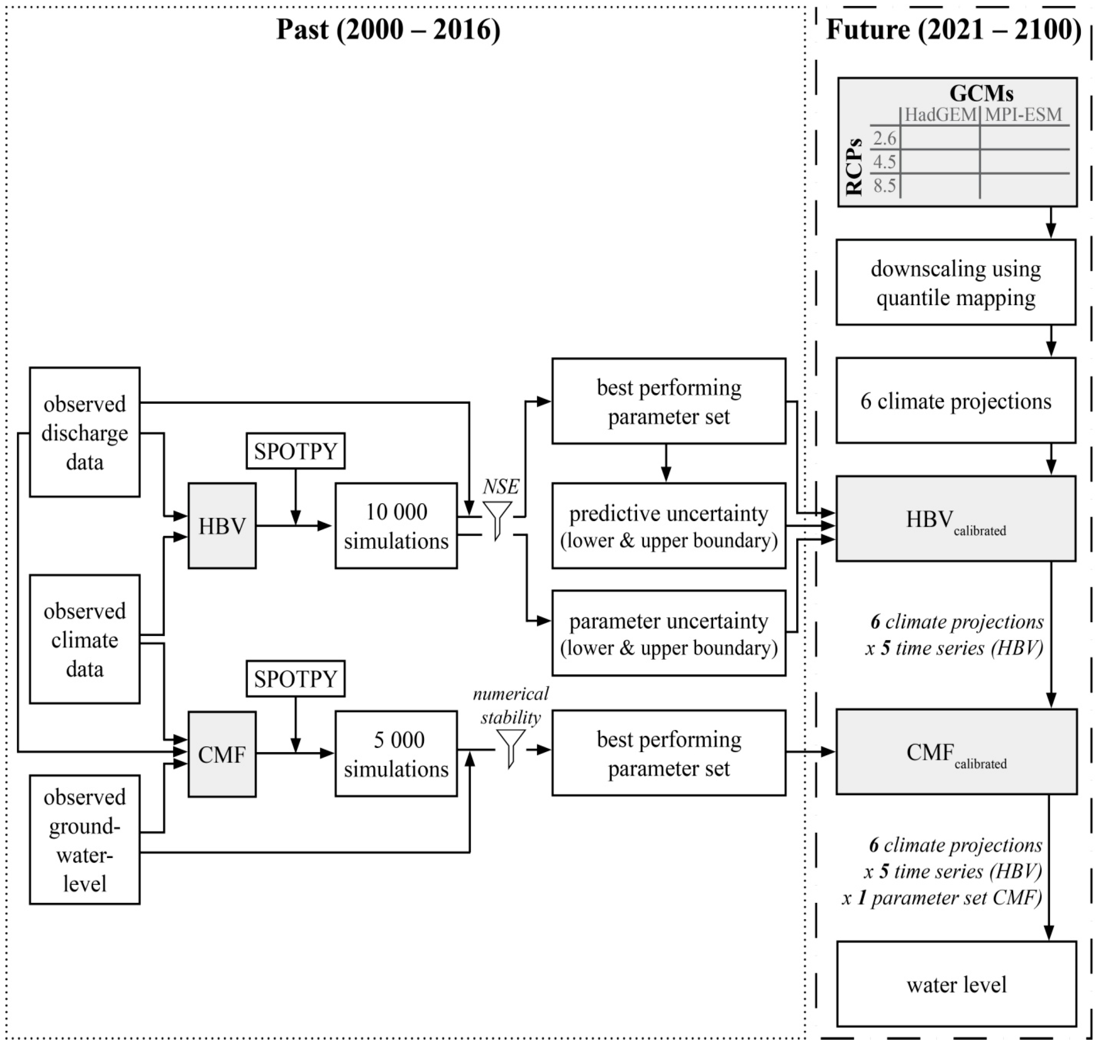
This overall set-up results in 30 simulations of the CMF model for future projections through the combination of five projected water level time series derived from the HBV model (best-performing simulation, 5th and 95th percentiles of parameter and predictive uncertainty), the two GCMs (HadGEM and MPI-ESM), and the three RCPs (RCP 2.6, RCP 4.5, RCP 8.5). A summarizing figure of the methodology and the consecutive steps used is given in Figure 2.
The reference height of a polygon is given by its average height over the entire polygon; i.e., each polygon is represented by one defined surface height. We define inundation as a water level of 0.05 m above the surface. For the following description of inundation in the study area, we used two inundation characteristics: the number of inundation days per year and the mean duration of an inundation period. Those metrics are useful when considering further consequences for example for flood meadow species composition, as those are influences by the inter-annual variation of flooding and droughts and the duration of flooding [62,63].

3. Results

3.1. Projection of the Rhine River Water Level

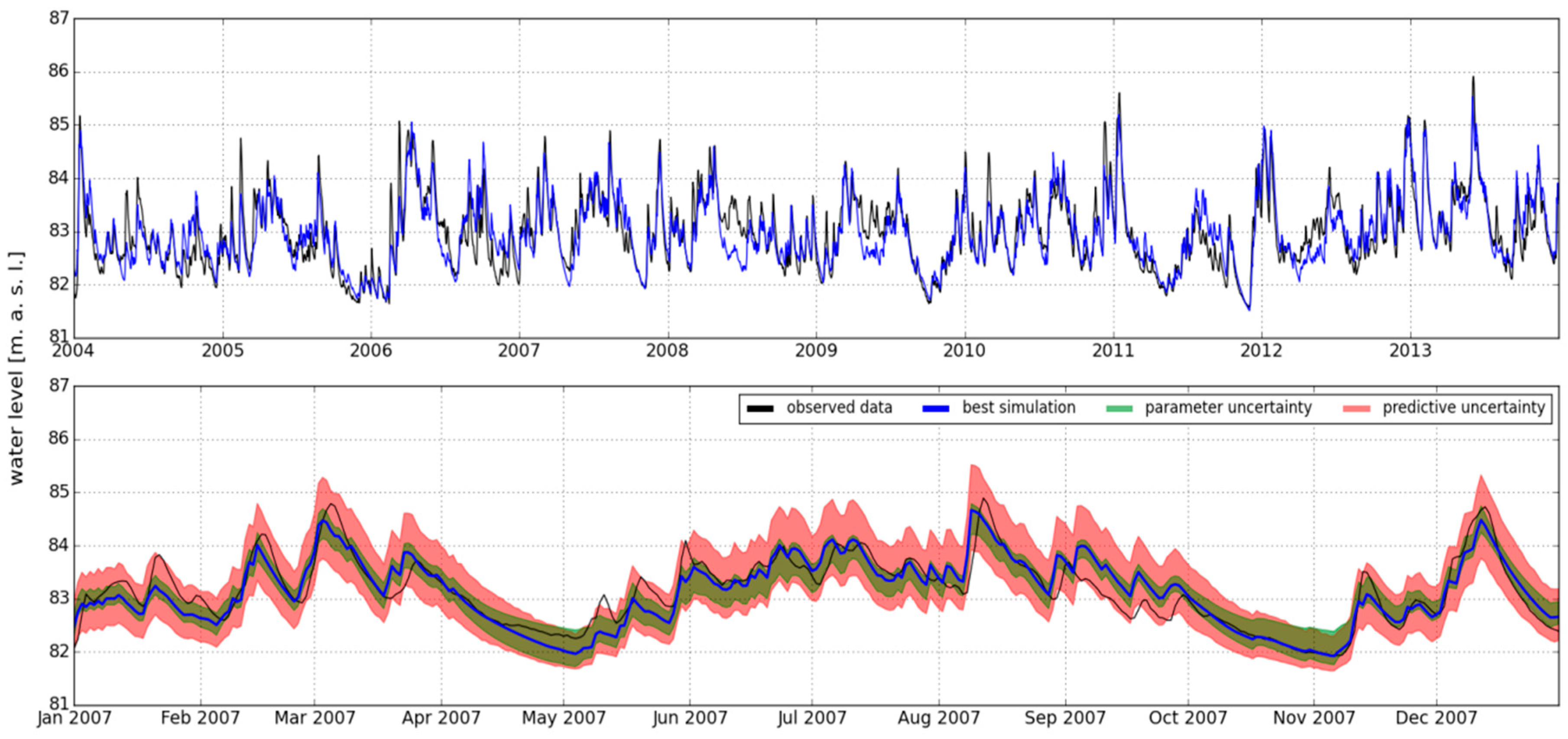
The NSE for daily discharge during the calibration (2001–2009) and validation period (2010–2013) of the HBV model is 0.79 and 0.82, respectively (Appendix A, Figure A2). Slightly worse results of the HBV-model can be found if only the high flows are considered (NSE: 0.54 for 70th percentile based on observed discharge). In the next step, we forced the calibrated model with bias corrected precipitation and temperature data from the two GCMs (HadGEM2-ES and MPI-ESM-LR) and the three RCPs (RCP 2.6, RCP 4.5 and RCP 8.5) to project future runoff. From these, we derived projected water levels (Figure 3).
Figure 3 shows the simulated past and future water levels of the Rhine per month. Additionally, the trends and absolute changes in mean water level are given below each box plot. Until 2050, all months except January, May, June, and December show an increase between 0.55 m and 2.06 m in the mean water level for almost all GCMs–RCPs combinations. In January, there is a small decrease in the water level (up to 0.45 m). The end-century period primarily shows the same pattern. However, some future projections turn from an increasing or no trend to no trend or a decreasing trend until the end of the end-century period. It should be noted that the total range of water levels decreases in almost all future projections compared to the past. An over 50% decrease in the water level range for single months compared to the past can be seen in January, May, June, October, November, and December. Comparing the two climate scenarios, it is striking that the mean water levels of the MPI-ESM model are always below those of the HadGEM model. At the same time, there is no clear pattern in either increasing or decreasing water level changes from the low concentration pathway (RCP 2.6) to the high concentration pathway (RCP 8.5).
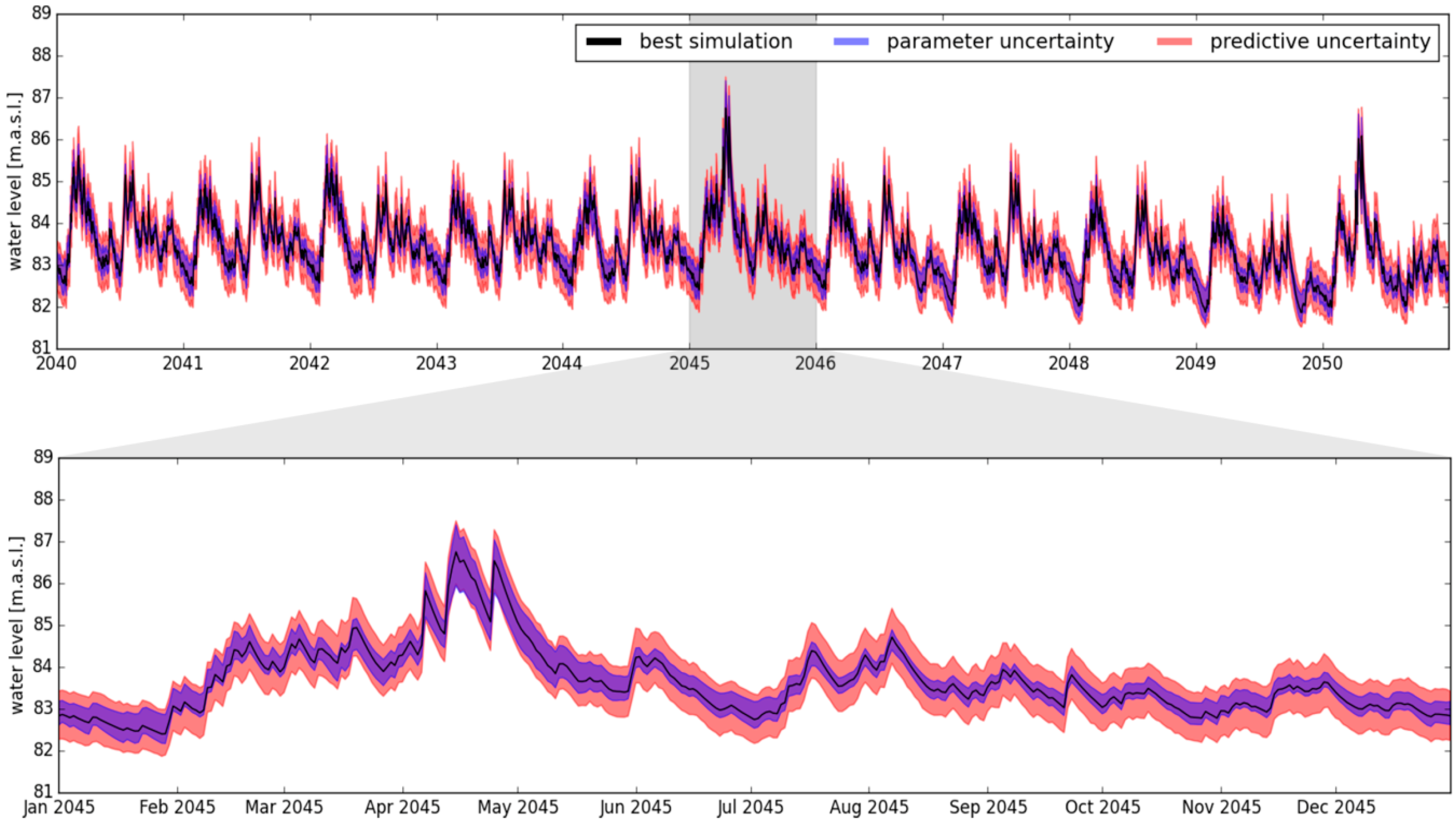
The ranges of the uncertainty bands for the two uncertainty methods addressed here, i.e., HBV parameter and predictive uncertainty, are almost the same for the GCMs and RCPs during both the mid- and the end-century (Table 1; an exemplary time sequence is given in the Appendix A, Figure A3). We observed that the uncertainty band of the predictive uncertainty is about 50% larger than that of the parameter uncertainty. The mean range of parameter uncertainty between the 5th and 95th percentiles was 0.85 m for the past and between 0.35 m and 0.56 m for the future period. In contrast, the mean range for the predictive uncertainty increases from 1.16 m in the past period to 1.18 and to 1.35 m for the future periods.

3.2. Projection of Spatial Inundation

The projected water levels of HBV are used to run the surface water–groundwater model CMF to simulate spatially distributed water levels of the floodplain on daily time steps. We used two different indicators to characterize inundation: the number of inundation days per year (Figure 4) and the mean duration of inundation period (Figure 5).
For the mid-century and the MPI-ESM model, a decrease of four to ten inundation days per year compared to the past period is estimated considering all three RCPs. This is observed for almost the same sites (polygons) in all three RCPs. Results for the HadGEM model are different. Some sites are estimated to have less inundation days on average, while the majority of polygons with changes depict an increase. Furthermore, the number of sites with projected changes of inundation days is higher for the HadGEM model than for the MPI-ESM model. Comparing the mid- to end-century projection, the number of polygons with a changing amount of inundation days at the end-century is less than in the mid-century for both GCMs. The magnitude of changes of inundation days towards the end-century is almost the same for the MPI-ESM model and the RCP 4.5 of the HadGEM model. Under the HadGEM, some sites change from an increase to decrease of inundation days during the mid-century to the end-century, respectively. For the mid-century, the spatial extension of changes in inundation days under HadGEM are decreasing with increasing RCPs, whereas for the end-century, the the spatial extension increases with increasing RCP. For MPI-ESM, the spatial distribution of polygons with changes in inundation days is nearly the same across all RCPs, and even the magnitude of the changes is similar. Overall, the differences between the RCPs are smaller compared to the differences between the GCMs.
On the whole, the projections for the duration of the mean annual inundation period (in days) (Figure 5) show the same pattern as for the annual number of inundation days (Figure 4). The spatial extensions of changes in the MPI-ESM model are almost the same for all RCPs within both time periods. Under the HadGEM GCM, a broader variance in the sites affected by the changes can be seen for the three RCPs. The number of sites with projected changes and the intensity of changes are higher for HadGEM than for MPI-ESM. However, some sites demonstrate a contrasting change (increase/decrease) between the RCPs under HadGEM, whereas under MPI-ESM the tendency of all sites to change is almost the same between the RCPs.

3.3. Uncertainty of Projections

This section shows the projected annual inundation days and their differences in projections, considering various sources of differences within the projections, i.e., differences caused by the GCMs, the RCPs and the parameter and predictive uncertainty of HBV.
Figure 6 represents the difference of the annual inundation days clustered by the sources causing the differences (GCMs, RCPs, and HBV). The difference is calculated as the variation between the two components (for GCM: HadGEM and MPI-ESM, for RCP: RCP 2.8 and RCP 8.5, and for HBV: predictive and parameter uncertainty). For each source, we estimated the mean annual inundation days by averaging the mean annual inundation days of each possible combination with the other components of sources. The absolute difference between the two components of the source is then stated as quantitative uncertainty (for the corresponding source).
The magnitude of the differences is higher overall when results are clustered based on the considered GCMs or input-driving data for the groundwater–surface water model from the HBV model compared to the differences introduced by the RCPs. On the other hand, the spatial extension of differences is greater for the GCMs and RCPs than for the differences caused by HBV for the mid-century, and it is a bit larger for the GCM and HBV than for the RCP for the end-century. All in all, the spatial extension of differences is much larger for the mid-century than for the end-century for the GCM and RCP. For the HBV source, the spatial extension is nearly the same for the mid- and end-century. The mean difference for the mid-century is 12.6, 3.8, and 20.0 days for the GCM, RCP, and HBV source, respectively (end-century: 22.1 days (GCM), 5.2 days (RCP), and 21.5 days (HBV)).
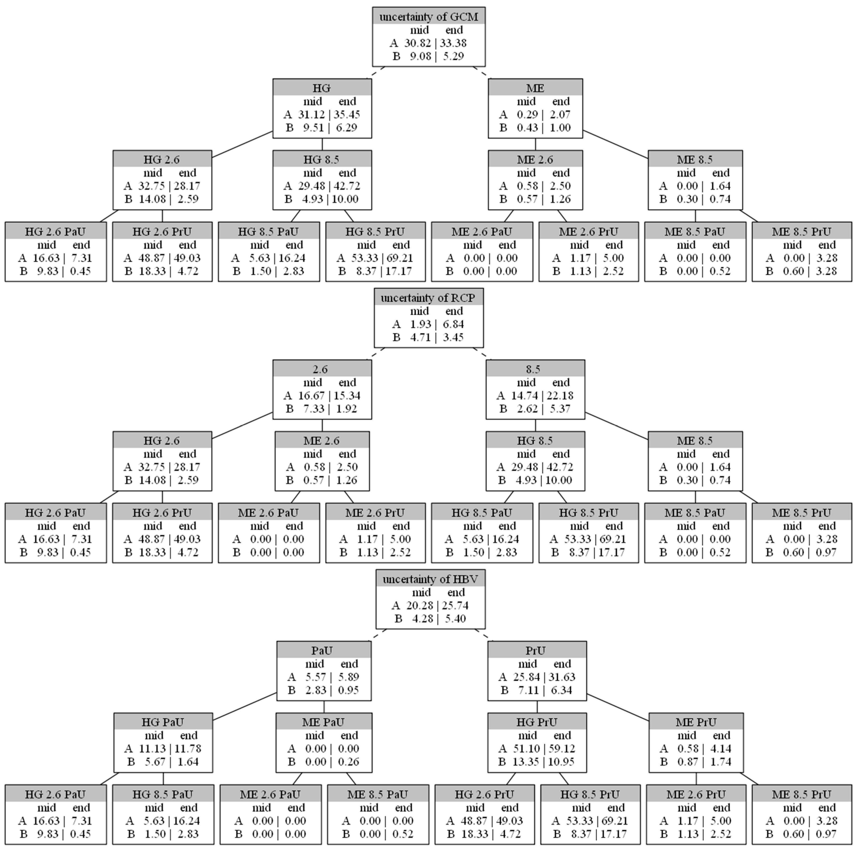
As an example, for the calculated difference of each polygon (Figure 6), the derivation for two polygons (marked as A and B) is shown in Figure A1 in the form of a tree diagram. Polygon A shows a large difference between the mean annual inundation days between the two GCMs (mid-century: 30.8 days, end-century: 33.4 days) as well between the different water levels under the HBV, representing the parameter and predictive uncertainties (mid-century: 20.3 days, end-century: 25.7 days), whereas the differences between the RCPs is rather small (mid-century: 1.9 days, end-century: 6.8 days). For polygon B, the difference arising from the RCPs and the water levels from HBV are nearly the same for the mid-century (RCP: 4.7 days, HBV mid-century: 4.3 days), whereas the difference arising from the GCM is about double (9.1 days). For the end-century, the difference between the GCMs and between the parameter and predictive uncertainty of the HBV model are nearly the same (GCM: 5.3, HBV: 5.4 days), and the differences between the RCPs are lower (3.5 days).
Additionally, our findings show that it is necessary to consider as many uncertainties as possible within a modeling procedure, including several models and steps. For example, a difference in the range of mean annual inundation days can be seen when considering the uncertainty introduced by the parameter and predictive uncertainties in the HBV model under the two GCMs. The mean annual inundation days under the HadGEM model are predominantly higher than under the MPI-ESM model (Figure A1, bottom. Reported as HadGEM model, Parameter Uncertainty (HG PaU) vs. MPI-ESM model, Parameter uncertainty (ME PaU) and HadGEM model, predictive uncertainty (HG PrU) vs. MPI-ESM model, predictive uncertainty (ME PrU)).

4. Discussion

Our HBV model of the Rhine River showed satisfactory results for the calibration and validation periods, and it was able to reproduce peak flow as well as low flow conditions very well (Appendix A, Figure A2). The same results have also been observed in other applications of the HBV model for the Rhine River (e.g., [43]). We found that the water level of the Rhine River is the primary driving variable for the groundwater–surface water model, as the Rhine River is known to be directly connected with the groundwater of the floodplain and is mainly responsible for the groundwater level changes [34].
A similar trend of the water level changes for the best simulation of the HBV model was found for both climate scenarios and the different concentration pathways (differentiated by the month of the year, Figure 3). The mean range of the uncertainty band for the different projections (Table 1) is smaller for the parameter uncertainty (0.35–0.56 m) than for the predictive uncertainty (1.18–1.35 m). This is an indication for other prominent uncertainty sources for the model (e.g., model context, structure or forcing data), except that of the parameters [64]. The differences in the mean range of the water level between the GCMs and RCPs are very small (predictive uncertainty: <0.10 m, parameter uncertainty: <0.17 m). In contrast, the inundation characteristics (annual inundation days and average annual inundation period) show large differences between the climate projections. While HadGEM indicates an increase in annual inundation days over large areas, MPI-ESM actually projects a decrease at some sites (Figure 4 and Figure 5).
To quantify the magnitude of all three sources (GCMs, RCPs, and the input driving data for CMF from the HBV model), causing differences in the mean annual inundation days, we averaged the annual inundation days of all possible model combinations for each component of each source (Figure 6). With this information, we could emphasize that our results are very sensitive to the used GCM. In addition, we showed that the input driving data from the HBV model have an important influence as well on the inundation of the study area. For both components of input driving data (predictive and parameter uncertainty), the annual inundation days are much larger under HadGEM. The mean seasonal amount of precipitation for the two GCMs already indicates different trends (Appendix A, Table A2). Whereas the HadGEM model shows a larger increase in autumn precipitation (+25.26%) than in spring precipitation (+2.47%), the MPI model shows a larger increase in spring precipitation (+24.47%) than in autumn precipitation (−3.10%). For winter and summer, both models show the same trend (increasing in winter (HadGEM: +33.85%, MPI-ESM: +47.95%) and decreasing in summer (HadGEM: -13.05%, MPI-ESM: −18.68%)). Following this, under the HadGEM, the mean simulated water level by HBV shows the largest increase (+1.23%) in summer and autumn. Under the MPI-ESM model, the increases in the water levels in summer and autumn are not as high (+0.54%) as under the HadGEM model (Appendix A, Table A3). This shows that it is necessary to consider the cascading uncertainty, because the final uncertainty is dependent on the uncertainty sources of the driving variables from the previously-applied model, as already depicted by other authors [65].
Similar to our study, Her et al. [66] evaluated the contribution of uncertainties contained in multi-GCM and multi-parameter ensembles. They considered one hydrological model (ABCD) and concluded that the significance of GCM and hydrological parameter selection varies, depending on the hydrological components. For instance, they showed that streamflow is affected by the uncertainty of GCMs and that the uncertainty of parameter ensembles influences groundwater projections. This is partially consistent with our results: the GCMs and the uncertainty of the water level projections of the Rhine River (including parameter uncertainty of HBV) have a large influence on the inundation characteristics. However, our results also indicate that the GCMs are a single, dominating source for different results when neglecting any further possible sources, e.g., the uncertainty of the discharge of the Rhine River (shown in the results of the spatial distribution of inundation days in Figure 3). Chen et al. [67] ranked several uncertainty sources (GCM, emission scenarios, GCM initial conditions, downscaling techniques, hydrological model, and hydrological model parameters) for seven hydrological criteria (annual/seasonal discharge, time to start/peak/end of the flood). GCMs were the largest source of uncertainty for all criteria, which aligns with our results.
Our applied climate change projections show many varying impacts to the floodplain of the Rhine River, from an increasing to decreasing trend of annual inundation days per year, from large to rather small spatial changes in inundation characteristics, and from large to small differences. Only for a small area (3.8 km2 in the southwest region of the study area, close to the cut-off meander of the Rhine River) no inundation is simulated under any projection.
Choosing a different RCP means choosing a different future, with either higher or lower concentration pathways; hence, the difference of the two is rather representative of the benefits of mitigation. Strangely enough, our results, especially under the MPI-ESM model, do not really suggest there is much benefit in mitigation. The difference in the rather optimistic RCP 2.6 and the rather pessimistic RCP 8.5 is rather small compared to the differences arising from the selection of the GCM and the underlying uncertainties arising from the hydrological modeling. The future predictions of the Rhine river remains very uncertain compared to other large river basins world-wide [68].
On the whole, changes in potential habitats on the floodplain are likely, but the extent and the direction of the changes are unclear due to the uncertainties induced by the models and the climate change scenarios. Nevertheless, the estimated changes in inundations would have large effects for species living in these areas, as we identified relevant changes in inundation duration and frequency for as soon as the mid-century period. Not included in our study, but equally important, are land-use modifications, e.g., by humans, political economics or structures. Land use changes, such as forest degradation or fertilization, can lead directly or indirectly through changes of the inundation patterns and water availability to changes in biodiversity and habitat availability. For this reason, such sites should be treated with caution when it comes to the management of natural resources, restoration measures, or implementation of biodiversity protections schemes [9,69].

5. Conclusions

The work carried out here presents a methodological approach to evaluating the impact of climate change on the inundation characteristics on a typical floodplain of one of Germany’s largest rivers. We considered different climate models, emission scenarios, and Bayesian methods to assess the uncertainty of our model chain. By linking an established rainfall–runoff model with a parsimonious surface water–groundwater model, we are able to project the future habitat conditions of floodplains.
The results presented should be interpreted as trends and not as an accurate quantitative prediction, particularly regarding the uncertainties related to the GCMs. We recommend the consideration of a larger ensemble of GCMs to better constrain the potential effects of climate change in these ecosystems.
The projected shift of inundation patterns and their extent will have consequences for habitat availability and species distribution, which will occur during the course of climate change. Such information is especially valuable for the protection of endangered species and for the long-term planning and success of renaturation projects in biodiversity-rich floodplains. After linking ecological habitat models to our modeling chain, the next step forward will be to project habitat distribution and quality under climate change.

Author Contributions

Conceptualization, N.M.; Methodology, N.M., P.K., T.H., A.C.; Software, N.M., P.K., T.H., A.C.; Validation, N.M.; Formal Analysis, N.M.; Investigation, N.M.; Resources, N.M., P.K., T.H., A.C., L.B.; Writing-Original Draft Preparation, N.M.; Writing-Review & Editing, T.H., A.C., L.B., P.K.; Visualization, N.M.; Supervision, T.H., P.K., L.B.; Project Administration, P.K.; Funding Acquisition, P.K., L.B.

Funding

This research was funded by the Deutsche Bundesstiftung Umwelt DBU (project 31612–33/0; www.dbu.de). Tobias Houska and Alejandro Chamorro acknowledge funding through the DFG grants BR2238/13-1 (Uncertainty of predicted hydro-biogeochemical fluxes and trace gas emissions on the landscape scale under climate and land use change) and BR2238/5-2 (Ensemble projections of hydro-biogeochemical fluxes under climate change), respectively.

Acknowledgments

The climate data used are available from Germany’s national meteorological service (Deutscher Wetterdienst (DWD), http://www.dwd.de/cdc; ftp://ftp-cdc.dwd.de/pub/CDC). Daily water levels from the Nierstein gauging station are available from the Federal Waterways and Shipping Authority (Wasser und Schifffahrtsverwaltung des Bundes (WSV)) and provided by the Federal Institute of Hydrology (Bundesanstalt für Gewässerkunde (BfG)). Groundwater levels are provided by the Hessian State Office for Conservation, Environment and Geology (Hessisches Landesamt für Naturschutz, Umwelt und Geologie (HLNUG)). Precipitation and temperature data for the GCMs are taken from the IPCC data distribution center (http://cera-www.dkrz.de).

Conflicts of Interest

The authors declare no conflicts of interest. The funders had no role in the design of the study; in the collection, analyses, or interpretation of data; in the writing of the manuscript, and in the decision to publish the results.

Appendix A

Figure A1. Example of the quantification of differences in the mean annual inundation days for the polygons A and B (Figure 3) for the mid-century and the end-century, represented in the form of tree diagrams. Each node at the bottom represents the mean annual inundation days of the two polygons (A and B) of a simulation. The nodes one and two levels higher depict the mean of the two lower nodes. Only the node in the top depicts the difference between the two lower nodes (depicted by dashed lines); i.e., the top node indicates the difference between the mean annual inundation days and represents the quantitative uncertainty. Abbreviations used: HG = HadGEM, ME = MPI-ESM, 2.6 = RCP 2.6, 8.5 = RCP 8.5, PrU = predictive uncertainty, PaU = parameter uncertainty.
Water 10 00809 g0a1
Table A1. HBV model parameters, their meaning, range for calibration and value for best performing parameter set.
ParameterDescriptionUnitLower Bound–Upper BoundBest Parameter Set
CEPotential Evapotranspiration model parameter-0.01–0.20.09
ThetaActual evapotranspiration coefficient-0.8–1.51.00
TTThreshold melting Temperature°C−0.98–20.43
CmeltSow melting parameter-0.2–2.01.10
FCField capacitymm40–250207.56
BetaModel parameter-1–51.00
PWPPermanent wilting pointmm40–250159.82
LDepth of upper reservoirmm1–10041.50
K1Surface flow storage constant1/d10–80025.27
K2Interflow storage constant1/d10–85035.85
KZPercolation storage constant1/d10–980178.53
K3Baseflow storage constant1/d10–1000353.30
Figure A2. Performance of the HBV model, shown for the best performing parameter set for the years 2001 to 2013 (top) and for the year 1007 with the parameter and the predictive uncertainty band (bottom).
Water 10 00809 g0a2
Figure A3. Projected water levels of the Rhine river and the associated uncertainty bands (parameter and predictive uncertainty), exemplarily shown for the years 2040 to 2050 (top) and for the year 2045 (bottom).
Water 10 00809 g0a3
Table A2. Changes in the amount of precipitation for different seasons for the weather station in Darmstadt. The change is given in percentage compared to the observed period for the historical data (from the GCMs) and compared to the historical period of the GCM for the RCPs. Data are downscaled by using quantile mapping. The arrows indicate the direction and the magnitude of the trend.
GCM WinterSpringSummerAutumn
2000–2005 observed171.50 mm183.88 mm197.35 mm196.72 mm
HadGEMhistorical−8.53% −0.17% −11.75% −0.27%
MPI-ESMMPI-ESM−19.80% −5.06% −3.95% 0.06%
2021–2050HadGemRCP 2.614.73% −0.05% −11.42% 17.87%
RCP 4.541.21% 4.62% −3.77% 24.09%
RCP 8.524.36% 7.29% −9.52% 30.91%
MPIRCP 2.649.65% 28.51% −7.62% 5.53%
RCP 4.548.44% 33.52% −8.87% −4.52%
RCP 8.541.14% 19.12% −15.60% 1.64%
2021–2050HadGemRCP 2.634.57% 6.55% 3.68% 15.00%
RCP 4.532.23% −5.90% −17.52% 35.25%
RCP 8.555.99% 2.30% −39.73% 28.44%
MPIRCP 2.650.70% 17.54% −12.67% 0.37%
RCP 4.546.24% 23.80% −23.67% −13.05%
RCP 8.551.50% 24.30% −43.64% −8.56%
Table A3. Changes in the mean water level at the gauging station Mainz (observed and simulated with HBV) for different seasons. The change is given in percentage compared to the observed period for the historical data from the GCMs) and compared to the historical period of the GCM for the RCP’s. The arrows indicate the direction and the magnitude of the trend.
GCM WinterSpringSummerAutumn
2000–2005 observed83.12 m83.34 m82.99 m82.76 m
HadGEMhistorical−0.31% 0.27% −0.05% 0.11%
MPI-ESMMPI-ESM−0.19% −0.13% 0.04% 0.32%
2021–2050HadGemRCP 2.60.68% 0.30% 1.22% 1.21%
RCP 4.50.81% 0.41% 1.33% 1.30%
RCP 8.50.66% 0.29% 1.21% 1.21%
MPIRCP 2.60.25% 0.39% 0.76% 0.64%
RCP 4.50.18% 0.49% 0.75% 0.59%
RCP 8.50.11% 0.35% 0.74% 0.54%
2021–2050HadGemRCP 2.60.64% 0.26% 1.22% 1.18%
RCP 4.50.74% 0.31% 1.24% 1.27%
RCP 8.50.72% 0.25% 1.20% 1.19%
MPIRCP 2.60.22% 0.39% 0.78% 0.61%
RCP 4.50.07% 0.27% 0.54% 0.35%
RCP 8.50.02% 0.28% 0.17% 0.08%

References

  1. Hayashi, M.; Rosenberry, D.O. Effects of Ground Water Exchange on the Hydrology and Ecology of Surface Water. Ground Water 2002, 40, 309–316. [Google Scholar] [CrossRef] [PubMed]
  2. Maltby, E.; Barker, T. (Eds.) The Wetlands Handbook; Wiley-Blackwell: Oxford, UK, 2009; ISBN 978-1-4443-1581-3. [Google Scholar]
  3. Van Eck, W.H.J.M.; Van De Steeg, H.M.; Blom, C.W.P.M.; De Kroon, H. Is tolerance to summer flooding correlated with distribution patterns in river floodplains? A comparative study of 20 terrestrial grassland species. Oikos 2004, 107, 393–405. [Google Scholar] [CrossRef]
  4. Woodcock, B.A.; Mann, D.J.; Mirieless, C.; McGavin, G.C.; McDonald, A.W. Re-creation of a lowland flood-plain meadow. J. Insect Conserv. 2005, 9, 207–218. [Google Scholar] [CrossRef]
  5. Krause, S.; Bronstert, A.; Zehe, E. Groundwater-surface water interactions in a North German lowland floodplain—Implications for the river discharge dynamics and riparian water balance. J. Hydrol. 2007, 347, 404–417. [Google Scholar] [CrossRef]
  6. Taylor, R.G.; Scanlon, B.; Döll, P.; Rodell, M.; van Beek, R.; Wada, Y.; Longuevergne, L.; Leblanc, M.; Famiglietti, J.S.; Edmunds, M.; et al. Ground water and climate change. Nat. Clim. Chang. 2012, 3, 322–329. [Google Scholar] [CrossRef] [Green Version]
  7. Van Roosmalen, L.; Christensen, B.S.B.; Sonnenborg, T.O. Regional Differences in Climate Change Impacts on Groundwater and Stream Discharge in Denmark. Vadose Zone J. 2007, 6, 554–571. [Google Scholar] [CrossRef]
  8. Tockner, K.; Stanford, J.A. Riverine flood plains: Present state and future trends. Environ. Conserv. 2002, 29, 308–330. [Google Scholar] [CrossRef]
  9. Opperman, J.J.; Luster, R.; McKenney, B.A.; Roberts, M.; Meadows, A.W. Ecologically Functional Floodplains: Connectivity, Flow Regime, and Scale. J. Am. Water Resour. Assoc. 2010, 46, 211–226. [Google Scholar] [CrossRef]
  10. Capon, S.J.; Chambers, L.E.; Nally, R.M.; Naiman, R.J.; Davies, P.; Marshall, N.; Pittock, J.; Reid, M.; Capon, T.; Douglas, M.; et al. Riparian Ecosystems in the 21st Century: Hotspots for Climate Change Adaptation? Ecosystems 2013, 16, 359–381. [Google Scholar] [CrossRef]
  11. Demirel, M.C.; Booij, M.J.; Hoekstra, A.Y. Impacts of climate change on the seasonality of low flows in 134 catchments in the River Rhine basin using an ensemble of bias-corrected regional climate simulations. Hydrol. Earth Syst. Sci. 2013, 17, 4241–4257. [Google Scholar] [CrossRef] [Green Version]
  12. Dokulil, M. Impact of climate warming on European inland waters. Inland Waters 2014, 4, 27–40. [Google Scholar] [CrossRef]
  13. Middelkoop, H.; Daamen, K.; Gellens, D.; Grabs, W.; Kwadijk, J.C.; Lang, H.; Parmet, B.W.; Schädler, B.; Schulla, J.; Wilke, K. Impact of climate change on hydrological regimes and water resources management in the Rhine basin. Clim. Chang. 2001, 49, 105–128. [Google Scholar] [CrossRef]
  14. Herron, N.; Davis, R.; Jones, R. The effects of large-scale afforestation and climate change on water allocation in the Macquarie River catchment, NSW, Australia. J. Environ. Manag. 2002, 65, 369–381. [Google Scholar] [CrossRef]
  15. Mortsch, L.D. Assessing the impact of climate change on the Great Lakes shoreline wetlands. Clim. Chang. 1998, 40, 391–416. [Google Scholar] [CrossRef]
  16. Sorenson, L.G.; Goldberg, R.; Root, T.L.; Anderson, M.G. Potential Effects of Global Warming on Waterfowl Populations Breeding in the Northern Great Plains. Clim. Chang. 1998, 40, 343–369. [Google Scholar] [CrossRef]
  17. Thompson, J.R.; Gavin, H.; Refsgaard, A.; Refstrup Sørenson, H.; Gowing, D.J. Modelling the hydrological impacts of climate change on UK lowland wet grassland. Wetlands Ecol. Manag. 2009, 17, 503–523. [Google Scholar] [CrossRef]
  18. Opperman, J.J.; Galloway, G.E.; Fargione, J.; Mount, J.F.; Richter, B.D.; Secchi, S. Sustainable floodplains through large-scale reconnection to rivers. Science 2009, 326, 1487–1488. [Google Scholar] [CrossRef] [PubMed]
  19. Furman, A. Modeling Coupled Surface–Subsurface Flow Processes. Vadose Zone J. 2008, 7, 741. [Google Scholar] [CrossRef]
  20. Refsgaard, J.C.; Sørensen, H.R.; Mucha, I.; Rodak, D.; Hlavaty, Z.; Bansky, L.; Klucovska, J.; Topolska, J.; Takac, J.; Kosc, V.; et al. An Integrated Model for the Danubian Lowland—Methodology and Applications. Water Resour. Manag. 1998, 12, 433–465. [Google Scholar] [CrossRef]
  21. Alaghmand, S.; Beecham, S.; Woods, J.A.; Holland, K.L.; Jolly, I.D.; Hassanli, A.; Nouri, H. Quantifying the impacts of artificial flooding as a salt interception measure on a river-floodplain interaction in a semi-arid saline floodplain. Environ. Model. Softw. 2016, 79, 167–183. [Google Scholar] [CrossRef]
  22. House, A.R.; Thompson, J.R.; Acreman, M.C. Projecting impacts of climate change on hydrological conditions and biotic responses in a chalk valley riparian wetland. J. Hydrol. 2016, 534, 178–192. [Google Scholar] [CrossRef]
  23. Karim, F.; Petheram, C.; Marvanek, S.; Ticehurst, C.; Wallace, J.; Hasan, M. Impact of climate change on floodplain inundation and hydrological connectivity between wetlands and rivers in a tropical river catchment. Hydrol. Process. 2016, 30, 1574–1593. [Google Scholar] [CrossRef]
  24. Bredehoeft, J. The conceptualization model problem? Hydrogeol. J. 2005, 13, 37–46. [Google Scholar] [CrossRef]
  25. Kay, A.L.; Davies, H.N.; Bell, V.A.; Jones, R.G. Comparison of uncertainty sources for climate change impacts. Clim. Chang. 2009, 92, 41–63. [Google Scholar] [CrossRef] [Green Version]
  26. Refsgaard, J.C.; van der Sluijs, J.P.; Brown, J.; van der Keur, P. A framework for dealing with uncertainty due to model structure error. Adv. Water Resour. 2006, 29, 1586–1597. [Google Scholar] [CrossRef] [Green Version]
  27. Teng, J.; Vaze, J.; Chiew, F.H.S.; Wang, B.; Perraud, J.-M. Estimating the Relative Uncertainties Sourced from GCMs and Hydrological Models in Modeling Climate Change Impact on Runoff. J. Hydrometeorol. 2012, 13, 122–139. [Google Scholar] [CrossRef]
  28. Wilby, R.L. Uncertainty in water resource model parameters used for climate change impact assessment. Hydrol. Processes 2005, 19, 3201–3219. [Google Scholar] [CrossRef]
  29. Wilby, R.L.; Whitehead, P.G.; Wade, A.J.; Butterfield, D.; Davis, R.J.; Watts, G. Integrated modelling of climate change impacts on water resources and quality in a lowland catchment. J. Hydrol. 2006, 330, 204–220. [Google Scholar] [CrossRef]
  30. McMillan, H.K.; Brasington, J. End-to-end flood risk assessment. Water Resour. Res. 2008, 44, 295. [Google Scholar] [CrossRef]
  31. Pappenberger, F.; Beven, K.J.; Hunter, N.M.; Bates, P.D.; Gouweleeuw, B.T.; Thielen, J.; Roo, A.P.J. Cascading model uncertainty from medium range weather forecasts (10 days) through a rainfall-runoff model to flood inundation predictions within the European Flood Forecasting System (EFFS). Hydrol. Earth Syst. Sci. 2005, 9, 381–393. [Google Scholar] [CrossRef] [Green Version]
  32. Sorribas, M.V.; Paiva, R.C.D.; Melack, J.M.; Bravo, J.M.; Jones, C.; Carvalho, L.; Beighley, E.; Forsberg, B.; Costa, M.H. Projections of climate change effects on discharge and inundation in the Amazon basin. Clim. Chang. 2016, 136, 555–570. [Google Scholar] [CrossRef]
  33. Barron, O.; Silberstein, R.; Ali, R.; Donohue, R.; McFarlane, D.J.; Davies, P.; Hodgson, G.; Smart, N.; Donn, M. Climate change effects on water-dependent ecosystems in south-western Australia. J. Hydrol. 2012, 434–435, 95–109. [Google Scholar] [CrossRef]
  34. Maier, N.; Breuer, L.; Kraft, P. Prediction and uncertainty analysis of a parsimonious floodplain surface water–groundwater interaction model. Water Resour. Res. 2017. [Google Scholar] [CrossRef]
  35. Kraft, P.; Vaché, K.B.; Frede, H.-G.; Breuer, L. CMF: A Hydrological Programming Language Extension For Integrated Catchment Models. Environ. Model. Softw. 2011, 26, 828–830. [Google Scholar] [CrossRef]
  36. Kraft, P. cmf-Catchment Modelling Framework. Available online: http://fb09-pasig.umwelt.uni-giessen.de/cmf (accessed on 18 June 2018).
  37. Qu, Y.; Duffy, C.J. A semidiscrete finite volume formulation for multiprocess watershed simulation. Water Resour. Res. 2007, 43. [Google Scholar] [CrossRef] [Green Version]
  38. Allen, R.G.; Pereira, L.S.; Raes, D.; Smith, M. Crop Evapotranspiration; FAO Irrigation and Drainage Paper; FAO: Rome, Italy, 1998; Volume 56, ISBN 92-5-104219-5. [Google Scholar]
  39. Bergström, S. The HBV model. In Computer Models of Watershed Hydrology; Singh, V.P., Ed.; Water Resources Publications: Highlands Ranch, CO, USA, 1995; pp. 443–476. ISBN 978-0-918334-91-6. [Google Scholar]
  40. Lindström, G.; Johansson, B.; Persson, M.; Gardelin, M.; Bergström, S. Development and test of the distributed HBV-96 hydrological model. J. Hydrol. 1997, 201, 272–288. [Google Scholar] [CrossRef]
  41. Bárdossy, A.; Singh, S.K. Robust estimation of hydrological model parameters. Hydrol. Earth Syst. Sci. 2008, 12, 1273–1283. [Google Scholar] [CrossRef] [Green Version]
  42. Huang, S.; Kumar, R.; Flörke, M.; Yang, T.; Hundecha, Y.; Kraft, P.; Gao, C.; Gelfan, A.; Liersch, S.; Lobanova, A.; et al. Evaluation of an ensemble of regional hydrological models in 12 large-scale river basins worldwide. Clim. Chang. 2017, 141, 381–397. [Google Scholar] [CrossRef]
  43. Te Linde, A.H.; Aerts, J.C.J.H.; Hurkmans, R.T.W.L.; Eberle, M. Comparing model performance of two rainfall-runoff models in the Rhine basin using different atmospheric forcing data sets. Hydrol. Earth Syst. Sci. 2008, 12, 943–957. [Google Scholar] [CrossRef] [Green Version]
  44. Vetter, T.; Huang, S.; Aich, V.; Yang, T.; Wang, X.; Krysanova, V.; Hattermann, F. Multi-model climate impact assessment and intercomparison for three large-scale river basins on three continents. Earth Syst. Dyn. 2015, 6, 17–43. [Google Scholar] [CrossRef] [Green Version]
  45. Beven, K.; Binley, A. The future of distributed models: Model calibration and uncertainty prediction. Hydrol. Processes 1992, 6, 279–298. [Google Scholar] [CrossRef]
  46. Houska, T.; Kraft, P.; Chamorro-Chavez, A.; Breuer, L. SPOTting Model Parameters Using a Ready-Made Python Package. PLoS ONE 2015, 10, e0145180. [Google Scholar] [CrossRef] [PubMed]
  47. Nash, J.E.; Sutcliffe, J.V. River flow forecasting through conceptual models part I—A discussion of principles. J. Hydrol. 1970, 10, 282–290. [Google Scholar] [CrossRef]
  48. McInerney, D.; Thyer, M.; Kavetski, D.; Lerat, J.; Kuczera, G. Improving probabilistic prediction of daily streamflow by identifying Pareto optimal approaches for modeling heteroscedastic residual errors. Water Resour. Res. 2017, 53, 2199–2239. [Google Scholar] [CrossRef]
  49. Box, G.E.P.; Cox, D.R. An Analysis of Transformations-Revisited. J. Am. Statist. Assoc. 1982, 77, 177–182. [Google Scholar] [CrossRef]
  50. Taylor, K.E.; Stouffer, R.J.; Meehl, G.A. An Overview of CMIP5 and the Experiment Design. Bull. Am. Meteorol. Soc. 2012, 93, 485–498. [Google Scholar] [CrossRef] [Green Version]
  51. McSweeney, C.F.; Jones, R.G.; Lee, R.W.; Rowell, D.P. Selecting CMIP5 GCMs for downscaling over multiple regions. Clim. Dyn. 2015, 44, 3237–3260. [Google Scholar] [CrossRef]
  52. Brands, S.; Herrera, S.; Fernández, J.; Gutiérrez, J.M. How well do CMIP5 Earth System Models simulate present climate conditions in Europe and Africa? Clim. Dyn. 2013, 41, 803–817. [Google Scholar] [CrossRef] [Green Version]
  53. Keuler, K.; Radtke, K.; Kotlarski, S.; Lüthi, D. Regional climate change over Europe in COSMO-CLM: Influence of emission scenario and driving global model. Meteorol. Z. 2016, 25, 121–136. [Google Scholar] [CrossRef]
  54. Zubler, E.M.; Fischer, A.M.; Fröb, F.; Liniger, M.A. Climate change signals of CMIP5 general circulation models over the Alps—Impact of model selection. Int. J. Climatol. 2016, 36, 3088–3104. [Google Scholar] [CrossRef]
  55. Maraun, D.; Wetterhall, F.; Ireson, A.M.; Chandler, R.E.; Kendon, E.J.; Widmann, M.; Brienen, S.; Rust, H.W.; Sauter, T.; Themeßl, M.; et al. Precipitation downscaling under climate change. Rev. Geophys. 2010, 48, 219. [Google Scholar] [CrossRef]
  56. Themeßl, M.J.; Gobiet, A.; Leuprecht, A. Empirical-statistical downscaling and error correction of daily precipitation from regional climate models. Int. J. Climatol. 2011, 31, 1530–1544. [Google Scholar] [CrossRef]
  57. Prudhomme, C.; Davies, H. Assessing uncertainties in climate change impact analyses on the river flow regimes in the UK. Part 2. Clim. Chang. 2009, 93, 197–222. [Google Scholar] [CrossRef]
  58. Quintana Seguí, P.; Ribes, A.; Martin, E.; Habets, F.; Boé, J. Comparison of three downscaling methods in simulating the impact of climate change on the hydrology of Mediterranean basins. J. Hydrol. 2010, 383, 111–124. [Google Scholar] [CrossRef] [Green Version]
  59. Chen, J.; Brissette, F.P.; Chaumont, D.; Braun, M. Finding appropriate bias correction methods in downscaling precipitation for hydrologic impact studies over North America. Water Resour. Res. 2013, 49, 4187–4205. [Google Scholar] [CrossRef] [Green Version]
  60. Gudmundsson, L.; Bremnes, J.B.; Haugen, J.E.; Engen-Skaugen, T. Downscaling RCM precipitation to the station scale using statistical transformations—A comparison of methods. Hydrol. Earth Syst. Sci. 2012, 16, 3383–3390. [Google Scholar] [CrossRef]
  61. Teutschbein, C.; Seibert, J. Bias correction of regional climate model simulations for hydrological climate-change impact studies. J. Hydrol. 2012, 456–457, 12–29. [Google Scholar] [CrossRef]
  62. David, P.G. Changes in plant communities relative to hydrologic conditions in the Florida Everglades. Wetlands 1996, 16, 15–23. [Google Scholar] [CrossRef]
  63. Mathar, W.; Kleinebecker, T.; Hölzel, N.; Collins, B. Environmental variation as a key process of co-existence in flood-meadows. J. Veg. Sci. 2015, 26, 480–491. [Google Scholar] [CrossRef]
  64. Mockler, E.M.; Chun, K.P.; Sapriza-Azuri, G.; Bruen, M.; Wheater, H.S. Assessing the relative importance of parameter and forcing uncertainty and their interactions in conceptual hydrological model simulations. Adv. Water Resour. 2016, 97, 299–313. [Google Scholar] [CrossRef]
  65. Refsgaard, J.C.; Arnbjerg-Nielsen, K.; Drews, M.; Halsnæs, K.; Jeppesen, E.; Madsen, H.; Markandya, A.; Olesen, J.E.; Porter, J.R.; Christensen, J.H. The role of uncertainty in climate change adaptation strategies—A Danish water management example. Mitig. Adapt. Strateg. Glob. Chang. 2013, 18, 337–359. [Google Scholar] [CrossRef] [Green Version]
  66. Her, Y.; Yoo, S.-H.; Seong, C.; Jeong, J.; Cho, J.; Hwang, S. Comparison of uncertainty in multi-parameter and multi-model ensemble hydrologic analysis of climate change. Hydrol. Earth Syst. Sci. Discuss. 2016, 1–44. [Google Scholar] [CrossRef]
  67. Chen, J.; Brissette, F.P.; Poulin, A.; Leconte, R. Overall uncertainty study of the hydrological impacts of climate change for a Canadian watershed. Water Resour. Res. 2011, 47, 176. [Google Scholar] [CrossRef]
  68. Pechlivanidis, I.G.; Arheimer, B.; Donnelly, C.; Hundecha, Y.; Huang, S.; Aich, V.; Samaniego, L.; Eisner, S.; Shi, P. Analysis of hydrological extremes at different hydro-climatic regimes under present and future conditions. Clim. Chang. 2017, 141, 467–481. [Google Scholar] [CrossRef]
  69. Eamus, D.; Froend, R.; Loomes, R.; Hose, G.; Murray, B. A functional methodology for determining the groundwater regime needed to maintain the health of groundwater-dependent vegetation. Aust. J. Bot. 2006, 54, 97–114. [Google Scholar] [CrossRef]
Figure 1. Geographic location of the study area (lower left), digital elevation of the larger nature reserve with the study area (middle), and the setup for the surface water–groundwater model in the catchment modeling framework (CMF) (right). The irregular polygons are based on similar elevation and land use.
Water 10 00809 g001
Figure 2. Flowchart showing the steps within the model framework. The steps within the dotted box represent steps forced by historical data and steps within the dashed box represent future projections. Models are depicted by grey boxes.
Water 10 00809 g002
Figure 3. Monthly boxplots of HBV-simulated water levels of the Rhine using the best-performing model parameter sets for representative concentration pathway (RCP) 2.6 (bluish, top), RCP 4.5 (greenish, middle), RCP 8.5 (reddish, bottom) and for two different periods (top: mid-century 2021–2050, bottom: end-century 2071–2100). Black boxplots represent observations for the period 1990–2015. The linear trend of the water level change is given below each boxplot for the time from 1990 to 2015 (under black boxplots), from 2021 to 2050 (upper figure of each RCP group, under colored boxplots), and from 2071 to 2100 (lower figure of each RCP group, under colored boxplots). Points indicate no trend; upward arrows indicate an increasing trend and downward arrows a decreasing trend at the significance level of p < 0.05 based on the Mann–Kendall Test. For significant trends, the absolute change for the time period is given in meters.
Water 10 00809 g003
Figure 4. Spatial distribution of average inundation days (per year) for the mid-century (2021–2050) and end-century (2071–2100) compared to the past (2002–2015). Results are shown for the different combinations of GCMs and RCPs as the difference of inundation days for the future period minus those from the past. Results shown for the CMF model are forced by simulated water levels of the Rhine River, using the best-performing HBV parameter set for the calibration period.
Water 10 00809 g004
Figure 5. Spatial distribution of average inundation duration (days per year) for the mid-century (2021–2050) and end-century (2071–2100) compared to the past (2002–2015). Results are shown for the combinations of GCMs and RCPs as the difference of average inundation duration for the future period minus those from the past. Results shown for the CMF model are forced by simulated water levels of the Rhine River, using the best-performing HBV parameter set for the calibration period.
Water 10 00809 g005
Figure 6. Uncertainty of the annual inundation days per time period separated by the three sources of uncertainty: GCMs, RCPs, and the parameter and predictive uncertainty of the HBV model. Each component represents the mean of all possible combinations, whereas each combination indicates the average annual flooding days. The filling patterns depict the mean annual inundation days from all simulations. The top panels show results for the mid-century, bottom panels for the end-century conditions. (A,B) indicate sites that are specifically referred to in the text.
Water 10 00809 g006
Table 1. Mean uncertainty (i.e., range of the daily water levels, averaged over the time period) of the Rhine water level of the parameter and predictive uncertainty. GCM: general circulation model. RCP: Representative Concentration Pathways.
Time PeriodPastMid-CenturyEnd-Century
GCM model HadGEMMPI-ESMHadGEMMPI-ESM
RCP 2.64.58.52.64.58.52.64.58.52.64.58.5
Parameter uncertainty0.850.460.500.460.470.480.560.370.360.370.410.350.39
Predictive uncertainty1.161.321.341.351.181.321.351.241.251.271.211.221.26