1. Introduction
Simulation of monthly streamflow serves various purposes of water resources planning and management. Decadal simulation of streamflow provides years-ahead insight on the capacity, adequacy, and reliability of a reservoir based on the anthropogenic changes in runoff [
1,
2,
3]. Conceptual and physically based models of the watershed, for example, SWAT (Soil and Water Assessment Tool), VIC (Variable Infiltration Capacity Macroscale Hydrologic Model), and PIHM (Penn State Integrated Hydrologic Modeling System) remain a popular choice among water resources managers. Such a model has the potential to include every component of a hydrologic process (conceptual) or mathematically replicate the physical phenomenon. A review of few physically-based models is provided by Devi et al. [
4]. These models require a bunch of data sets that delineate hydro-geological characteristic of a basin.
Statistical and machine learning techniques for rainfall-runoff modeling, also known as empirical modeling, have received significant attention from the researchers particularly in cases where supporting input data for process-based models are limited [
5]. Further improvement and application of statistical and machine learning techniques remain popular among researchers, despite the fact that these models are often criticized as black box models [
6], ignoring the physical process. A simple rainfall-runoff model considers precipitation as the model input and days to the years-ahead prediction of the streamflow as the model output. Empirical approaches for streamflow simulation may vary from simple regression to sophisticated machine learning algorithms such as an artificial neural network (ANN). Sharma et al. [
7] proposed a method to generate synthetic streamflow sequences based on kernel estimates of the joint and conditional probability density. The study produces sequences that represent future scenarios assuming that future remains similar to the past. Random number generator was used by Hirsch [
8] to simulate the traces of normally distributed innovations. Following that, studies [
9,
10,
11] employed several random sampling algorithms for uncertainty analysis and comparison purposes of network design [
1]. Recent studies focused on developing copula-based methods for monthly streamflow simulations [
12,
13]. Shortridge et al. [
14] compared a machine learning algorithm with a statistical approach-multiple regression to simulate streamflow over five rivers of Ethiopia. On the machine learning side, support-vector machines [
15,
16], regression tree based approach [
5,
17], and ANN [
18,
19] were used for rainfall-runoff modeling.
The objective of the present study is to employ a state-of-the-art statistical approach, Bayesian regression with multivariate linear spline (BMLS), for decades-ahead monthly streamflow simulation. The approach, initially proposed by Holmes and Mullick [
20], incorporates Bayesian analysis of the piece-wise linear model. The piece-wise linear model is formed with basis functions that generalize the univariate spline to higher dimensions [
20]. BMLS builds a regression surface with spline bases which select the covariate interactions uniformly and make the orientations suitably in all possible directions so that the estimated model has joint posterior optimality. The posterior model space of randomly located splines is integrated to obtain the posterior distribution of the response variable, streamflow in our case. The model features enable a smooth mean regression surface (posterior) from non-smooth piecewise prior model space. BMLS could be advantageous over existing statistical approaches for streamflow modeling since BMLS can deal with a large number of covariates while eliminating the irrelevant ones. The approach is also considered to be spatially adaptive [
20].
The current study estimates the changes in future streamflow caused by climate change using BMLS. The study also examines the quality of general circulation models’ (GCM) outputs in simulating streamflow. The Coupled Model Intercomparison Project Phase 5 (CMIP5) introduced hindcast runs, in addition to the historical runs, where climate models are driven by initialized sea-surface temperature (SST) [
21]. Hindcast runs, also known as decadal predictions, provide climate simulations for 10 and/or 30 years. These runs are archived as decadal-80, decadal-90, etc. based on the year of SST initialization. Earlier studies found that hindcast runs have the potential of preserving the precipitation and temperature cross-correlation [
22] and of predicting long-lead ENSO (El Niño-Southern Oscillation) events [
23]. Current study forces BMLS with outputs from multiple hindcast and historical runs to understand the improvement in empirical streamflow simulation from the SST initialization.
Details on the dataset are presented in
Section 2.
Section 3 describes the BMLS model, experimental design and the test statistics used for the study. Results are presented in
Section 4 which is followed by the Discussion.
3. Methodology
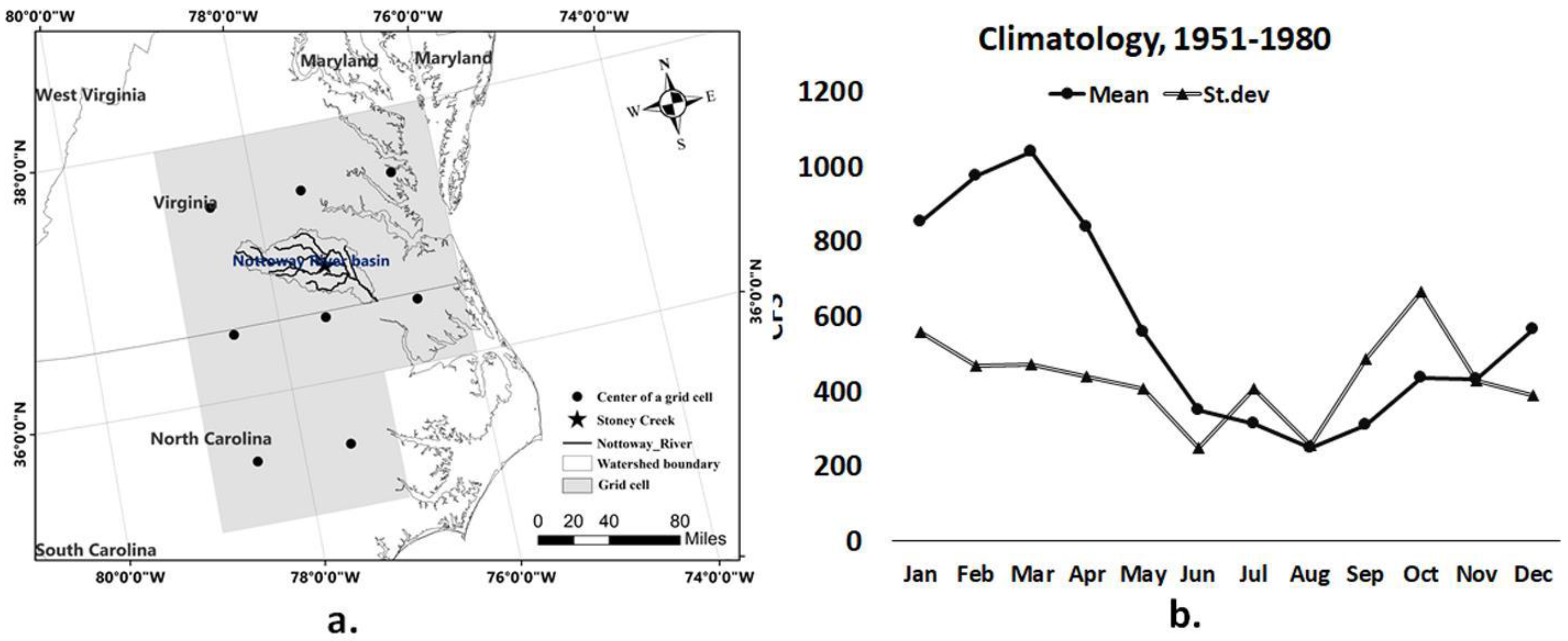
We use monthly temperature, precipitation and streamflow series obtained over a period of 360 months for the model-building purpose. The log-transformed streamflow is considered as the predictand. Let us denote St as the log-transformed streamflow, Ttk as the temperature and Ptk as the precipitation at the kth grid cell (k = 1, 2, …, 8) as observed on tth month (t = 1, 2, ..., 360).
There are eight variables on precipitation and eight variables on temperature. The proposed model is
The purpose of is to handle the temporal dependence of streamflow (defined as ). We assume has a known functional structure, for the current study, a seasonal autoregressive model (SAR) given by Φ, where Φ, where B is the lag operator, and s represents the period of the seasonal component. We incorporate the dependence of streamflow as a function of historical streamflow data of length h to ensure that the serial dependence of streamflow at lags of multiples of s are present as a source of variation. Here, s being the period of the seasonal components is necessarily the number of observations that make up a seasonal cycle. From the periodogram, autocorrelation and partial autocorrelation-based analysis, we choose a SAR model with s = 10, h = 3. The SAR model parameters are estimated using the maximum likelihood method which auto-detects the appropriate order of seasonal differencing. The estimated model is denoted by . Running the optimization on our data, we discovered s = 10 lag maximizes the overall joint likelihood. However, a lag of 12 months is typical in the case of monthly streamflow data. In fact, the choice of s = 12 would make the joint likelihood very close to the overall global optima which is reached at s = 10 in our case. Some hidden effects which we did not take into consideration in the current study, primarily attributed to additional covariates, might result in the value of the seasonal component. This could also be due to the fact that the time series component could have an unkonwn non-linear component. Nevertheless, we continue with the choice of s = 10, corresponding to the global optima.
Based on the estimated values of the function , the residuals are evaluated as . In the next stage, the main idea is to use the covariate information present in by {} and {} to explain the remaining variations present in to increase the goodness of fit of the overall model. We build a regression of the residuals obtained at the first stage, given by on the covariate information given by {} and {} by means of
We assume to be a smooth function with an unknown semi-parametric form. We perform a principal component-based variable selection and find that only first two principal components () of precipitation variables explain more than 90% variations due to {}. On the temperature side, the 1st principal component, denoted by explains more than 98% variation due to {}.
We reduce the model complexity of the prediction function
given in Equation (1) by replacing it with a lower dimensional surrogate, denoted by
(
). Our study fits a regression of the residuals obtained using the SAR model at the first stage, given by
on the covariate information by means of the regression function
(
.) by multivariate Bayesian Gaussian smoothing spline, discussed in the next section. Apart from a few modifications to serve the current problem, the method is primarily based on the work of Holmes and Mallick [
20]. Combining the estimates obtained by the SAR model at the first stage and multivariate Bayesian Gaussian spline regression model of first stage residuals on the covariates, obtained at the second stage, our predictive model for time point
t is defined as
3.1. Model Description
To understand the idea of the multivariate Bayesian Gaussian smoothing spline, let us consider a straightforward single predictor model given by Y = f(x) + ε, where a < x < b. Furthermore, x can be split into many small segments given by a = < … << < = b, the internal knots within the interval [a, b] being { and the two terminal points being and . A standard univariate spline involves fitting piecewise polynomial in each of the subintervals as for x where k = 1, …, (p + 1).
For the piecewise linear polynomial, the (p + 1) linear functions involving 2(p + 1) parameters, which under certain restriction(s) on continuity at the knots , can be reduced to (p + 2) independent parameters due to (p + 2) basis functions: (x), (x), … (x). The model to be fitted simply becomes, . The orthogonal basis functions for univariate linear spline are 1, x, where . Hence the model becomes, . The unknown parameters to be estimated are .
For linear univariate splines, the basis functions can be written as a dot product given by
. The multivariate extension of this representation is considered for multidimensional covariates, say
l (
l > 1) component covariates. For multivariate spline, denoting
and
, the basis functions are analogously written as dot product given by
Note that, determines the position and denote the orientation of the basis plane in the dimensional covariate space. Hence, the multivariate spline smoother effectively becomes .
One modification is introduced in this model as a provision of variable selection by equating some of the elements of to 0. The modification makes the corresponding component of x vanish. Hence, the basis planes become perpendicular to some of the covariates. We define where = 1 if the dth element of is nonzero, else = 0. Furthermore, we define = as the number of non-zero elements in . The interpretation of is that it is effectively the number of interaction levels among covariates allowed in jth basis.
3.2. Prior Selection
In our case,
p is the number of knots and
z|
p is the number of interaction levels, given there are
p knots. Note that,
ν is the vector of indicator variables, where the
dth component of
ν is indicating whether the
dth element of ξ is 0. The following prior assumptions are made:
where
Z is the maximum levels of interaction, which is fixed at 2 in our investigation. Holmes and Mallick [
20] suggested the prior specifications to ensure that the orientation of the basis is uniformly distributed in the
zth dimensional covariate space.
The regression parameters,
α effectively are the position and gradient of the plane. Since a larger gradient leads to a rougher surface, regression parameters are centered at 0. The prior distribution of the parameters is given by
3.3. Posterior Computation
The data on the residuals obtained based on the SAR model and the covariates are denoted by D = {(
)}
i=1,2,...,n. Posterior distribution of
is
where,
= V
Y V =
,
=
+
n/2,
=
+ (1/2)(
Y −
V
−1) and
The steps for posterior updating of ξ are as follows:
Initialise the parameters to zero, = (0, …, 0).
Draw from Zj ∼Uniform [I, …, Z] to fix the level of interactions among the covariates at the jth basis.
To fix which covariates to be kept non zero, we select zj elements of νj at random and set the values to 1. Then we select the corresponding elements of and draw samples from a Gamma (1, 1) distribution. We normalize the elements of . Taking the square root of each element, we reverse the sign with probability 0.5.
Select a data point at random and make .
Finally, are simulated from the conditional distribution given in Equation (7).
Steps 1–3 ensure that the new plane is uniformly rotated in the zj selected dimension indicated by νj and perpendicular to all other covariates. Step 4 ensures that the boundary of the new plane passes through at least one data point.
Let us assume, an old set of simulated parameters as
θ = (
ξ,
α,
σ2,
p,
z,
ν), and a new set of parameters as
. The acceptance probability of a simulated sample is given in Holmes and Mallick [
20] as
The acceptance ratio is a standard model choice criterion when a broad set of model parameters and hyperparameters are considered. The ratio also satisfies any concerns related to overfitting. The Markov Chain Monte Carlo (MCMC) algorithm is carried out using the ratio as the sample acceptance probability during the MCMC simulation from the posteriors. The MCMC simulation is repeated until we have enough number of samples to ensure the convergence of the chain to a stationary distribution. The average of the piecewise linear surfaces generated as a result of the MCMC simulation is accepted as the posterior estimate of the Bayesian multivariate linear spline from the joint posteriors of the parameters. The estimated model is further used to issue predictions, as described in the following section.
3.4. Experimental Design
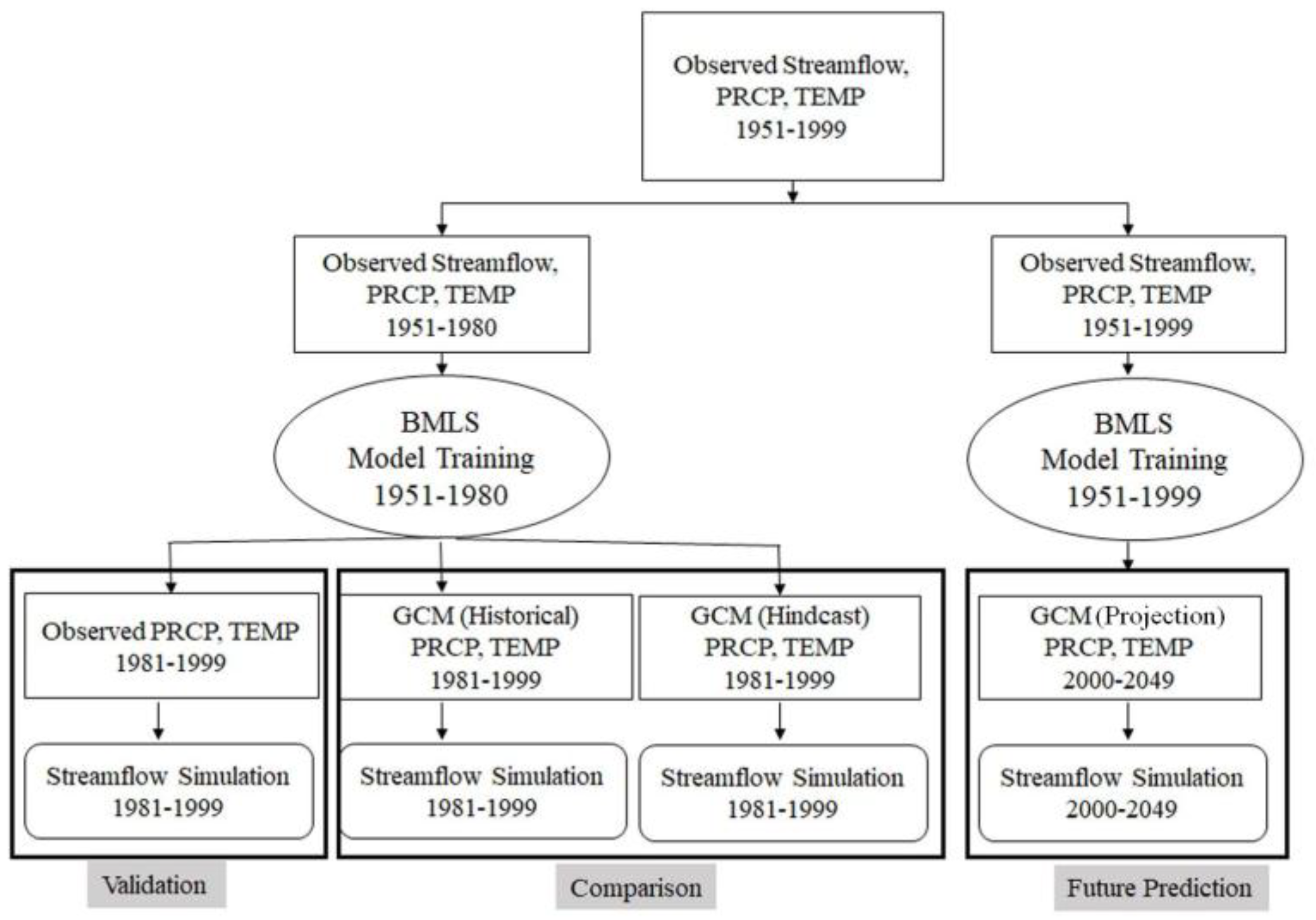
The observed dataset, consisting of observed streamflow, precipitation and temperature series, for the period 1951–1999 is divided into two parts. The first part contains two third of the data and is used for model training, while the rest of the dataset is used for model validation. The process is repeated three times as part of the three-fold cross-validation. Then, three GCMs’ outputs for the period 1981–1999 are applied to the model which is trained with observed climate predictors for the period 1951–1980. Streamflow simulations for 1981–1999, forced with GCM climate predictors, are used to compare hindcast and historical runs. Finally, the model is run with future projections of monthly
pr and
tas from 12 GCMs. For the future run, the model is recalibrated by considering monthly
pr and
tas data for the period 1951–1999 as predictors, while excluding streamflow from the predictor set (details are in
Section 4.3). Future changes in streamflow based on the past are evaluated. A schematic diagram of the carry-out plan is provided in
Figure 2.
Precipitation and temperature datasets from the GCMs have different spatial resolution than observed climate predictors. Hence, bilinear interpolation is applied on raw GCM outputs to bring the GCM resolution to the same as that observed, i.e., (1°
1°). Earlier studies [
30,
31,
32,
33] have reported that high amount of model bias existed in GCM simulations and argued the necessity of a performance-based model combination approaches. We apply a bivariate bias-correlation technique on GCM precipitation and GCM temperature. The technique, asynchronous canonical correlation analysis (ACCA), preserves the joint dependence between multiple variables while reducing bias in individual moments [
22]. For the current study, ACCA is applied to hindcast and historical outputs as leave-zero cross-validation basis. Modifications to the BMLS model requires a log-transformation on the streamflow. Therefore, back-transformation is applied to BMLS model outputs to bring the simulated streamflow back to the original space.
3.5. Test Statistics
The BMLS model is evaluated based on three-fold validation technique. Three-fold validation eliminates the possibility of overfitting, includes out-of-sample data, and exhibits the performance of the model under different climate conditions [
34]. The dataset containing the entire observed period (i.e., 1951–1999) is divided into three equal blocks. We have used two blocks for the model training while leaving the other block for model testing. Three conventional test statistics are used to evaluate model performance: reduction of error (RE), coefficient of efficiency (CE) and linear correlation coefficient (ρ). Cross-validation statistics values are shown later in
Section 4 as the average value of each statistic over the number of cross-validation folds, three for our study. The statistics are defined as follows:
where,
and
are the observed and model simulated streamflow at time step
t, whereas
and
is the long-term observed monthly streamflow respectively during the calibration and validation period.
RE and CE values range between +
to zero, whereas the linear correlation coefficient, also known as the Pearson correlation has a range between +1 to −1. A linear correlation value of zero suggests that there is no linear dependence between two variables of concern. From the definition of RE and CE, we interpret that if the test statistic value is lesser than one that indicates the model is better than climatology of the calibration and validation period, respectively for RE and CE. The use of climatology of the validation period makes CE more rigorous in comparison to RE. RE can be calculated for the calibration and validation period; however CE can only be calculated during the validation. The current study has modified the definition of RE and CE from the traditional definition [
34] which changes the range of these two cross-validation statistics. The change is made to ensure that the definition of RE or CE can be extended to compare performances between hindcast and historical runs (shown in
Section 4.2). Calculated RE or CE values can be subtracted from one to estimate the traditional values of RE or CE.
5. Discussion
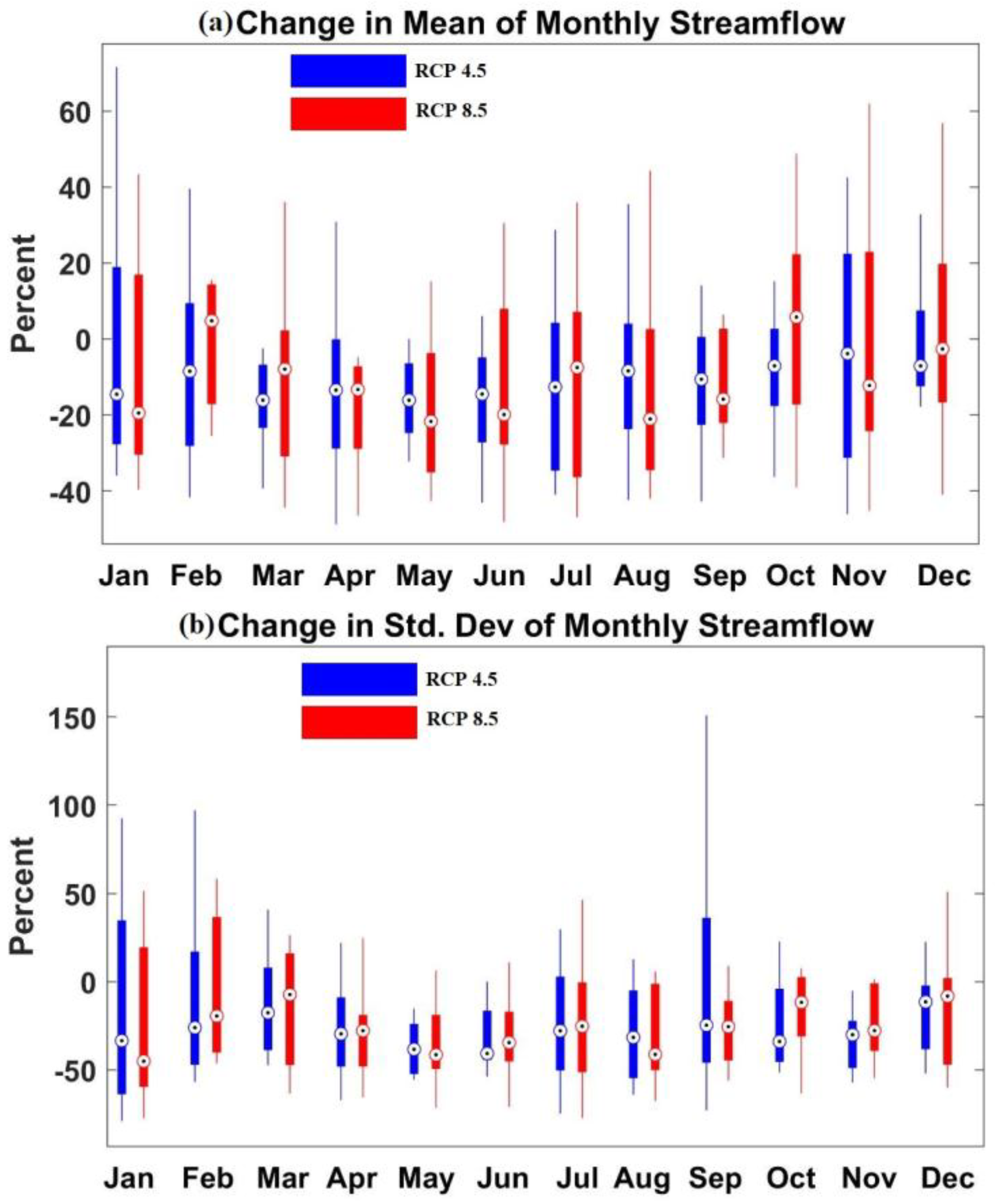
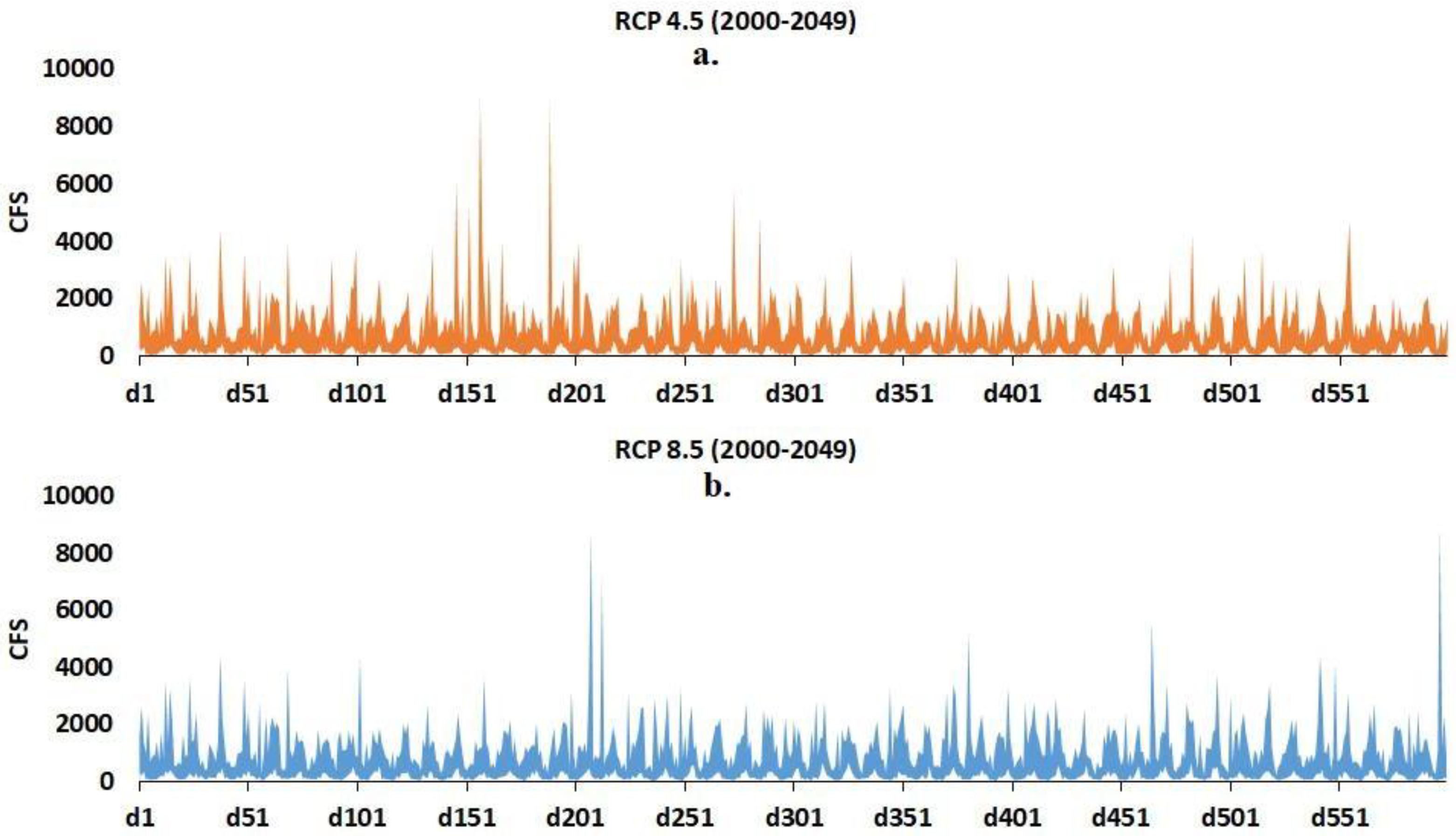
In this study, we modified and applied a novel statistical approach, BMLS, for monthly streamflow simulation. The BMLS model is applied for long-term streamflow simulation on an HCDN basin with lagged-streamflow, precipitation and temperature variables (for the future period, only precipitation and temperature) being the predictors. Firstly, we validated the BMLS model for the period 1951–1980 using observed precipitation and temperature and lagged observed streamflow inputs. Secondly, monthly streamflow is simulated by forcing GCM outputs from historical and hindcast experiments for the model validation period. Finally, future changes in streamflow are estimated based on future projections from twelve GCMs. The BMLS model is recalibrated with climate data (excluding lagged streamflow) from historical period (1951–1999) to project future changes streamflow for the period 2000–2049. Precipitation and temperature projections under two RCP scenarios (RCP 4.5 and RCP 8.5) from 12 GCMs are considered as predictors. Projected changes in the climate predictors have resulted from human-induced climate change. Hence, the changes in streamflow are also linked with the anthropogenic changes which are represented from RCP scenarios.
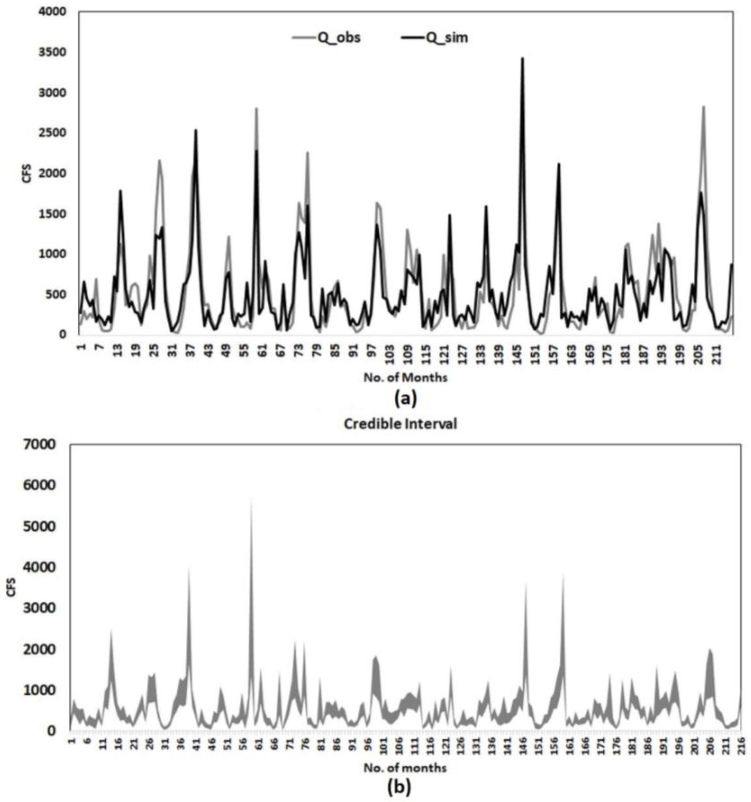
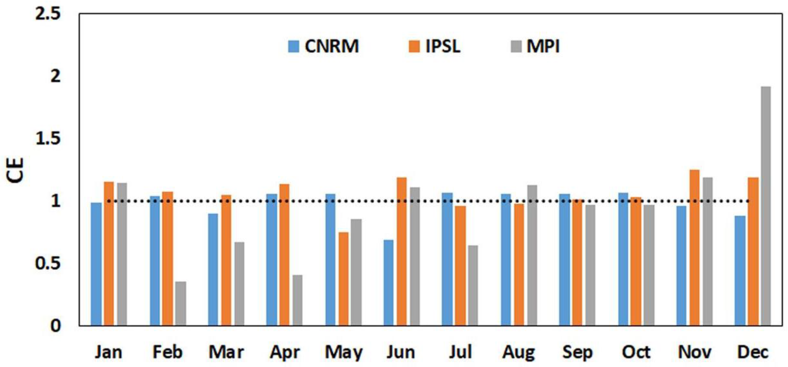
Validation results show that simulated streamflow exhibits significant information that is not presented in the climatology of the calibration or validation periods. The BMLS model exhibits RE and CE values lesser than one across all months during the validation period. Simulated and observed streamflow share a strong correlation during the validation period, except May, June, and October. Three-fold cross-validation, implemented to avoid the over-fitting of the model, exhibits a consistent performance of the BMLS model across the three validation sets. Results of streamflow simulations on the HCDN station, forced with GCM outputs, show that hindcast runs generally perform no better than the historical runs. Only one GCM hindcast, MPI, perform better than the GCM historical run on seven out of 12 months. The mean and the variability of streamflow on the HCDN basin is expected to decrease in future (2000–2049) under RCP 4.5 and 8.5. Percent change in future moments of monthly streamflow is estimated to be within 25% (40%) for the mean (standard deviation). The mean and variability of monthly streamflow on the gauging site are expected to decrease during 2000–2049. Changes in the streamflow could be associated with a future decrease in precipitation intensity, increase in the number of dry days across the south-east, and an increase in the average temperature. Swain and Hayhoe [
37] reported statistically significant increases in the mean spring standard precipitation index (SPI) over the northern part of the North American continent. Earlier studies have estimated a similar magnitude of change in river flow for the near, mid and long-term future. Campbell et al. [
38] predicted a change of −11% to +1% in the annual streamflow over a small watershed in the north-eastern United States. The magnitude and slope of the future change in streamflow depend substantially on the hydro-climate. For example, Chase et al. [
39] reported that two out of seven watersheds of eastern and central Montana would experience a decrease in the mean annual streamflow in the future, while the rest of the watersheds would experience an increase (decrease) in mean annual streamflow for the period 2021–2038 (2071–2088). Apart from the mean streamflow, the frequency of minor flooding over the near-term and mid-term future is also expected to increase under two RCPs along the coastal United States [
40].
Statistical models, in general, assume stationarity in projecting future changes, hence are not considered to be significantly reliable for climate change impact studies. Additionally, climate model uncertainty and scenario uncertainty result in a significant prediction uncertainty in the future streamflow. Despite the shortcomings of statistical techniques, our study confirms the applicability of the BMLS model for long-term streamflow simulation. Model calibration and validation results indicate that the model could be useful when the watershed information is limited, and a large number of climate predictors are present. Consistent performance of the model leads us to perform additional experiments with CMIP5′s historical and hindcast runs. We suggest that no further benefit can be achieved in streamflow simulation by replacing historical runs with decadal predictions. Nevertheless, hindcast projections are useful for streamflow simulations of 30 years or less. For a simulation of more than 30 years, the study suggests using long-term climate projections to estimate the future changes. A decrease in the monthly streamflow would result in additional stress on water resources planning. A future study should examine the impact of the reduction in the mean of monthly streamflow on downstream reservoirs, and the soft and hard-path strategies to replenish the deficit.
The BMLS model allows predictors with a spatial resolution different from that of the predictand. Unlike process-based models like SWAT or PIHM, the BMLS model does not necessarily require pre-processing of climate model outputs. Such pre-processing may include predictor selections, bias-correction and spatial downscaling, etc. Earlier studies have reported that the pre-processing of climate predictors can potentially include significant uncertainty in the streamflow simulation [
26,
41,
42]. However, the current study has applied a multivariate bias-correction technique, ACCA, to remove model bias in climate predictors while preserving the interdependence between precipitation and temperature. A future study to evaluate the difference between the hindcast and historical runs should include multiple stream-gauge sites to provide a comprehensive understanding of the problem. The current study does not estimate the statistical significance of the CE values estimated using hindcast and historical runs (
Section 4.2). A non-parametric bootstrap approach can be applied to test the statistical significance of the CE values. The null hypothesis would state that CE value is equal to one, i.e., RMSE exhibited by hindcast, and historical runs are the same. Readers are encouraged to read Goddard et al. [
23] for details regarding the non-parametric bootstrap approach in the context of a decadal experiment’s verification. The similar performance of historical and hindcast runs as climate predictors are attributed to the efficiency of the ACCA technique because predictor uncertainty is considered as one of the dominant sources of the uncertainty in simulated streamflow [
26]. In conclusion, the quality of GCM outputs eventually does not vary between SST initialized and non-initialized climate model runs.
Future improvement of the current model can be achieved by considering informative prior selection, incorporating predictor selection algorithms and adopting a sensitivity analysis to achieve a thorough understanding of the model parameters. Although the current study considers a single station, selection of multiple HCDN stations across various climate regions of the United States would provide a comprehensive understanding of the reversibility of the BMLS model on multiple basins. Including climate indices and teleconnection, such as SST, ENSO, and PDO, is expected to ensure an improved simulation of streamflow. Predictor uncertainty can be reduced by considering observed climate variables with finer resolution. An increase in the number of GCMs for future assessment is expected to reduce the model uncertainty and improve accuracy [
43,
44,
45,
46,
47]. Finally, the study confirms the applicability of a novel Bayesian approach for streamflow simulation and concludes that the approach can be useful in assessing the impacts of climate change on water resources.


