Labeling Water Transport Efficiencies

Abstract

Pressurized Water Transport Systems (PWTSs) are responsible for a large percentage of the electricity consumption around the world, and current trends suggest that this proportion will continue to increase in the future. Controlling PWTS is therefore fundamental, including improving efficiency when necessary or compulsory. To achieve this, metrics to objectively assess the efficiency of the different losses and of the whole system are needed. These metrics, based on economic criteria, will be stricter if environmental costs are added to current water and energy costs. To assess different improvement strategies, some relative metrics, applied to both operational and structural losses, are considered. At the end, taking into account their relevance, these metrics are combined in a global energy score (IS), this being the main contribution of this paper. Finally, to focus on the concepts and methodology, a simple case study is presented.

1. Introduction

Most of the world’s fluid transport (measured in t × km) is via pipelines. The significant weight of fluids is a contributing factor especially for water and oil, as are the growing demand for these fluids. In Spain, for example, piped water transport accounts for 66.6% of the total, distantly followed by highway transport (28.3%) [1]. This results in an overwhelming percentage due to an obvious fact: only fluids can be transported by pipe. Moreover, nothing suggests that this situation will decrease in the future. Therefore, more efficient piped fluid transport is required. Specific data also confirm this claim.

In fact, 6% of the total consumed electrical energy in California is due to water transport [2], whereas in Spain, irrigation water alone accounts for 3% of the total [3]. Logically, this energy consumption is not only due to water transport inefficiencies. Gravitational energy due to elevation changes and working pressure are also energy requirements for different usages.

To optimize Pressurized Water Transport Systems (PWTSs), work in two directions must be complete. Firstly, fostering improvement strategies from a technical point of view, such as energy efficiency diagnoses and audits on these systems, must be undertaken, as well as raising awareness among managers, which includes informing and encouraging them. This requires metrics that indicate the level of losses in managed systems are reasonable, in accordance with the current state of the art technologies and standards. This should be globally applicable and easily understood, even for people without specific technical training. This need has already been underlined [4] but our current proposal provides further understanding. The main contribution of this paper is providing a metric that summarizes the global system energy performance, gathering together and weighting all systems’ losses, including pumping, leakage, and friction losses. Decoupled analysis of each type of loss, with their corresponding metrics, can be widely found in the literature: pumping station losses [5,6], leakage losses [7,8], pumping and leakage losses simultaneously [9], friction losses [10,11], and pumping and layout (structural) losses [12]. Conversely, pipe-level metrics are available [13], although a global metric based on a well-funded protocol is missing, which was the main objective of this paper.

Global analysis is the only method that can be used to optimize efficiency. Pressurized water transport entails different types of inefficiencies, which have only been addressed separately to date. Efficiency of pumping systems in PWTSs is a clear example of the need to conduct extensive analyses. The European Union has fostered a directive imposing minimum pumping performance [14]. Moreover, pump manufacturers have warned that regardless of pump efficiency, if the right pump is not fitted, performance of the assembly can still be very poor. Consequently, the scope has been extended from only considering pump performance to defining an Energy Efficiency Index (EEI), which considers the performance of the pump and the load curve assembly as a whole, within the new Extended Product Approach concept (EPA) [6]. To maximize efficiency, the system curve must be previously optimized.

Consequently, in a global process, the first step is to analyze the system as a whole, then optimize the load system curve, and finally work downward to select the right elements. For example, if the layout is not optimum [15], neither is the system curve nor will the system as a whole be efficient, even if the EEI and the pumping equipment are optimized. It is, therefore, necessary to perform global analyses.

The overall energy efficiency requires jointly analyzing the three parts of the system while simultaneously studying their interdependencies. These parts include the following: (1) Energy sources. Two different types can be considered: Tanks, which are rigid energy sources (RES) and pumping stations, which are variable energy sources (VES). The energy injected into the system by RES is constant, providing variations in the water tank levels are not taken into account. Energy supplied by VES can meet the system’s requirements by changing the pump’s rotational speed [15]. (2) Piping system and other necessary elements for transporting water, i.e., from a single diameter pipeline to a complex system, with numerous nodes and loops. (3) Points of use, where transported water is delivered. The simplest case would be a tank. In an urban water network, points of use refer to users’ installations, whereas in irrigation networks, it refers to final pipes inside the plots supplying sprinklers or drip-irrigation devices.

Once these three parts have been integrated in a PWTS, they create an entire system with a specific layout, largely dependent on the topography that notably affects its energy performance. Achieving the highest efficiency is only possible from a global analysis approach, covering these three parts and without ignoring the framework where it is located.

Previous studies [16,17,18] described how to perform this global analysis, whereas this article proposes partial and global metrics. The remainder of the paper is organized as follows. In Section 2, system assessment is discussed [16]. The difference between single pipelines and networks and between ideal and real systems are considered and results discussed. Notably, the diagnoses assess the overall energy efficiency, but without providing information on where and how much energy is lost in each phase of the PWTS. Next, the system audit is analyzed [17]. Water and energy audits are required to identify which part of the total energy losses corresponds to each inefficiency. However, metrics are needed to assess the significance of each kind of loss, which is the objective of the next stage. Then the relevance of each kind of loss is evaluated. It is crucial to know whether these losses are excessive, reasonable, or if their current level will be difficult to improve. The proposed reference values are based on economic criteria. Finally, an equation to integrate these partial efficiencies into a single value is proposed. This score that can be used to label the system. Afterward, a simple case study to clarify the methodology is presented. This methodology can be extended to real systems following the concept herein developed. In fact, from the basic example of this paper, the energy audit of a real case (Bangkok water network) has been recently performed [19].

2. Energy Assessment of PWTSs

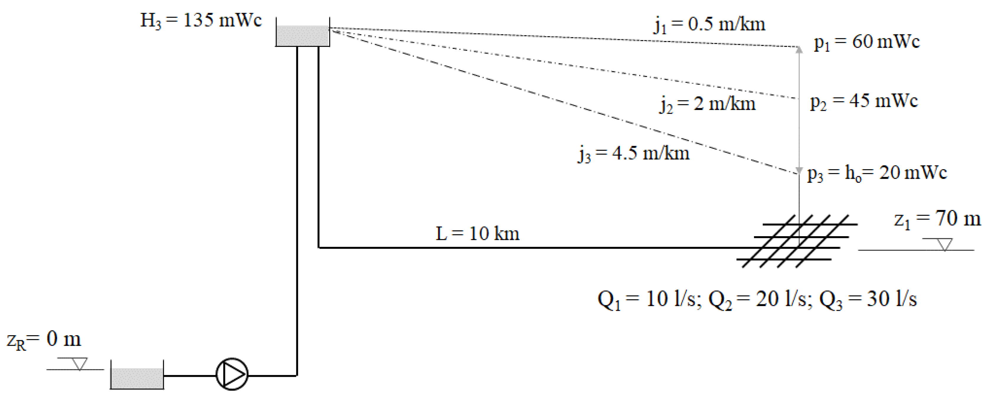
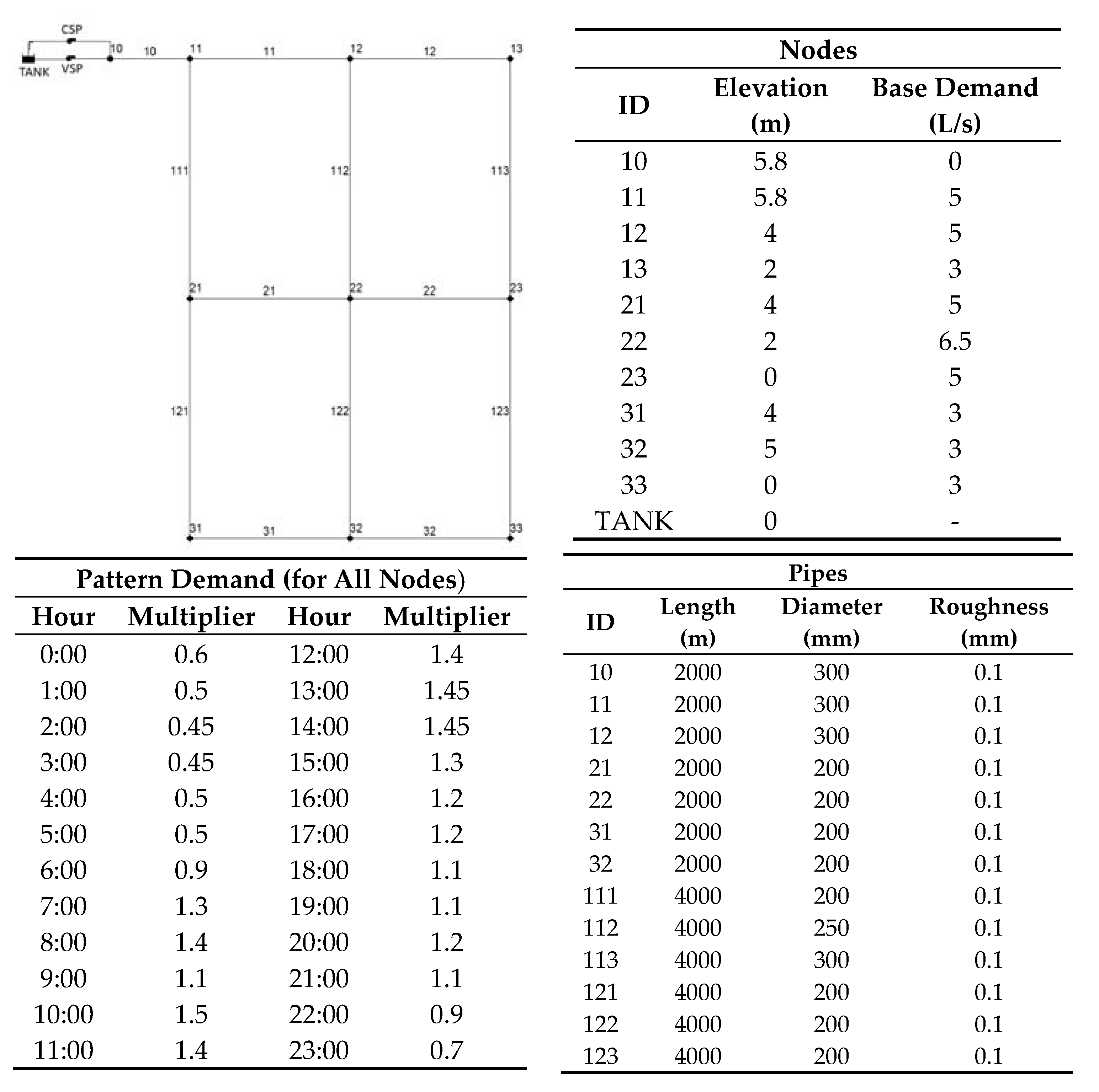
Assuming no operational losses (ideal case), the following data are required to diagnose a system: (1) elevation of the water source, (2) elevation of the demand points z_j with their corresponding consumed volumes v_j, and (3) pressure at the delivery points. In urban networks, pressure is set by the standards, whereas in irrigation networks, it depends on the requirements of drippers or sprinklers, which is zero when a tank is filled.

The simplest case, also fairly common, is pumping water from an aquifer to a tank with a simple pipeline from source to delivery point. Assuming H = 100 m of elevation head, a flow Q = 0.1 m³/s, which is 8640 m³/day, and no pressure requirements at the delivery point (i.e., a tank), the daily consumed energy is:

$$E=\gamma QH=2354.4 \mathrm{kWh}/\mathrm{day}$$

(1)

Energy intensity I is measured in kWh/m³, and the relation between the energy consumed and the pumped volume is 0.2725 kWh/m³. This is the energy required to pump one cubic meter an elevation of 100 m. This is an ideal value because transport inefficiencies (friction, leaks, or pumping losses) have not been included.

The indicator generally used is 0.4 kWh/m³ per 100 m elevation. It is assumed that friction losses are 10% of the elevation head (a rather exaggerated figure, only justifiable with long distance water transfer), a pumping efficiency of 75% (a reasonable value), and a non-leaky pipeline. Therefore:

$$I=0.2725 \mathrm{kWh}/{\mathrm{m}}^3 \times 1.1 \times \frac{1}{0.75}=0.4\mathrm{kWh}/{\mathrm{m}}^3$$

(2)

In a previous paper [16], this concept was generalized for water networks. Although from a conceptual point of view, the single pipeline network approach is identical, there are three differences to underline. (1) The existence of consumption points at different heights and with different demands, which introduces two new related concepts: topographic energy and structural losses. These concepts are not logical in pipelines. (2) Network water leaks in practice are unavoidable. This introduces a third type of loss in addition to those mentioned for the simple pipeline. (3) Water supplied at demand points must be delivered at a required pressure (p_o/γ = h_o).

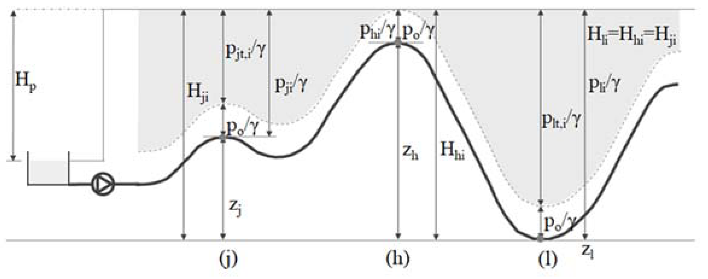
As such, how to assess the performance of an ideal network is summarized. Further details are provided in a previous study [16]. Figure 1 shows the profile of one pipe of the network that includes intermediate water consumption points. The supplied energy is conditioned by the highest node (z_h) and by the minimum pressure to deliver to users, p_o/γ = h_o. The heights must refer to the lowest non-zero flow node (z_l). Under these conditions, the efficiency (η_ai) is the relation between the minimum energy required to supply to consumers E_uo and the energy injected into the system E_si:

$${\eta }_{ai}=\frac{E_{uo}}{E_{si}}$$

(3)

where

$$E_{uo}=\gamma {{\displaystyle \sum }}^{\text{}}{v}_j\left[\left(z_j-z_l\right)+\frac{p_0}{\gamma }\right]$$

(4)

and

$$E_{si}=\gamma V{H}_{hi}=\gamma {{\displaystyle \sum }}^{\text{}}{v}_j\left[\left(z_j-z_l\right)+\frac{p_{ji}}{\gamma }\right]=\gamma {{\displaystyle \sum }}^{\text{}}{v}_j\left[\left(z_j-z_l\right)+\frac{p_0}{\gamma }+\left(z_h-z_j\right)\right]$$

(5)

where V is the total volume to supply in the given period and, if there are no leaks (ideal system), is the sum of all nodal demands, ($V={{\displaystyle \sum }}^{\text{}}{v}_j$), and $H_{hi}$ is the piezometric height of the highest node.

The ideal topographic energy E_ti can be defined as the excess of energy delivered to each node, as shown in Figure 1, thus obtaining:

$$E_{ti}=\gamma {{\displaystyle \sum }}^{\text{}}{v}_j\frac{p_{jt,i}}{\gamma }=\gamma {{\displaystyle \sum }}^{\text{}}{v}_j\left(z_h-z_j\right)$$

(6)

Which shows a balance: the total energy injected into an ideal system is the sum of the strictly necessary energy, plus an energy surplus, referred as topographic energy.

$$E_{si}=E_{uo}+E_{ti}$$

(7)

Notably, the concept of topographic energy is tied to two facts. First and most important, topographic energy is the link to the land topography, hence its name. With delivery nodes at different heights, this energy will always exist. Since sufficient energy must be guaranteed for the least favorable node, an excess of energy is supplied to the lower nodes. Unlike the previous operational losses, such as leaks or friction, named structural losses. The second factor is linked to RES because, when located higher than necessary, topographic energy in flat areas is generated (Figure 2).

By combining Equations (3) and (7), the efficiency of an ideal water distribution network is obtained:

$${\eta }_{ai}=\frac{E_{uo}}{E_{si}}=1-\frac{E_{ti}}{E_{si}}=1-{\theta }_{ti}$$

(8)

where θ_ti is the contribution of the structural losses in decreasing the system efficiency. The structural losses can only be reduced through layout modifications (structural actions). Strictly speaking they are not losses as such because energy is not dissipated but, they are responsible for additional energy being supplied to the system.

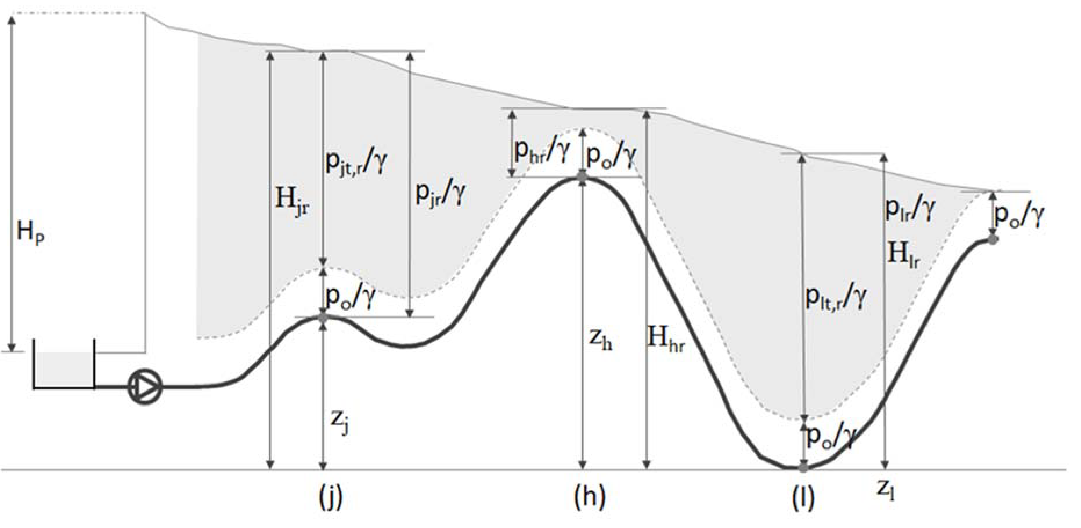
In real systems, the energy injected into the system is, to a greater or lesser extent, higher than E_si. Figure 3 shows a real system [16] where even more pressure than the minimum required is delivered to the least favorable point. In an energy balance of a real system, the following differences apply:

(1)

The energy E_uo is identical in both cases because it only depends on the user demands and the service requirements. This is not the case for the total supplied energy in a real system E_sr, which must include losses.

(2)

The operational losses, modifying the piezometric height lines, are energy dissipated through friction in pipes and valves (E_rf), energy embedded in leaks (E_rl), and pumping station inefficiencies (E_rp).

By merging all these real operational losses in E_ro, can be stated:

$$E_{ro}=E_{rp}+E_{rf}+E_{rl}$$

(9)

The real topographic energy E_tr (Figure 3, shaded area) is different to the ideal E_ti. E_tr is now linked to the new real piezometric height which, with losses, is no longer horizontal. Finally, another type of energy loss exists, the real avoidable losses E_ra, which are relatively common. These include excesses of energy delivered at the least favorable node (Figure 3) and depressurization in domestic tanks.

In short, analysis of ideal systems sets the maximum values for system efficiencies. Real systems share the energy efficiency numerator (E_uo) with ideal systems, but the denominator, E_sr, is substantially different, as shown in Equation (10). That supplied energy can proceed from a RES, natural source E_N, or from a VES also called shaft energy E_P, [17]. Therefore:

$$E_{sr}=E_{uo}+E_{tr}+E_{rf}+E_{rl}+E_{rp}+E_{ra}=E_{uo}+E_{tr}+E_{ro}+E_{ra}=E_N+E_P$$

(10)

Ultimately, the real efficiency η_ar results from:

$${\eta }_{ar}=\frac{E_{uo}}{E_{sr}}=1-\frac{E_{ro}}{E_{sr}}-\frac{E_{tr}}{E_{sr}}-\frac{E_{ra}}{E_{sr}}=1-\frac{E_{ro}}{E_{sr}}-{\theta }_{tr}-\frac{E_{ra}}{E_{sr}}$$

(11)

Shaft energy E_P is determined from the electricity bill, whereas natural energy E_N can be directly estimated [17], so therefore η_ar can be calculated. η_a is the ideal performance less the contributions of the operational losses E_ro, the structural losses E_tr represented by θ_tr (topographic energy indicator), and, if any, the avoidable losses E_ra.

3. Operational and Structural Losses Metrics: Final Labeling

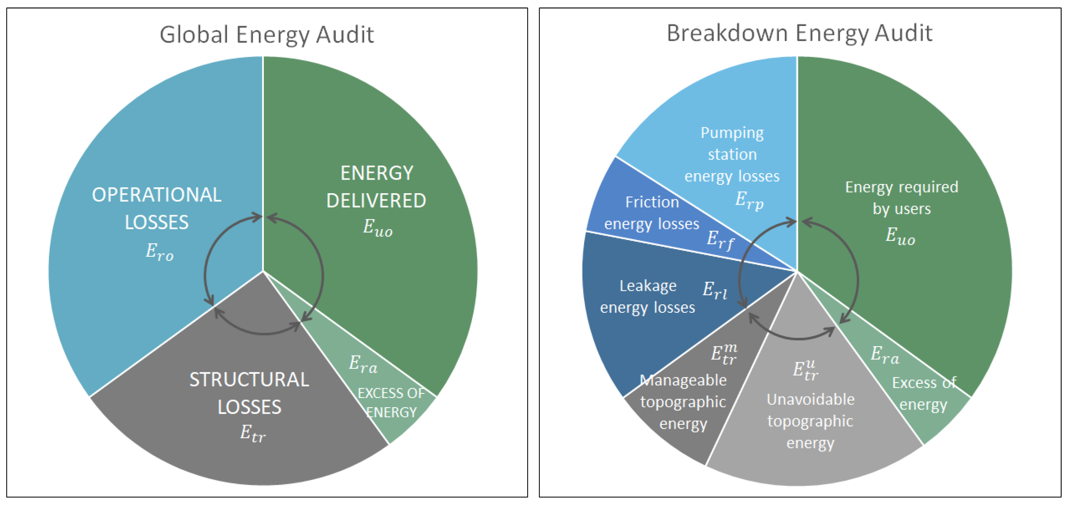
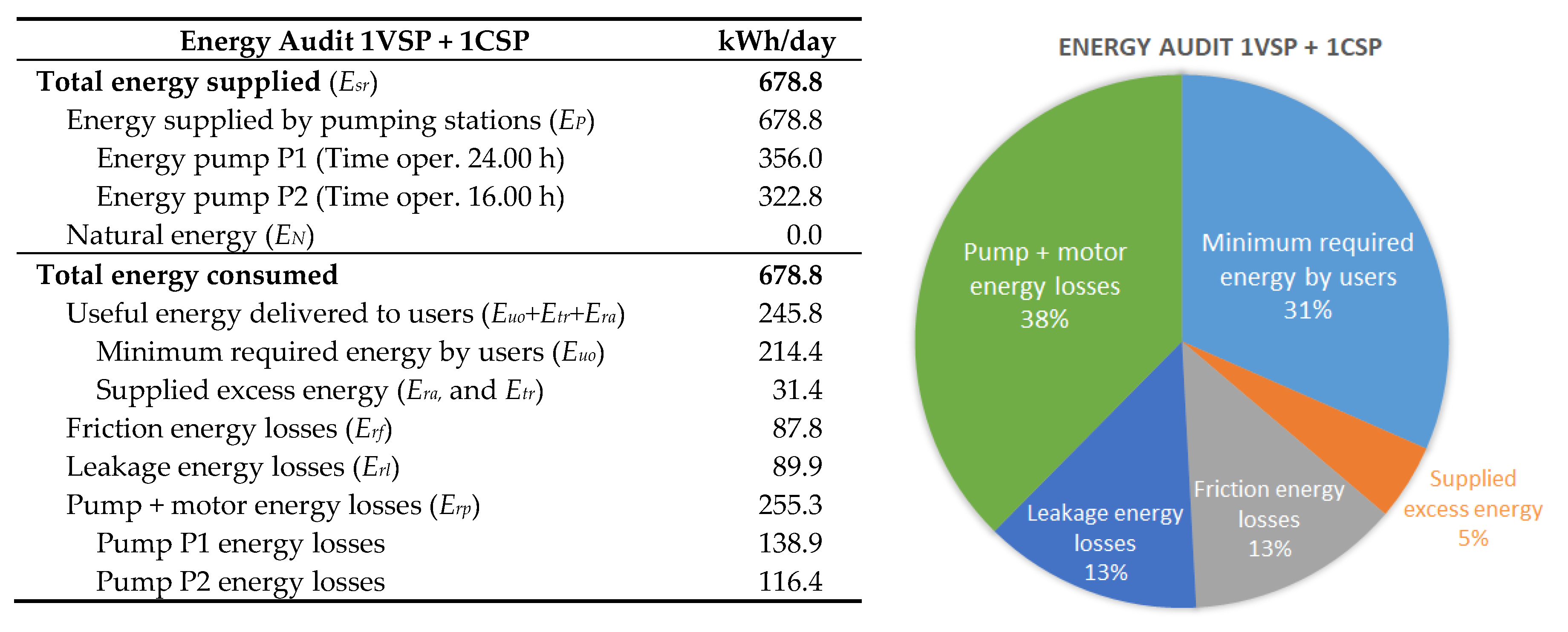
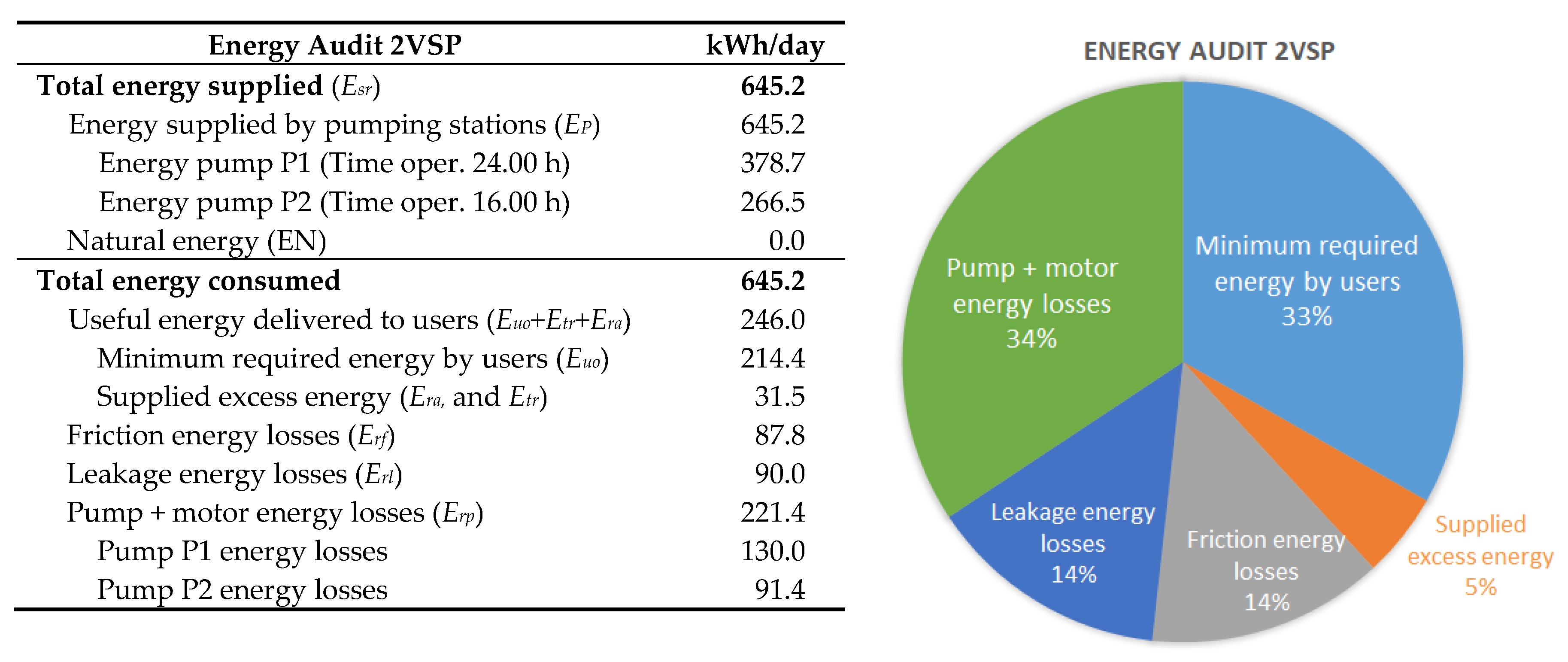
After the assessment, the system is audited, firstly from a water point of view [20] and then in terms of energy [17]. Figure 4 summarizes the results for a network without domestic tanks, and therefore the only avoidable energy E_ra is the excess of pressure. The left of the figure shows the general summary according to Equation (9), and the right shows the losses that have been broken down according to Equation (10). The topographic energy has also been separated. Part of this energy can be managed by recovering it with pumps as turbines (PATs) or dissipating through pressure reducing valves (PRVs), resulting in the manageable topographic energy concept, $E_{tr}^m$. The complimentary term is the unavoidable topographic energy $(E_{tr}^u$), which will inevitably continue to be part of the system’s energy balance unless the layout is changed [15].

The system as a whole is coupled and therefore operational losses are interdependent. Reducing leaks diminishes friction and simultaneously modifies the operating point of the pumps. However, as the losses are identified and the equations to assess them are decoupled, the losses can be calculated separately [17]. Operational losses are produced in two of the three parts of the system. Losses occur if the energy source is a VES. The transformation of electrical energy in hydraulic energy involves losses that do not exist if the energy comes from a RES, as hydraulic energy is supplied directly without any transformation process. The other two operational losses, friction and leaks, are in the second part of the system in the network pipes, whereas structural losses are at the consumption nodes, corresponding to the third system stage.

Finally, the two kinds of avoidable losses must be considered. The first one, depressurization in domestic water tanks (if any), occurs between the second and third stages. Although there is no loss of water, this inefficiency is similar to a leak from an energy point of view, and therefore can be considered an operational loss. The second avoidable loss is delivering more energy than necessary at the least favorable point and consequently to the entire system. Removing these losses entails reviewing how the energy source works. If the energy source is a RES, the loss is unavoidable and can be classed as an additional structural loss. If the source is a VES, the loss can be minimized using variable speed pumps and should be considered an operational loss.

Once the audit has been performed, the next stage is to identify reference levels, i.e., metrics that permit assessing the relevance of each kind of loss. This allows identifying if losses are excessive, reasonable, or if they are low enough that reducing them further is not practical. This analysis is crucial to determine the priority of actions considered to improve the energy efficiency and, furthermore, to label the global efficiency of the system [21]. The case study will show that a simple quantitative analysis without reference levels can lead to some misleading conclusions.

3.1. Energy Losses Reference Levels

The suggested reference levels are provided for operational losses and structural losses.

3.1.1. Operational Losses, E_ro

E_rl is the leakage energy losses. Two reference levels, the Economic Level of Leakage (ELL) [22] and alternatively the Infrastructure Leakage Index (ILI) [23], can be used.

E_rf represents the friction losses. A previous study provided a similar metric to ELL, called the Economic Level of Friction (ELF) [10], which can be more or less stringent by adding environmental taxes to the energy costs.

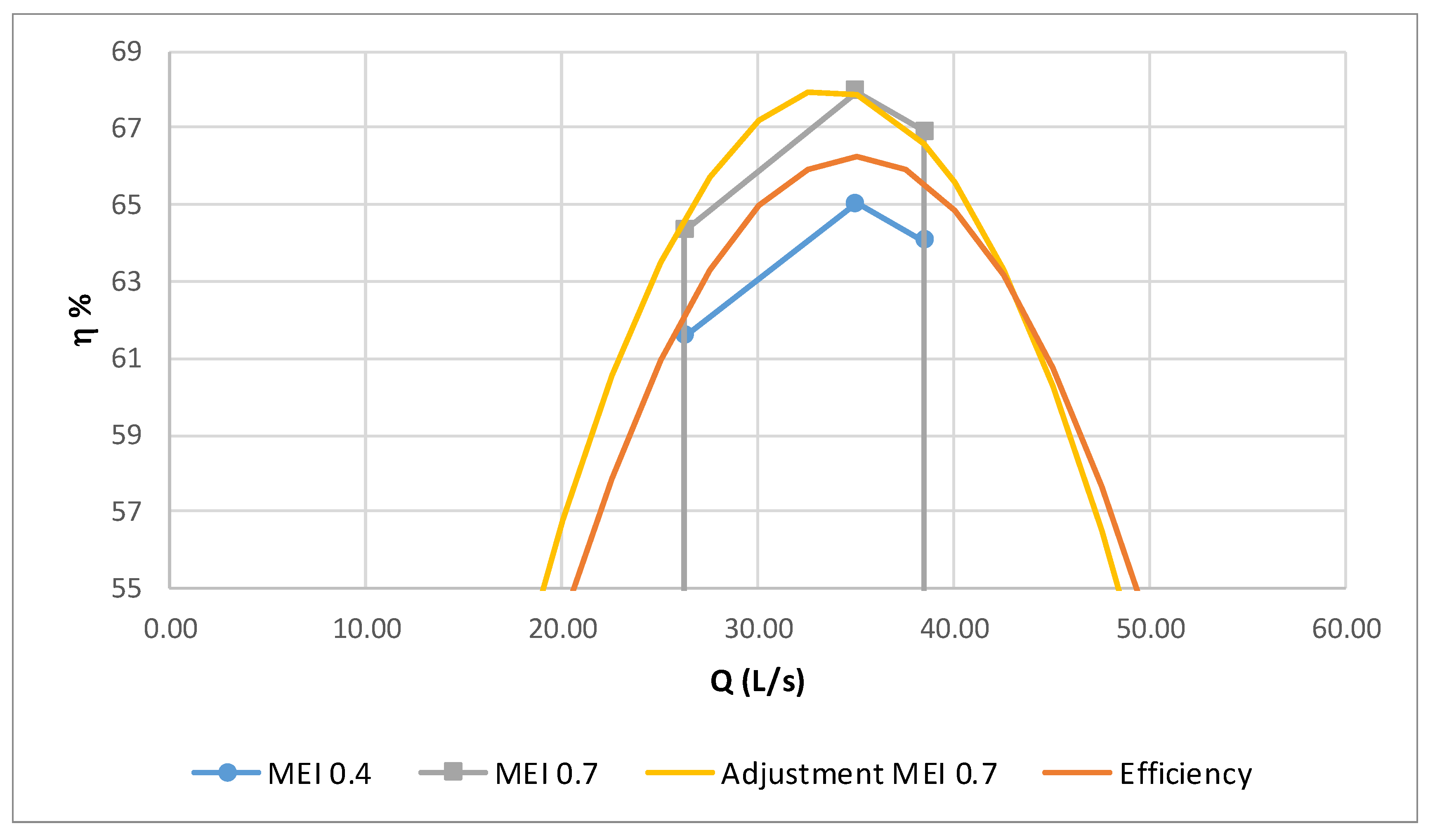
E_rp represents the pumping station losses (wire to water inefficiencies), referred to the pump only, the Minimum Efficiency Index (MEI). This concept has been defined by the European Commission [14], a criterion extended to the EEI [6], when pumps and motor driven efficiency are considered as a part of the PWTS, such as when coupled to the system load profile. The minimum MEI considered [14] is 0.4 and was adopted for PWTS working for a low number of hours per year (h_w), which is considered to be less than 500 h/year, such as in fire-fighting systems. For higher h_w, a MEI of 0.7 will be adopted. In this new context, with compulsory minimum efficiencies, a pump life cycle cost analysis does not make sense [24]. Although the system’s manager can address some losses (e.g., leaks and friction), pump losses cannot be easily changed. They depend on the state of the art and on the right pump selection.

3.1.2. Structural Losses, E_tr

Structural losses E_tr weighted by θ_tr, the topographic energy indicator, can be split into manageable topographic energy and unavoidable topographic energy. Manageable topographic energy can be partially recovered with PATs or partially removed with PRVs [15]. Being very much dependent on the PWTS load conditions, a reference level does not make sense. Its relevance is indicated by the manageable topographic energy indicator, ${\theta }_{tr}^m=\frac{E_{tr}^m}{E_{tr}}$.

$E_{tr}^u$ is unavoidable topographic energy that depends on the network’s topography. It can only be reduced by modifying the system’s layout [15]. Being independent of the management quality, a reference level does not make sense. Its relevance is demonstrated by the unavoidable topographic energy indicator, ${\theta }_{tr}^u=\frac{E_{tr}^u}{E_{tr}}$ and ${\theta }_{tr}={\theta }_{tr}^m+{\theta }_{tr}^u$.

Lastly, avoidable losses $E_{ra}$ do not require reference values. They can be, and therefore should be, zero.

3.2. Global Energy Losses Score

The next step was to calculate an energy score for the entire PWTS. The reference levels for losses provide specific values and are of a local nature since they are linked to water and energy costs and can be more or less sensitive to environmental targets by including taxes in their costs.

Table 1. Reference levels for operational losses.

Energy Loss Type	Reference Level
Leakage	ELL is used as economic leakage losses reference level, El,e.
Friction	ELF is used as economic friction losses reference level, Ef,e.
Pump	EEI is used as economic pumping losses reference level Ep,e. (MEI = 0.4 for low hw values and MEI = 0.7 for high hw values).

summarizes these economic and environmental criteria.

Once the criteria have been established, these levels ($E_{l,e}$, $E_{f,e}$, and $E_{p,e}$) must be calculated for the analyzed system. From the energy audit, leaks and friction energy real losses, $E_{rl}$ and $E_{rf},$are known, respectively (Figure 4, right). From the ELL, the economic level of leaks concept,$Q_{l,o}$ is determined, whereas from the ELF procedure, the optimum average unitary head loss, $J_o$, is calculated. With the present level of leaks $Q_l$ and actual average friction J_a, the reference values $E_{l,e}$ and $E_{f,e}$ can be finally determined, respectively, according to:

$$E_{l,e}=\frac{Q_{l,o}}{Q_l}{E}_{rl} E_{f,e}=\frac{J_o}{J_a}{E}_{rf}$$

(12)

However, E_l,e cannot be directly determined because it depends on the adopted MEI and on the system’s characteristic load. It must be calculated from the mathematical model of the network. Equation (13) summarizes this result:

$$E_{p,e}=f\left(\mathrm{MEI}; \mathrm{PWTS} \mathrm{pumping} \mathrm{characteristic} \mathrm{load}\right)$$

(13)

The global economic energy loss reference $E_{o,e}$ is determined with:

$$E_{o,e}=E_{l,e}+E_{f,e}+E_{p,e}$$

(14)

whereas the score for the proposed global energy index I_S is:

$$I_S=\frac{E_{rl}}{E_{l,e}}\frac{E_{l,e}}{E_{o,e}}+\frac{E_{rf}}{E_{f,e}}\frac{E_{f,e}}{E_{o,e}}+\frac{E_{rp}}{E_{p,e}}\frac{E_{p,e}}{E_{o,e}}= \frac{E_{rl}}{E_{l,e}}{\gamma }_l+\frac{E_{rf}}{E_{f,e}}{\gamma }_f+\frac{E_{rp}}{E_{p,e}}{\gamma }_p$$

(15)

where γ_l, γ_f, and γ_p are the weighting factor of leakage, friction, and pump losses, respectively. The optimum value of I_S is one. The higher the value of I_S, the worse the score.

This global energy score I_S represents the weighted operational losses efficiency. Without structural losses metrics, three context performance indicators can be used to provide an idea of its relevance. Two of these indicators,${\theta }_{tr}$ and ${\theta }_{tr}^m$, or their complementary value ${\theta }_{tr}^u$, have been previously defined. The third indicator C₁ clarifies the origin of the energy (natural or shaft) and is given by C₁ = E_N/E_sr [17]. Ultimately, ${\theta }_{tr}$, ${\theta }_{tr}^m,$ and C₁ provide clear information about the relevance of the structural losses and the potential for their reduction. To summarize, the operational losses global score in Equation (15) indicates the efficiency of a PWTS, and could be the basis for a final label, whereas the three structural parameters provide clear information about the framework in which the system operates.

4. Case Study

The network (Figure 5) was adapted from a case study used in a previous paper [17]. It is a simple system to allow focusing on the methodology, so showing the relevance of the reference metrics for each kind of loss is adequate. The quantitative audit result can be misleading and result in bad decision-making. The example corresponds to an urban network.

4.1. Basic Data

In terms of layout, the network length (L_t) is 40 km, the number of service connections (N_c) is 4000, and the total length of service connections (L_a) is 40 km. In terms of volume and leaks, the supplied volume (V) is 4684.6 m³/day, consumed volume (V_U) is 3423.4 m³/day, the leakage volume (V_L) is 1261.1 m³/day, the Technical Indicator for Real Losses (TIRL) calculated by V_L/N_c is 315 L/connection day, and the marginal cost of water is 0.25 €/m³. The Active Leakage Control Curve (ALCC) is C (€) = $2 \times {10}^8 \times Q_l^{-0.715}$, denoted by Q_l in m³/year. In terms of pressure, the minimum pressure according to standards calculated by p_o/γ is 20 mWc and average pressure ($\overline{p}$) is 23.6 mWc. For the working pumps, H_p(m) is 46 – 0.007292 Q² (L/s), η_p is 0.03796 Q – 0.00054 Q² (L/s), the electric motor efficiency IE3, η_m is 0.921 (power (P) = 15 kW; speed (N) = 1450 rpm) and working hours/year (h_w) is 8760. Finally, the energy costs for each daily period (€/kWh) are 0.083, 0.15, and 0.22, and the energy supplied is the shaft energy when tank elevation is the lowest (C₁) is 0.

4.2. Energy Audit Results

A water audit was previously performed; Figure 6 condenses the results of the energy audit that was completed as the system is operating. The first pump works at a constant speed (CSP), whereas the second pump is a variable speed pump (VSP). The minimum required energy accounts for 31% of the total energy supplied and consequently the real overall efficiency is ${\eta }_{ar}$= 0.31. Operational losses, 64%, account for a significant part of the energy balance and the objective was to identify the margin for improvement of each type of loss.

Before calculating the reference values for the losses, the working conditions of the two pumps were analyzed. In the initial pumping system (one CSP and one VSP), both pumps frequently operated outside the recommended working points. These extreme points are the partial load flow rate Q_PL, 75% of the Best Efficient Point (BEP) flow Q_BEP, and the overload flow rate Q_OL, equal to 110% of the Q_BEP. The reference flow is Q_BEP [14].

To enable further adjustment, a simulation with two VSP was performed. The results, depicted in Figure 7, show an improvement of around 5% because most of the working points were within the recommended range. However, as the percentages refer to the total energy demand, which is different in each case, the dissipated pumping energy is examined. In the first case 255 kWh/day was required, and 221 kWh/day was required in the second cased, because with two VSP, the working points were closer to the BEP. In summary, for one CSP and one VSP, the working points are outside the recommended range for 15 h, with a minimum of 36.6% and a maximum of 140.4% over Q_BEP, whereas with two VSP, the system only operates outside the range for three hours, with a minimum of 66.6% and a maximum of 118.4% over Q_BEP.

This is a remarkable but inconclusive finding because the efficiency of the variable speed driver, which would further hinder the two VSP solution, has not been included. Whichever the case, since this has a minimal impact on the global energy index I_S, the system baseline is considered to be having one CSP and one VSP, as depicted in Figure 6. The system’s average pressure over time and space is 23.6 m; this value is necessary for later calculations.

4.2.1. Pumping Losses Reference Levels

The results of the system operation (one CSP and one VSP in Figure 6) were compared to the curves whose minimum performance value was previously reported [14]. Basically, the equation that sets the minimum pump efficiency (based on Q_BEP, in m³/h) and the specific speed n_S (in min^–1) is:

$${\eta }_{BEP}=-11.48(\ln {\left(n_s)\right)}^2-0.85(\ln {\left(Q_{BEP})\right)}^2-0.38\ln \left(n_s\right)\ln \left(Q_{BEP}\right)+88.59\ln \left(n_s\right)+13.46\ln \left(Q_{BEP}\right)-C$$

(16)

In our case, Q_BEP = 35 L/s = 126 m³/h, N = 1450 rpm, and H_BEP = 37.74 m, resulting in n_S = 17.82 min^–1. From these values, η_BEP is calculated as:

$${\eta }_{BEP}=199.84-C$$

(17)

where the constant C depends on the MEI and the type of pump selected. In this case,

Table 2. Minimum required pump performances for ESOB 1450 pumps [16].

Value	MEI = 0.7	MEI = 0.4
C	124.85	128.07
Efficiency QPL	71.02	67.97
Efficiency QBEP	74.99	71.77
Efficiency QOL	73.87	70.70

summarizes the complementary values to determine the minimum required performance [16]. The values were not as high as expected (Figure 8) because all the performed analyses include the efficiency of the alternating current (AC) electric motors as well. The actual pumps and a new MEI 0.4 pump were classified as high efficiency (IE2), whereas the MEI 0.7 pump was classified as premium efficiency, IE3 class. The values adopted for electric motor efficiencies can be found a previous study [25].

Figure 8 compares the performance of the actual pumps and motors with the minimum requirements previously established [16,25]. The current pumps report a higher performance than pumps with MEI = 0.4. Only pumps with MEI = 0.7 and IE3 class motors would improve current performance. Therefore, calculating the reference value for pumping losses E_f,e is completed by adjusting a curve from the values shown in Table 2 for MEI = 0.7 and IE3 class motors.

The energy efficiency analysis of the system with these more efficient pumps and motors is shown in detail in Figure 9. E_p,e results in 230.7 kWh/day, obtained from the system energy audit (one CSP and one VSP with MEI = 0.7). Improvements could be more remarkable for higher power. In our case study, the power is only 15 kW.

4.2.2. Friction Losses Reference Levels

Calculating the ELF requires a set of additional data, such as the number of working hours per year, the energy price at different times of use (off-peak, flat, and on-peak), and the pipe’s cost depending on the diameter [10]. The results provide a J_o equal to 1.33 m/km, whereas the actual mean hydraulic gradient J_a is 2.09 m/km. Under these conditions, since the friction losses are proportional to hydraulic gradient, given an E_r of 87.76 kWh/day, the friction reference level is:

$$E_{f,e}=\frac{J_o}{J_a}{E}_{rf}=\frac{1.33}{2.09}87.76=55.8 \mathrm{kWh}/\mathrm{day}$$

(18)

4.2.3. Leakage Losses Reference Levels

The ELL is determined from the ALCC, a well-founded concept expressed in euros. Details of its calculation were previously reported [22,26,27], resulting in $2 \times {10}^8\times Q_{l,0}^{-0.715}$, in m³/year. The marginal cost of water, assumed to be 0.25 €/m³, results in $0.25 \times Q_{l,o}$. Therefore, the total cost C_T [20] is equal to:

$$C_T(€)=2 \times {10}^8\times Q_{l,0}^{-0.715}+0.25 \times Q_{l,o}$$

(19)

From Equation (17), the ELL is 350 m³/day, a value that permits assessing E_l,e. Assuming the system’s average pressure is constant (in all simulations, the pressure at the critical node is fixed at 20 m), the energy strictly linked to leakage would be reduced by Equation (20):

$$E_{l,e}=\frac{Q_{l,o}}{Q_l}{E}_{rl}=\frac{350}{1261.1}89.9=24.9 \mathrm{kWh}/\mathrm{day}$$

(20)

An alternative reference to ELL is available, known as the ILI. This index is, in the analyzed context, much more demanding. It requires calculating the Unavoidable Average Real Losses (UARL) [21] from the equation:

$$\mathrm{UARL}=\left(\frac{A \times L_t+B \times N_c+C \times L_a}{N_c}\overline{p}\right)= \left(\frac{18 \times 40+0.8 \times 4000+25 \times 40}{4000}\overline{23.6}\right)= 29.03 \mathrm{L}/\mathrm{connection}·\mathrm{day}$$

(21)

Taking the value of TIRL, calculating ILI is possible.

$$\mathrm{ILI}=\frac{\mathrm{TIRL}}{\mathrm{UARL}}=\frac{315}{29.03}=10.9$$

(22)

In other words, the current level of leakage is almost 11 times higher than the recommended value (ILI = 1). That means that the level of leakage established by the economic criteria is high. According to this, the initial leakage level of 1261.1 m³/day should be reduced to 350 m³/day, when an ILI = 1 suggests reducing it to 115.7 m³/day. The way to bring both criteria together is by adding an environmental tax to the water cost. For example, adopting the currently valid environmental cost in Denmark of 0.84 €/m³ [28], the marginal cost of water would rise to 1.09 €/m³, and the new ELL would be 148 m³/day with an ILI of 1.28.

4.2.4. Global Energy Losses Reference Level

The final reference value obtained from Equation (14) is:

$$E_{o,e}= E_{l,e}+E_{f,e}+E_{p,e}=24.9+55.8+230.7=311.4 \mathrm{kWh}/\mathrm{day}$$

(23)

The final EEI I_S, also based on the previously calculated baseline values through the audit, results in:

$$E_{rl}=89.92\frac{\mathrm{kWh}}{\mathrm{day}}; E_{rf}= 87.78\frac{\mathrm{kWh}}{\mathrm{day}}; E_{rp}=255.25\frac{\mathrm{kWh}}{\mathrm{day}}$$

(24)

Lastly, by combining the real values with the reference values, the final energy efficiency, I_S, results:

$$\begin{gathered} I_S=\frac{89.92}{24.9}\frac{24.9}{311.4}+\frac{87.78}{55.8}\frac{55.8}{311.4}+\frac{255.25}{230.07}\frac{230.07}{311.4} \\ = 3.61 \times 0.08+1.57 \times 0.18+1.11 \times 0.74=1.39 \end{gathered}$$

(25)

This is an acceptable value as it is close to one, because the highest weighting term, which is the energy lost through the pumping station E_rp, accounting for 74% of total losses, has a very limited improvement margin (11%). Nevertheless, the highest margin for improvement corresponds to the leak reduction action, 361% higher than the economic value, but only accounts for 8% of the total losses. Therefore, the global efficiency is reasonable. These conclusions are, to a certain extent, different than those reached through the quantitative analysis in Figure 6. Pumping losses account for 38% of the total required energy and are considerably higher than the other two operational losses, which account for 26% of the total. However, the relative analysis highlights the small margin for improvement for these losses, whereas for the other two, the margin is much larger, although with very limited impact.

As for the three context indicators used to assess the contribution of the structural losses in the system, the final values are C₁ = 0 (all supplied energy is shaft), θ_tr = 0.08, and ${\theta }_{tr}^m$= 0.00. In conclusion, structural losses are irrelevant in this case study.

5. Conclusions

The process to improve the PWTS energy efficiency can be performed in three different stages. First, the diagnosis must be completed to calculate the global losses. Second, the audit is performed to break down these losses to calculate their specific weight. The third step, which was the focus of this study, was to assess the margin for improvement in the system by determining the values losses should have from an economic standpoint. By comparing the actual losses with the calculated reference values, the margin for improvement for each component can be estimated. This relative value is more illustrative than the global quantity, as demonstrated by the case study.

Calculating the reference values for friction and leakage operational losses can be directly estimated. However, they are dependent on the load system curve and not on the pumps. As such, an audit with the new pumps was performed in this case. Regardless, it is showed that the difference obtained when friction and leakage improvements were assessed does not justify such a considerable effort. Ultimately, I_S is just an indicator.

The combination of all operational losses in a final score, obtained by combining the improvement margin for each loss with their specific weights, is a clear global efficiency indicator of an operating system. Finally, based on this result, the efficiency of the system as a whole was labeled, being this the main achievement of this paper. In the case study, this margin for improvement was around 40%, relatively small because the energy consumed by the pumps, accounting for 74% of the total operational losses, was only slightly higher (around 11%) than if pumps with MEI 0.7 and IE3 motor drivers were used. More efficient pumps than MEI 0.7 are difficult to find on the market [16]. In systems with bigger pumps, higher improvements could be achieved because pumping efficiency is closely linked to the power of the pumps, which were rather low in this case study.