1. Introduction
Groundwater pollution, which remains undetected for a long time before being detected accidentally, poses a serious threat to the environment. Source removal and plume containment are two important aspects of remediation of contaminated sites [
1]. Therefore, the characteristics of groundwater pollution sources and pollutant plume morphology should be determined when groundwater pollution phenomena are discovered. The main purpose of the pollution source identification and plume morphology characterization is to improve the efficiency of remediation techniques or reduce the cleanup costs [
2,
3,
4].
In most circumstances, there is little comprehensive information related to the characteristics of groundwater pollution sources since groundwater is stored in the hidden subsurface [
5]. To resolve the above-mentioned issue while the actual measurement of contaminant sources is missing, many researchers began to use the inverse solution method to identify groundwater pollution sources. A significant number of statistical and deterministic methods have been proposed to solve this inverse problem considering the hydrogeological conditions known [
5,
6,
7,
8,
9,
10]. Extensive reviews on the identification methods of pollution source characteristics and the applications of various inverse modeling techniques in pollution source identification have been described in past research [
11,
12,
13,
14]. Since the inverse problem possesses an ill-posed nature, linked simulation-optimization methodology has been widely used [
5,
15]. In this methodology, the physically-based simulator is externally linked to the optimization algorithm, which avoids the problem of non-uniqueness and instability in the form of solving inverse problem. As a typical optimization method, the Kalman filter technique has received considerable attention in subsurface flow and transport inverse problems [
16,
17,
18,
19]. Compared with the traditional optimization-based approach, it is more convenient to employ a Kalman filter method with existing simulators. Even though the Kalman filter method is based on Gaussian linear hypothesis, it has been proven to be highly effective in the high-dimensional nonlinear non-Gaussian problems [
20,
21,
22,
23]. Afterwards, in this study, the Kalman filter method was adopted to solve the problem of pollution source identification and plume morphology characterization.
However, due to the heterogeneity of the groundwater system, it is time-consuming and expensive to obtain the observed (measured, sampled) values for inverse modeling. The effective selection of observation points plays an essential role in the identification of well fluxes, aquifer recharge, and unknown hydrogeological parameters such as transmissivity, storage, etc. [
24,
25,
26] and it is an indispensable part in the problem of groundwater pollution source identification and plume morphology characterization. An inappropriate monitoring network would result in the waste of time and money for site data collection and may also mislead the optimal source identification results [
27]. Therefore, accounting for the uncertainty of plume movement and the limitation of the budget for monitoring projects in the groundwater system, the optimal design of the monitoring network is imperative [
8,
28,
29,
30]. The monitoring network is designed to improve the efficiency of source identification and plume characterization and many criteria are available in this simulation-based optimal monitoring network design [
4,
17,
19,
22,
29,
31,
32]. Considering the inverse problem solved by the Kalman filter method, the variance reduction with the Kalman filter approach is adopted to optimize the design of monitoring the network in this study.
Despite the fact that the linked simulation-optimization method is generic and robust, it results in a heavy computational burden because of enormous data exchange between the simulation models and the optimization models for achieving satisfactory fitting errors in the inverse problem (pollution identification, monitoring design, et al.) [
5]. An alternative approach to significantly facilitate the simulation-optimization processes is to replace the physically-based simulation models with a surrogate [
33]. The construction of a good surrogate model is complex. Accordingly, the concept of the concentration field library, which is based on the principle of linear superposition, is invented and incorporated into our proposed method.
Furthermore, due to the lack of hydrogeological investigation for the study area and the erroneous measurements, the physically-based groundwater flow and transport simulation model might introduce intrinsic uncertainties [
34]. For example, when collecting the hydrogeological data of a study area, a pumping well may not be investigated. Consequently, the constructed groundwater simulation models might lead to inaccurate simulation results. Therefore, an appropriate approach should be developed to tackle such uncertain conditions and achieve reliable results without sacrificing computational efficiency.
Therefore, our study tackled the challenges (optimal design of monitoring network, heavy computational burden, unexpected uncertainties, and erroneous measurements) in identifying the pollution sources and plume morphology characterization. In our proposed method, the Kalman filter method is adopted as the core algorithm for its convenience and effectiveness. The concept of a concentration field library is invented to speed up the calculation of the inverse problem and the covariance reduction, alpha-cut technique of fuzzy set, and linear programming model are incorporated into the Kalman filter method to realize the optimal monitoring network design and identify pollution source location and source fluxes.
To assess the performance of the proposed Kalman filter-based method for groundwater pollution source identification and plume characterization, we considered a hypothetical aquifer model including the random hydraulic conductivity field, measurement errors, and unknown uncertainty. This paper is organized as follows. The proposed methods are formulated in
Section 2. The proposed method is applied to numerical examples in
Section 3. The performance of the proposed method tested by numerical cases are illustrated in
Section 4. Lastly, the conclusions are summarized in
Section 5.
2. Methodology
This section provides a framework of the proposed Kalman filter-based method and the description of certain key processes in pollution source identification and the corresponding monitoring network design. For simplification, the pollution source identification in the subsequent paragraphs is used to denote both the pollution source identification and the plume morphology characterization.
2.1. Framework of the Proposed Method
A flow diagram of the proposed method is shown in
Figure 1 and a brief description of the steps of the proposed method are below.
Step 1: On the basis of the site investigation, the location of possible pollution sources is preliminarily determined and the initial weight and mass-loading rate for each potential pollution source are given based on expert opinion.
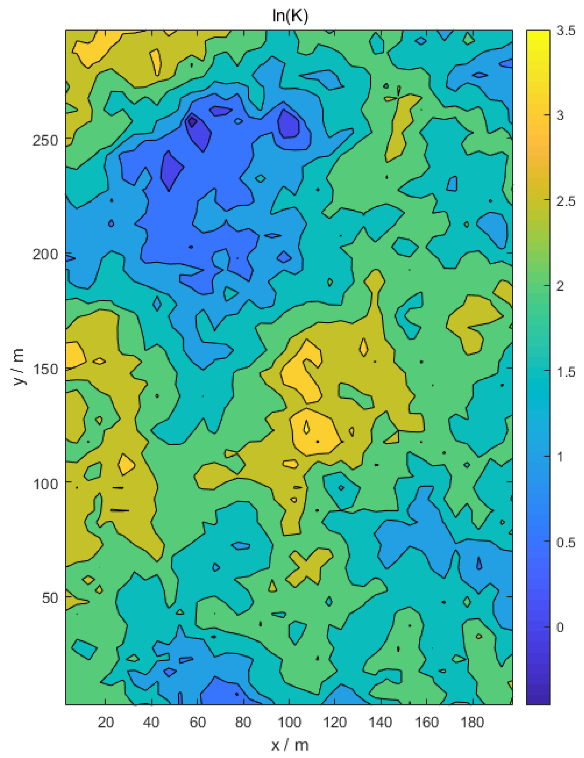
Step 2: Considering the uncertainty of site information, the random hydraulic conductivity field is generated by the LHS (Latin hypercube sampling) technique assuming hydraulic conductivity in a random process.
Step 3: Groundwater flow and the transport model are constructed and the concentration field library is obtained by Monte Carlo simulation. In the Monte Carlo simulation, each potential pollution source with unit mass-loading rate is calculated at each hydraulic conductivity realization.
Step 4: According to the weight of the pollution source, the concentration field is randomly selected from the concentration field library and the superposed pollution plume and covariance matrix are generated in combination with the mass-loading rate of the pollution source.
Step 5: Combined with the existing sampling data, the Kalman filter method is used to update the superposed pollution plume and the covariance matrix.
Step 6: According to the reduction in the overall uncertainty, new sampling data are selected sequentially using variance reduction with the Kalman filter method.
Step 7: Without adjusting the weight value of the pollution source, a linear programming model is adopted to identify the source mass-loading rate by using the existing sampling data.
Step 8: The superposed pollution plume is generated from the concentration field library based on the weight and mass-loading rate values prior to this step.
Step 9: Combined with the sampling data obtained prior to this step, the Kalman filter method is used to update the superposed pollution plume.
Step 10: Based on the morphological comparison of pollution plume, the weight value of the pollution source is updated by using the alpha-cut technique.
Repeat Step 4 to Step 10 until the weight value and overall uncertainty tends to be stable.
2.2. Groundwater Contaminant Transport Simulation
The contaminant transport, which is a complicated process in groundwater, may include advection, dispersion, diffusion, adsorption, and biodegradation. Prior to the simulation of the contaminant transport, the groundwater flow field should be figured out. The steady-state flow in a two-dimensional aquifer system can be expressed by the equation below.
where
Kij is the hydraulic conductivity,
H is the hydraulic head,
W is the volumetric flux per unit volume (positive for inflow and negative for outflow), and
x are the Cartesian coordinates.
The two-dimensional contaminant transport for conservative solute at a point source in groundwater can be given by the equation below.
where
is the porosity,
C is the contaminant concentration,
is the average linear velocity of groundwater flow,
Dij is the dispersion coefficient (a second-order tensor), and
R is the source or sink term.
The head distribution of the flow field can be estimated by Equation (1). Darcy’s law can be used to determine in Equation (3), which is shown below.
The temporal and spatial concentration distribution of released contaminants at a specified point can be simulated by Equations (1) and (2). In this study, MODFLOW and MT3DMS were used to simulate the groundwater flow and transport process, respectively.
2.3. Stochastic Simulation
In this study, the hydraulic conductivity field is assumed to be log-normally distributed and the semivariogram, which represents the log conductivity field’s spatial correlation structure, is an exponential model.
where
,
is the hydraulic conductivity,
is the variance of random
F, and
is the correlation length.
Given a probabilistic description of hydraulic conductivity, random field realizations are produced and served as input to numerical models. Realizations of hydraulic head and contaminant concentration are obtained as output from the model and the relevant statistics calculated.
In this study, the LHS technique (Latin hypercube sampling), which is a stratified sampling approach, was used to generate hydraulic conductivity realizations. The LHS approach is characterized by a segmentation of the assumed probability distribution into a number of non-overlapping intervals with each having equal probability [
35].
For each hydraulic conductivity realization, Equation (1) is solved and a steady state hydraulic head distribution is obtained. Equation (3) is then solved to get a velocity realization based on the head obtained from the hydraulic conductivity realization. A realization of the contaminant field is finally generated from the solution to Equation (2).
2.4. Concentration Field Library
However, repetitive calling of the simulation model (MODFLOW and MT3DMS) is requisite in the stochastic modeling and higher computation time is aggravated for the inverse problem. Therefore, in order to speed up the calculation, the concept of the concentration field library is proposed. The concentration field library is a library that stores the spatiotemporal concentration field for each potential pollution source of a unit mass-loading rate and is generated based on the principle of linear superposition, which requires the government equation to be linear. The following paragraphs describe the concept and implementation for the concentration field library.
Equation (2) can be rewritten as part of Equation (5).
The linear derivative operator
L(
C) represents the left side of Equation (4). Note that
Cj denotes the concentration field for the
jth potential source of the unit pollution mass-loading rate. Afterward,
Cj satisfies the following equation.
where
denotes the
jth potential pollution source of unit mass-loading rate (1 at the source
j and 0 at other grids).
In case of multiple pollution sources, based on the principle of linear superposition, the superposed concentration field
C (
) satisfies the equation below.
where
a is the number of potential pollution sources and
mj denotes the mass-loading rate of
jth potential source.
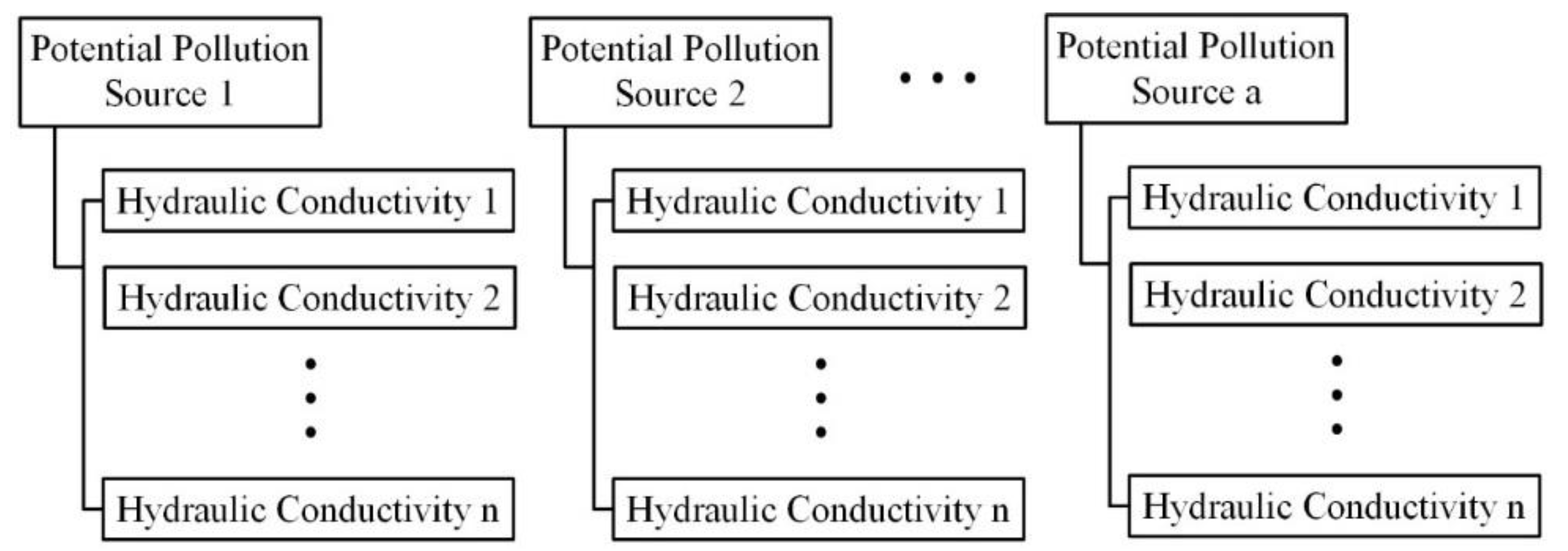
In this study, the potential pollution sources of the unit mass-loading rate are combined with hydraulic conductivity realizations (
Figure 2) and are regarded as model input to perform numerical simulations. After these processes, the concentration fields are stored in the concentration field library.
Given the weight and mass-loading rate of potential pollution sources ((
wj,
mj),
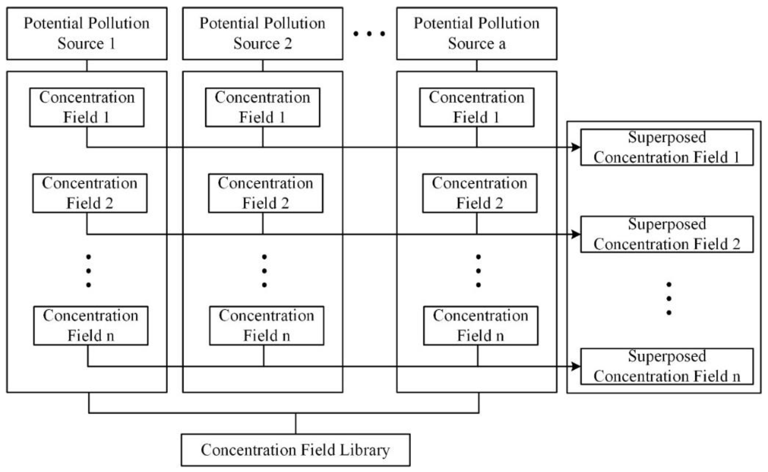
j = 1, …, a), the concentration field corresponding to each hydraulic conductivity realization is generated utilizing the following procedures (
Figure 3). First, according to the weight value of each pollution source, randomly select the concentration field from the
n concentration fields and assign the zero concentration field to unselected ones. Second, multiply the concentration fields by the mass-loading rate of the pollution sources. Third, superpose the concentration fields under the same hydraulic conductivity field. Lastly, we generate the
n concentration field realizations with the given weight and the mass-loading rate.
The mean concentration and the covariance matrix can be calculated based on the above realizations of the superposed concentration field. The average concentration
at location
i can be expressed by the equation below.
where
denotes the
kth concentration realization at location
i. In addition, the element (
i,
j) of the corresponding covariance matrix is shown in the equation below.
The resultant mean concentration and the covariance matrix are the prior estimates before any sample is taken. They would be used as the initial conditions in the Kalman filter method.
2.5. Kalman Filter Approach
Taking into account the uncertainty of hydraulic conductivity, which would be transferred to contaminant concentration uncertainty, the Kalman filter method combined with sampling data is used to estimate the concentration field so that the concentration of the estimated pollution plume is close to that of the true plume. In this study, the discrete static Kalman filter is chosen because time is not considered as part of the problem. The updated equations are below.
Update estimate with measurement z:
Update the error covariance:
where
K is the Kalman gain matrix,
P is the error covariance estimate,
is a vector of dimension
b that is an estimate of the concentration field, z is the vector of
l noise corrupted measurements,
H is the sampling matrix that contains zeros and ones (1: when a sample is taken at the specific location, 0: when a sample is not taken) with dimension of
. ,
r is the variance of sampling error, symbol—denotes prior estimate and + denotes posterior estimate,
b is the number of the computing node, and
l is the number of the sampling node.
However, due to the heterogeneity of the groundwater system, it is time-consuming and expensive to obtain the measured values. The efficient selection of observation points plays a crucial role in estimating the pollution plume. Considering that the Kalman filter is adopted as the estimation, the variance reduction is adopted to optimize the design of the monitoring network in this study.
To meet the requirements for the remediation of pollution plumes, the strategy of sequentially adding sampling points is considered until the total variance reaches a predefined threshold. Therefore, one single sampling point at a time is chosen sequentially to update the plume and error covariance matrix and the sampling matrix
H is a vector of dimension
b.
where the number 1 is located at the
jth sampling location. The sampling error covariance associated with the
jth location is denoted as
. The formula used to calculate the uncertainty measurement corresponds to each potential sampling location, which is shown in the equation below [
17,
19].
The term in the above equation represents the posterior total variance. The total variance reduction is achieved when reaches the maximum.
While the above-mentioned predefined threshold for total variance usually requires trial-and-error to get a reasonable value, for the ease of monitoring network design, we determined the operation of sequentially adding sampling points by judging whether the weight and mass-loading rate of potential sources tend to be stable.
2.6. Alpha-Cut Technique of a Fuzzy Set
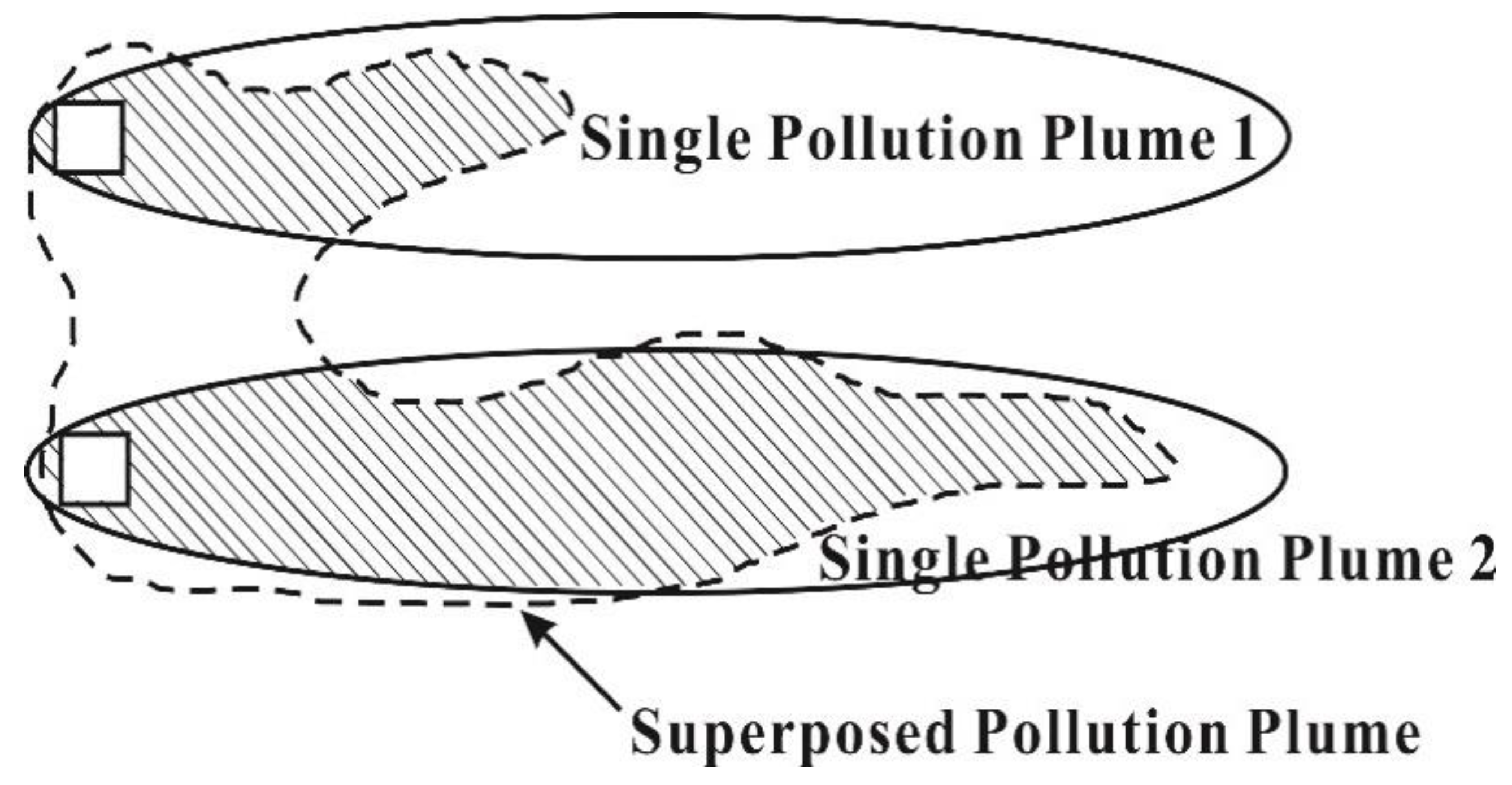
In the concentration field library, there are n non-superposed concentration fields for each potential pollution source and the resulting mean concentration field of these n concentration fields is named as a “single pollution plume”. If there are five potential pollution sources, it corresponds to five single pollution plumes.
An intuitive concept is that the single pollution plume, which is getting closer in morphology to the pollution plume, generally has a higher probability of being polluted. Therefore, each single pollution plume is compared with the updated superposed pollution plume and the similarity measurement between them will be used as the updated weight of the potential pollution source.
In order to measure the similarity, the pollution plumes are represented as fuzzy sets with membership functions and the membership function is defined as normalized concentration value s (all concentration values are divided by the maximum concentration value). The alpha-cut (
α-cut) technique of a fuzzy set provides the interval range corresponding to a specific value of membership function and is adopted in this study. Mathematically, the
α-cut technique is represented by the equation below [
18].
where
is a fuzzy set (the representative of the plume
), is the membership function (normalized concentration value), and
is the value of alpha. Several
α-cuts are considered such as five
α-cuts (
= 0.1, 0.3, 0.5, 0.7, 0.9).
Each
α-cut for the updated superposed pollution plume is compared with the corresponding
α-cut of each single pollution plume.
Figure 4 is the comparison of
α-cuts where the overlapping area of the two
α-cuts is shown in shade and the area of the overlapping areas
S (measure of similarity) are calculated. Afterwards, the global degree (
g) of similarity between two plumes is obtained by weighting the overlapping area by the
α-cut values and summing all the products (Equation (16)). Lastly, the degree of similarity between each single pollution plume and the updated superposed plume is normalized by the largest value of
g and is assigned as the updated weight values of each potential pollution source.
2.7. Linear Optimization Model
Using the method of contaminant plume morphological comparison, the location of the pollution source can be identified when the mass-loading rate of the pollution source is known. However, when the mass-loading rate is unknown, these pollution source identification problems would be more complicated. Afterward, the methods for modifying the pollution source mass-loading rate needs to be embedded in the aforementioned method. In this study, considering the computational efficiency, local search methods, which are not intelligent optimization algorithms, are adopted for modifying (also belongs to optimization) the mass-loading rate. A description of the optimization model for the mass-loading rate modification is presented below.
The decision variables in this optimization problem consists of the mass-loading rate for each potential pollution source and the objective function of the optimization model can be mathematically expressed below.
where
is the simulated concentration at sampling location
i,
is the measured concentration at sampling location
i, and
l is the total number of sampling locations.
The constraints for the optimization problems can be expressed by the equations below.
where
m is a vector of dimension
a,
is the mass-loading rate of the
jth potential pollution source, and
is the upper bound of the mass-loading rate of the pollution source.
represents the function that transforms the mass-loading rate of the pollution source into simulated concentrations via the physically-based model and can be obtained by performing arithmetic operations on the concentration filled library based on the principle of superposition.
The form of the objective function defined in Equation (17) is not compatible with linear optimization because it contains absolute values [
36]. It can be rewritten by using the equations below.
such that
Therefore, the constraints for the optimization problems with the decision variables are made up of Equations (18) and (19), Equations (21) and (22). In addition, the optimization problem defined above has only linear constraints and was solved by function linprog in MatLab.
4. Results and Discussion
4.1. Stochastic Modeling Analysis
Latin hypercube sampling (LHS) from a Gaussian distribution was applied to randomly generate the hydraulic conductivity realizations. The values of these parameters are described in
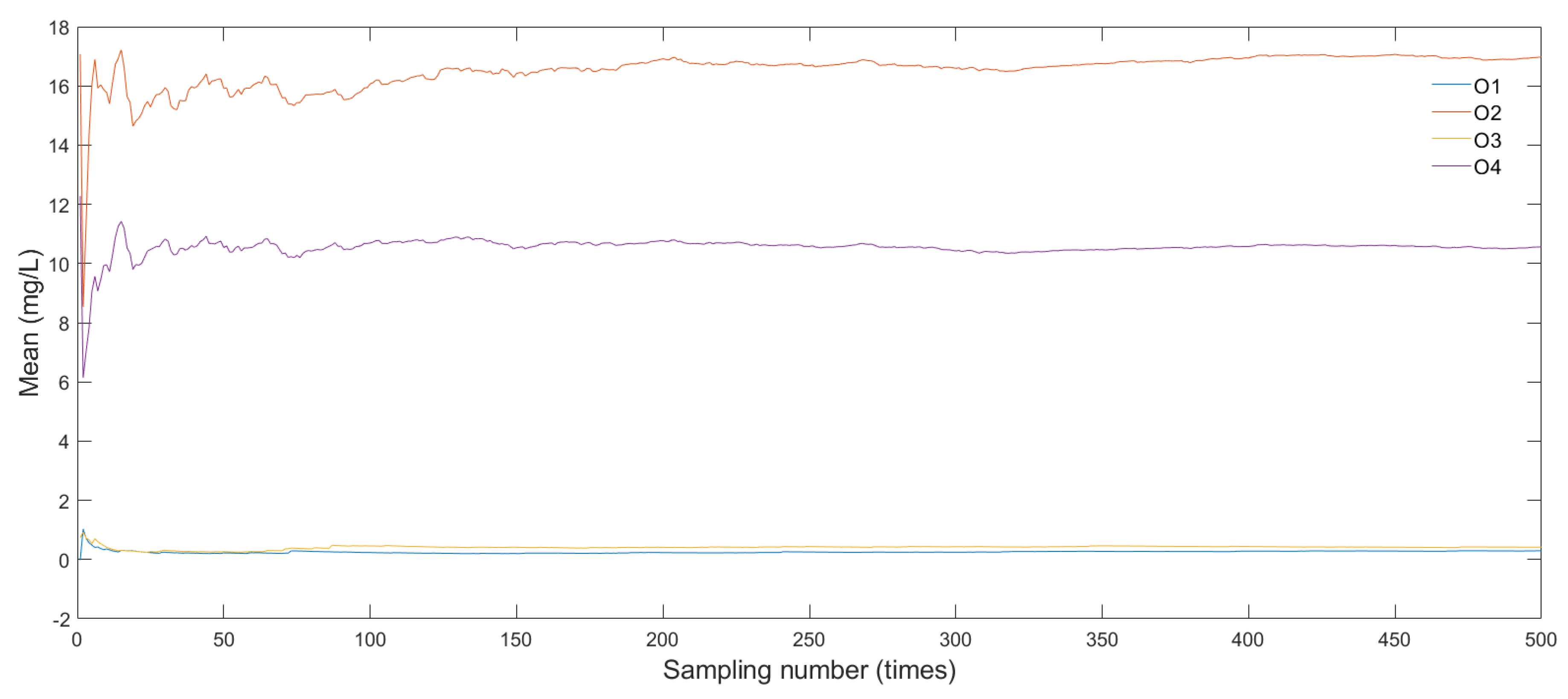
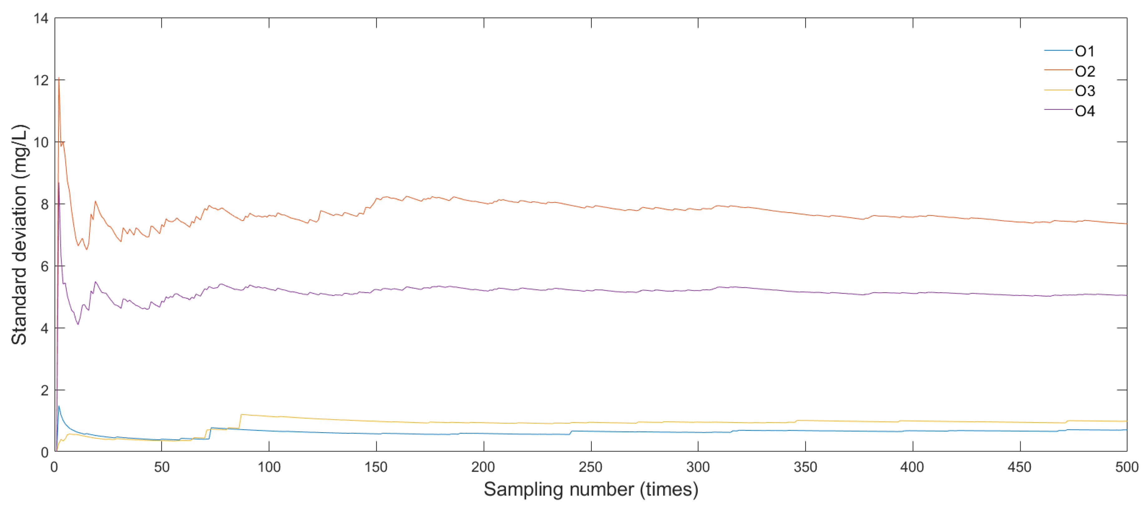
Section 3.1 and each realization was combined with five potential sources with a unit mass-loading rate to obtain the corresponding concentration individually. Therefore, the concentration field library that contains 2500 concentration realizations is built to choose to calculate the superposed pollution plume.
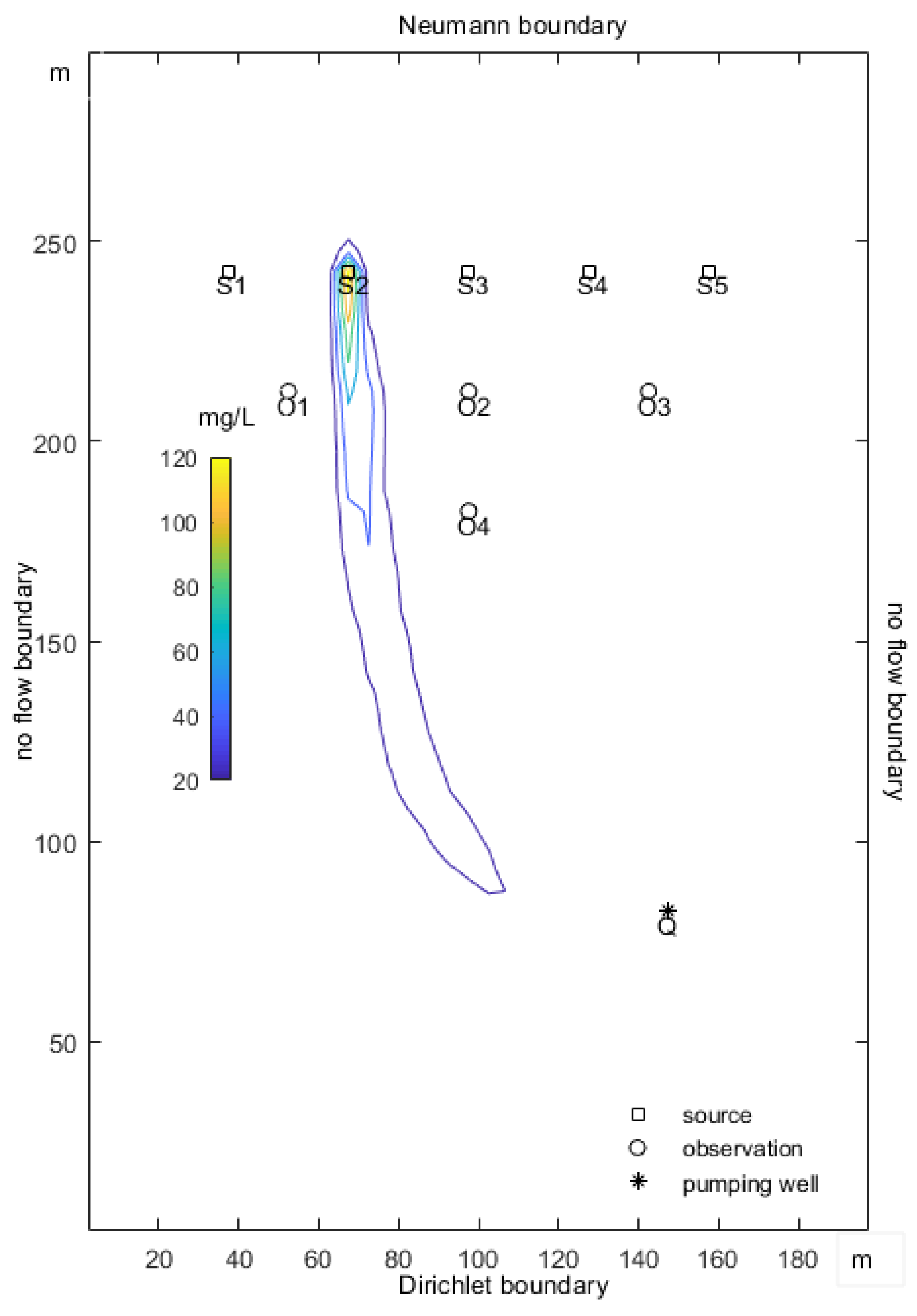
To test the validity and ergodicity of the concentration field library, the analysis of statistical characteristics (mean and standard deviation) at four virtual sampling points (O1–O4, in
Figure 5) is performed. In the course of analysis, these sampling data points are extracted from the 2500 realizations of the concentration field under the pollution sources with the weight of (0.7, 0.8, 0.9, 0.6, 0.9) and the mass-loading rate of 500 g/day.
Figure 7 and
Figure 8 are the iterative curves of mean and standard deviation for O1–O4, respectively. It can be seen that the mean value and standard deviation gradually reach a stable state with the increase of the sampling number and nearly converge after about 350 iterations (samplings). Therefore, the concentration field library obtained from LHS with 500 samplings is adequately satisfactory to be used for subsequent pollution source identification.
4.2. Pollution Source Identification
The illustrative application is solved with the proposed method discussed above. The parameters set for the proposed method are as follows. The initial weights of the pollution sources are set to (0.7, 0.8, 0.9, 0.6, 0.8), respectively. The initial mass-loading rates of the pollution sources are all set to 200 g/day. Four α-cuts (0.2, 0.4, 0.6, 0.8) for morphological comparison of pollution plume is adopted.
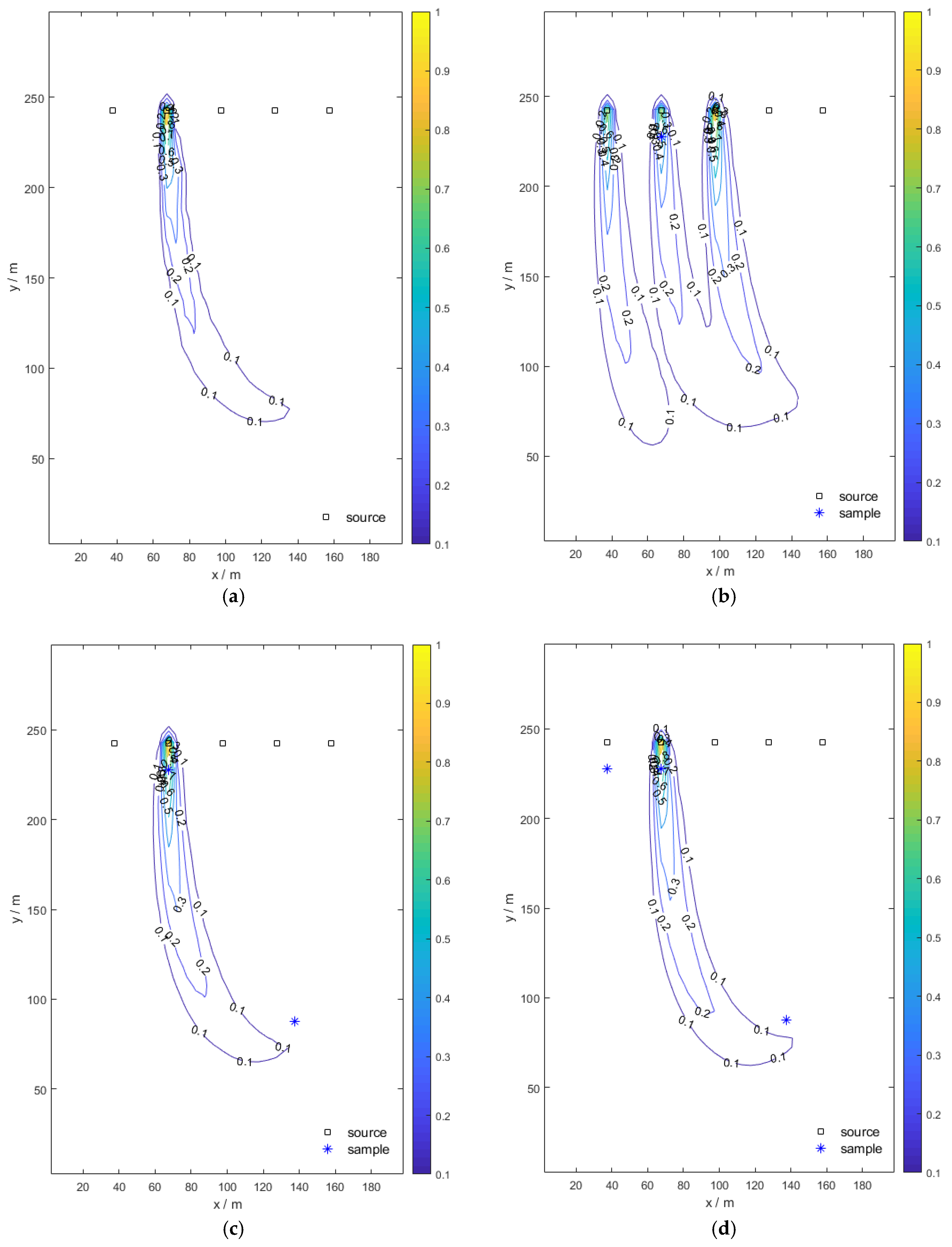
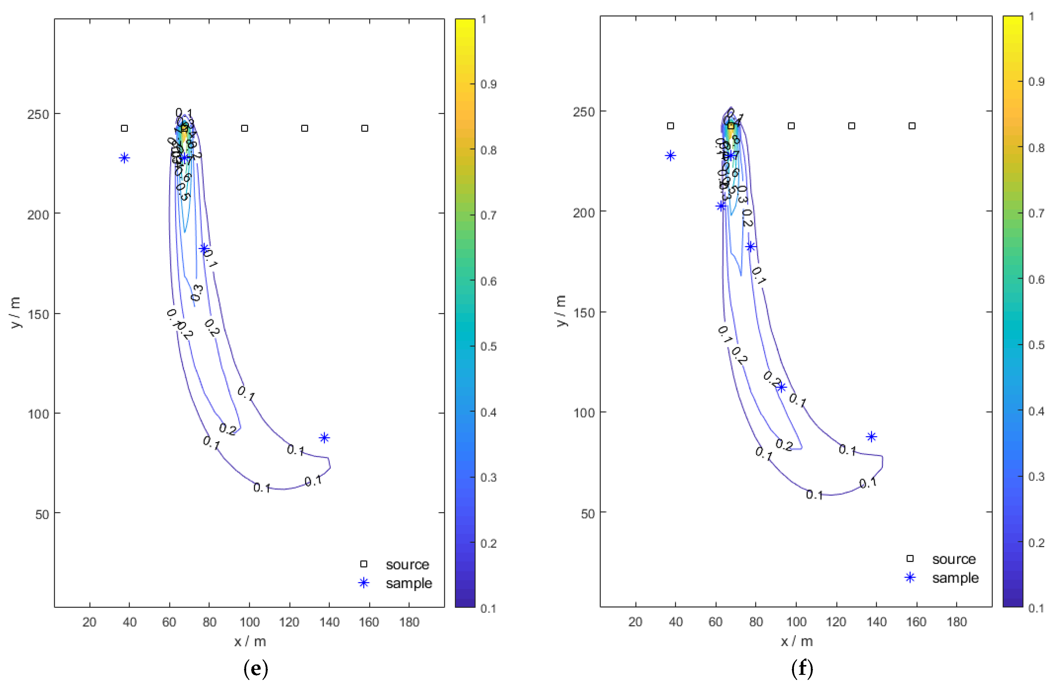
Figure 9 are the normalized contour maps of the pollution plume.
Figure 9a shows the true plume and
Figure 9b–f shows the pollution plume updated with 1, 2, 3, 4, and 6 monitoring sampling data, respectively. As the number of samplings increases, the shape of the pollution plume gradually approaches that of the true pollution plume.
Table 2 summarizes the identification results (mass-loading rates and weights of potential pollution sources) of the proposed method. In
Table 2, the weights and mass-loading rates of pollution sources tend to be stable after taking six samples. At this time, the corresponding weights of each potential pollution sources are (0, 1, 0, 0, 0), which exactly matches the actual situation and the corresponding mass-loading rates are (0.01, 530.64, 0.01, 0.01, 0.01), which the deviation of the mass-loading rate is about 6%. Note that the value of 0.01 is meant to prevent disturbances in solving the linear optimization problem for the mass-loading rates.
Therefore, it can be concluded that the proposed method is successful in identifying the true source location and characterizing the pollution morphology plume after the collection of six samples. The first sample is selected near the true pollution source for its high concentration value, the second sample is selected near the unknown pumping well to reduce this uncertainty, the third one is selected to exclude other potential pollution sources, and the other three samples are selected downstream of the true pollution source to characterize the plume.
4.3. Sensitivity Analysis
This section describes the results of the sensitivity analysis to gain insight into various aspects of the proposed method. The sensitivity analysis is performed for the illustrative problem and the parameters considered are the number and values of α-cuts, the initial weights, the initial mass-loading rate, and the heterogeneity of hydraulic conductivity field.
Three different settings of α-cuts are adopted for the sensitivity analysis and the results are shown in
Table 3. For comparison, keeping the former illustrative case as the first case, the second case omits the higher α-cut 0.8, and the third case uses the logarithmic α-cuts. It is shown that the α-cuts (0.2, 0.4, 0.6) get the worst results (the deviation is about 16%). The other two α-cuts settings get a similar result (6%~8%). This result can be demonstrated by the fact that more emphasis is given to the higher α-cuts, which may produce better results. Therefore, it can be concluded that this proposed method is sensitive to the setting of α-cuts to a certain degree.
The second parameter considered is the initial weight and the results are shown in
Table 4. The first case is the former illustrative case, which reduces the weight of the true pollution source to the lowest probability of 0.1 in the second case and the highest initial weight is only set to the potential pollution source farthest from true pollution source in the third case. It is shown that, in the last two cases, both need 11 sampling points to get the convergent result and the results is only slightly worse than first case. It can be concluded that the proposed method is less sensitive to the setting of initial weights.
The third parameter considered is the initial mass-loading rates and the results are shown in
Table 5. Assuming the first case is identical to the former illustrative case, the second case reduces the mass-loading rate of the true pollution source to 10% and the initial mass-loading rates in the third case are randomly selected. It is shown that all three cases get the same results at the same convergence speed (i.e., sampling points needed). It can be concluded that our proposed method is not sensitive to the setting of initial mass-loading rates.
The former three parameters are algorithm parameters while the last parameter taken into account for sensitivity analysis is the heterogeneity of hydraulic conductivity field.
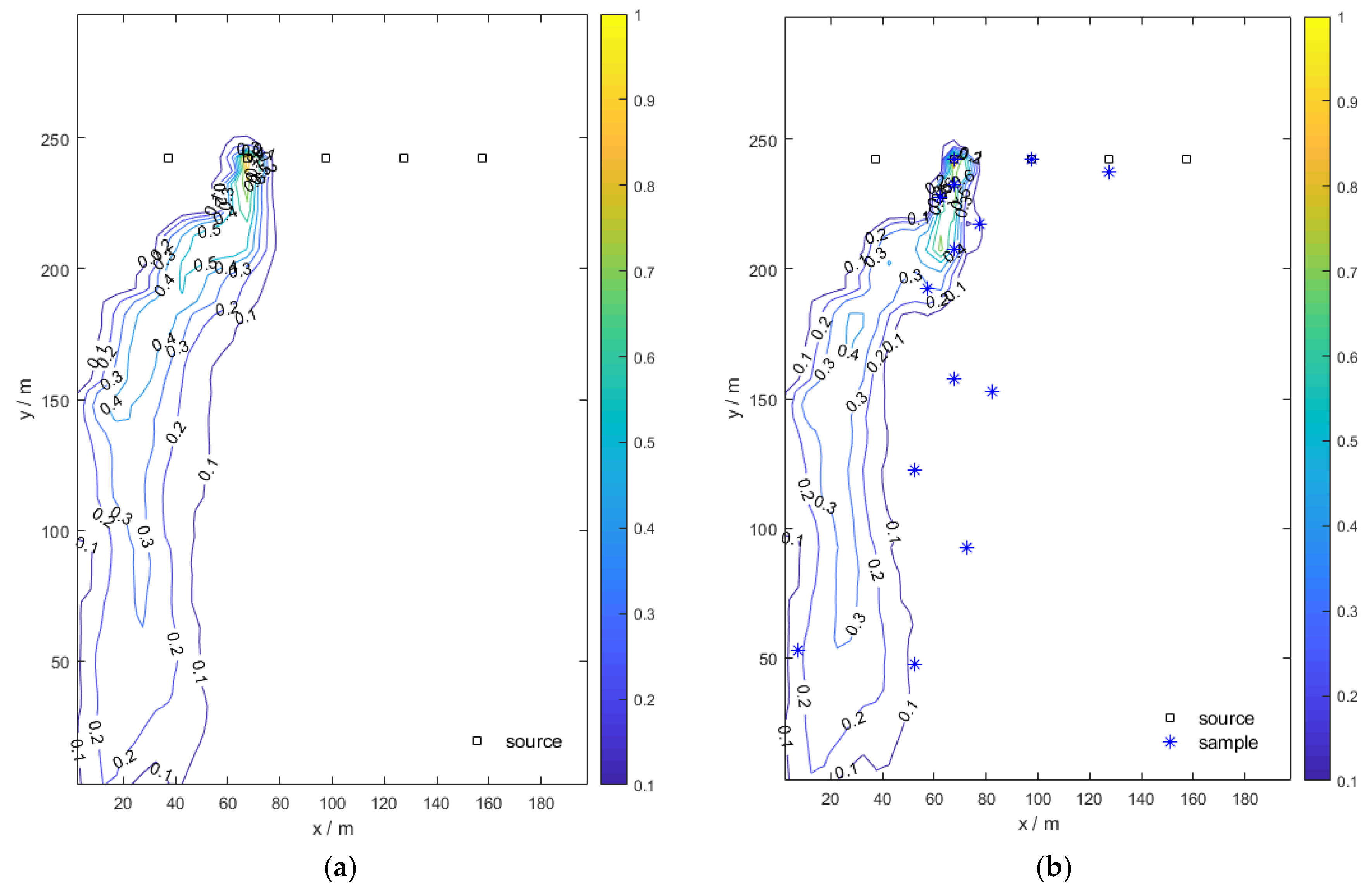
Table 6 is the sensitivity analysis results of the heterogeneity of hydraulic conductivity field. The small heterogeneity case denotes the former illustrative case, which increases the variance from 0.25 to 4.0 and keeps the mean and correlation length in the moderate heterogeneity case identical to those of the former case.
Figure 10a,b show the true plume and the pollution plume updated with 14 monitoring sampling data under moderate heterogeneity, respectively. In this case, we can observe that the shape of the identified pollution plume is close to the true plume (
Figure 10), but clear deviations appear at some locations.
In
Table 6, the stable weight of each potential pollution source under moderate heterogeneity is (0, 1, 0, 0, 0), respectively. According to the weight value, source 2 is determined and the actual mass-loading rate of source 2 is 422.32 g/day. Moreover, the deviation of the mass-loading rate under moderate heterogeneity is about 16%, which is higher than that of the medium heterogeneity case (6%).
Therefore, our proposed method is effective in identifying the true source location and characterizing the pollution morphology plume even under moderate heterogeneity condition (variance = 4.0), but the performance is less satisfied. More highly heterogeneity conditions (variance = 6.25, 9.0, 12.25, 16.0) are tested and our proposed method is completely invalid when tackling with highly heterogeneous field (variance = 16.0). It indicates that the proposed method can provide relative satisfied results for a homogeneous domain or a domain with a small and moderate heterogeneity, but it cannot validate the transport in the relatively high heterogeneous field. Therefore, our proposed method is sensitive to the heterogeneity of a hydraulic conductivity field.


