Flood Routing in River Reaches Using a Three-Parameter Muskingum Model Coupled with an Improved Bat Algorithm

Abstract

Design of hydraulic structures, flood warning systems, evacuation measures, and traffic management require river flood routing. A common hydrologic method of flood routing is the Muskingum method. The present study attempted to develop a three-parameter Muskingum model considering lateral flow for flood routing, coupling with a new optimization algorithm namely, Improved Bat Algorithm (IBA). The major function of the IBA is to optimize the estimated value of the three-parameters associated with the Muskingum model. The IBA acts based on the chaos search tool, which mainly enhances the uniformity and erogidicty of the population. In addition, the current research, unlike the other existing models which consider flood routing, is based on dividing one reach to a few intervals to increase the accuracy of flood routing models. Three case studies with lateral flow were considered for this study, including the Wilson flood, Karahan flood, and Myanmar flood. Seven performance indexes were examined to evaluate the performance of the proposed Muskingum model integrated with IBA, with other models that were also based on the Muskingum Model with three-parameters but utilized different optimization algorithms. The results for the Wilson flood showed that the proposed model could reduce the Sum of Squared Deviations (SSD) value by 89%, 51%, 93%, 69%, and 88%, compared to the Genetic Algorithm (GA), Particle Swarm Optimization (PSO) algorithm, Pattern Search (PS) algorithm, Harmony Search (HS) algorithm, and Honey Bee Mating Optimization (HBMO), respectively. In addition, increasing the number of intervals for flood routing significantly improved the accuracy of the results. The results indicated that the Sum of Absolute Deviations (SAD) using IBA for the Karahan flood was 117, which had reduced by 83%, 88%, 94%, and 12%, compared to the PSO, GA, HS, and BA, respectively. Furthermore, the achieved results for the Myanmar flood showed that SSD for IBA relative to GA, BA, and PSO was reduced by 32%, 11%, and 42%, respectively. In conclusion, the proposed Muskingum Model integrated with IBA considering the existence of lateral flow, outperformed the existing applied simple Muskingum models in previous studies. In addition, the more the number of intervals used in the model, the better the accuracy of flood routing prediction achieved.

1. Introduction

Flood routing is fundamental to the design of structural, as well as nonstructural, flood control measures [1]. Routing involves the calculation of changes in the magnitude, velocity, and shape of a flood wave, as a function of time at one or several points of the river [2]. There are two types of flood routing methods: Hydraulic and hydrological. Hydraulic methods have complex computations and are more data-intensive, but describe the complete flood wave profile, whereas hydrological methods are much simpler, but yield the flood hydrograph at the end of a reach [3,4,5,6,7]. The hydrologic methods need only the inflow hydrograph for a river reach. A common hydrologic method is the Muskingum method, which has several versions with parameters ranging from two to five. The two and three parameter versions of the Muskingum methods are more popular. In recent years, optimization methods, especially evolutionary algorithms, for estimating the Muskingum parameters have been popular [3]. A brief background of such algorithms is now given.

1.1. Background

The flood routing models mainly include two different types of modeling: the hydraulic and hydrologic models. The hydraulic model is usually developed in a one or two-dimensional domain. Full three water shallow models and two diffusive models were used for an urban site, and the results had the same difference with each other because of different representation of a numerical and hydraulic method in the model algorithm process [5]. Hunter et al [6] successfully set three explicit hydraulic models based on the inertia, diffusive, and shallow water models for flood simulation. The results indicated that the models with the shallow water equation were simple and could provide good accuracy, for the prediction of depth and velocity of the flood [5]. Dottori and Todini [7] evaluated two-dimensional models based on the diffusive wave for urban floods, and the results indicated that the model could simulate the overall phenomenon well. Kim et al. [8] evaluated the different meshes in diffusive models, to investigate the effect of different meshes on the flood hydrograph. Prestininzi [9] applied the diffusive models based on the impulsive wave for inundation areas, and the results showed the model could simulate the flood conditions even in complex topography, based on a good match of simulated results with the observed data. Aricò et al. [10] applied diffusive wave equation based on 2-D numerical models for a slow varying flood, and the results showed that the simulated depth of the flood had a relatively good match with observed data. Classical, explicit finite differences in the hydraulic models and simple Muskingum model were used to investigate the flood routing [11]. It has been reported that the applied numerical methods had numerical instability, for some case studies. As a result, the Muskingum model showed superior performance compared to the same applied hydraulic models [11]. It has been reported that the 2-D models could be developed, based on the availability of enough information about topography and topology. With this information, a 2-D hydraulic model could successfully simulate the flood characteristics for different urban conditions. In fact, digital maps helped to identify all the required information about the boundary conditions, and to differentiate between numerous transitions within the urban hydraulic modes [12].

In addition, it has been reported that the 2-D models had had trouble in application to particular cases under small water depths, especially when the status comes close to wet/dry boundary conditions, so that there is a need for specific algorithms for simulation [6]. Costabile et al. [13] reported that the main advantages of the one-dimensional model over the 2-D models for flood routing, are a simpler run process and low computational time where topographic data was unnecessary.

Fassoni-Andrade et al. [14] considered the development of a one-dimensional model based on the equation of hydrological models, which include the continuity equation and mass equation, such as the equation of the Muskingum models [14]. It was observed that one-dimensional flow routing inertial models, based on the explicit solution were superior to the other models. These models simplified the Saint-Venant equation, and the main advantages of these models were good simulated results with a simple structure. Singh and Arvamuthan et al. [15] applied two hydraulic models that were developed based on the Kinematic and diffusion waves, in addition, the results were compared to the Muskingum model for the flood routing. The results showed that the simulation of hydraulic models was dependent on the kinematic wave number, so that when the value of this parameter was not considered based on accurate computation, the results for the hydraulic model could be worse than hydrologic models. Costabile et al. [16] reported that 2-D models could overcome the limitation of 1-D models, when the case study characterized as unsteady flow in irregular topography. The reports showed that if the flow was not one dimensional for the urban hydraulic, the one-dimensional channel network should be used instead of a one-dimensional model. In addition, the results showed the significant difference between 1-D and 2-D models to simulate the velocity and depths.

However, the results showed that the complex nonlinear form characteristic, numerical stability, high computational time, and complexity in the run process of hydraulic models, meant that the simpler and more accurate models have high importance [13]. In fact, the hydraulic models need to measure the flow depth and discharge based on applying stream gaging. These models are known as complex models and difficult to use, whilst the hydrologic models need only to use the discharge data. In addition, the hydrologic models can be effective for the initial planning level, where the measuring system is undeveloped for accurate measurement [13]. For example, Chatila [17] simulated flood routing based on the Muskingum model and EXTRAN hydraulic model. The hydraulic model developed was based on finite difference. Both hydrologic models and hydraulic models, were applied on simple and compound channels for flood routing. The results revealed that the Muskingum model had achieved higher accuracy compared with the hydraulic model because of its flexibility in calibration, where even the river bed geometry was not considered for this model. It has been demonstrated that the Muskingum model could simulate the peak discharge, achieving a close fit with the actual one, compared to the hydraulic model. Furthermore, it has been reported that hydraulic models are dependent too many assumptions, such as reach geometry, channel slope, and flow velocity, which causes the application of some hydraulic models to be limited to the specific case studies.

The Muskingum model is a useful and important hydrological model, due to its high accuracy and simplicity. Hydrological models could be accomplished after estimating the value of parameters, on the other hand, hydraulic models are required to simulate the complex boundary hydraulic conditions that causes an increase in the computational time [17].

Therefore, this model was used as a model with free access, fast computation, highly accuracy, and low cost. Furthermore, it can be used as a good tool, instead of complex hydraulic models, for flood simulation. Additional background of the application of the Muskingum model and its integration with an evolutionary algorithm, will be presented and discussed hereinafter [18].

Under a two parameter Muskingum method, Luo and Xie [19] applied the immune clonal selection algorithm (ICSA) for flood routing in a river in China, and found that the algorithm had faster convergence than the GA and PSO; and routed discharges had a high correlation with observed discharges.

Geem [20] obtained the two parameters of Muskingum method using a harmony search algorithm (HAS) for the Wilson flood in the USA, and obtained less root mean square between the predicted and observed discharges, than for GA and PSO, and less computational time.

Nelder-Mead simplex algorithm (NMSA) was considered for flood routing, and a case study in the USA [21]. The parameters of the Muskingum model were considered as decision variables, and the results indicated that the RMSE (root mean square error) based on NMSA decreased by 20%, compared to the genetic algorithm [21].

Karahan et al. [22] applied a hybrid of GA, HAS, and nonlinear programming to a three-parameter Muskingum method for flood routing in a river, and found the hybrid algorithm more accurate.

Orouji et al. [23] used a genetic programming algorithm (GPA) for flood routing by the Muskingum method, and showed that GPA was more accurate than GA and PSO. The Muskingum model by 4 parameters was considered under different case studies [23].

Four parameters were considered as decision variables, and the results indicated that the model based on the considered parameters with the genetic algorithm decreased the RMSE and mean absolute error (MAE) by 20% and 25%, respectively, compared to the nonlinear programming methods [24].

The hybrid PSO and harmony search algorithm was considered for flood routing [25]. The results indicated that the new hybrid method could increase the convergence velocity of the harmony algorithm, and decreased the error indexes, RMSE, and MAE, compared to the simple harmony and particle swarm algorithm.

Ouyang et al. [26] applied a hybrid of PSO and GA for Muskingum flood routing and showed that the hybrid algorithm was faster, and more accurately predicted the peak discharge and time to peak.

Under the three-parameter Muskingum method, Geem [27] found the harmony algorithm (HA) to have higher convergence than PSO and GA. Under the four-parameter Muskingum method, the Frog Leaping Algorithm (FLA) was found to have a lower computational error, than PSO and GA [28]. Niknazar and Afzali [29] used an improved Honey Bee Algorithm (IHBA) to optimize three parameters of the Muskingum method, and found it to be superior to GA and PSO.

Using an Invasive Weed Optimization Algorithm (IWOA) for parameter optimization, Hamedi et al. [2] found the five-parameter Muskingum method to be more accurate than the four-parameter version. With PSO for parameter estimation, Moghadam et al. [30] found the four-parameter Muskingum method to be more accurate, than the three-parameter Muskingum method with GA and linear programming.

Using the gravitational search algorithm for parameter optimization, Kang et al. [31] found the four-parameter Muskingum method to be accurate for flood routing. Flood routing for a case study in China based on real code genetic algorithm was considered [3], and the results indicated that the four-parameter Muskingum model based on genetic algorithm decreased the RMSE and MAE of the two- and three-parameter Muskingum models.

Barati et al. [21] applied different kinds of GPA to the four-parameter Muskingum method for flood routing, and found the fixed genetic programming to be more accurate. For flood routing using the Muskingum-Cunge method, Wang et al. [23] found PSO to yield better results than GA.

In 2018, Lee [32] developed and applied an advanced Muskingum flood routing model by considering continuous stream flow, utilizing weighted inflow. Several statistical indicators have been used to evaluate the performance of the suggested model. The proposed model provided acceptable results, compared to those obtained from previous studies. The results showed that the vision corrected algorithm (VCA) had experienced a relatively small error index compared to the GA, PSO, and nonlinear programming models, for different flood case studies.

The literature review showed that the evolutionary algorithm has a high ability for obtaining the parameter values of the Muskingum model, but some algorithms have limitations, such as trapping in local optimums, slow convergence velocity, or insufficient accuracy for the simulation [33]. For example, the GA can trap in the local optimums or the PSO may have an immature solution due to fast convergence [1,27]. Some evolutionary algorithms have many random parameters, and accurate determination of these parameters is difficult. Thus, the improvement of previous algorithms or definition of new algorithms is necessary.

1.2. Problem Statement

Flood routing is nonlinear and multimodal, with noise. The most widely used model for flood routing is the Muskingum model. One of the main components of the Muskingum model procedure, is the inclusion of a particular number of parameters ranging between two and five, which have to be estimated based on the case study characteristics to be able to accurately route the flood. There are different procedures to estimate the Muskingum model parameters. Actually, the better the estimation of the parameters’ value, the better the prediction of the flood routing characteristics achieved [33,34,35,36,37]. Having an optimization algorithm that is able to optimize the value of these parameters, whether two or three, is needed to enhance the ability of the Muskingum model to identify the flood routing characteristics. Thus, a robust algorithm that leads to the global optimal solution is needed. Bats exhibit a mysterious behavior that has long been attractive. They are able to orientate themselves to their surroundings and food acquisition, without depending on their eyesight. Bats consistently emit echolocation signals. Through analyzing the returning echoes in the auditory system, bats can distinguish their environment and find preys. By continuously watching and concentrating on the abilities of bats, scientists have suggested different bat-inspired algorithms (i.e., bat algorithm (BA) and bat intelligence (BI) algorithm) for the solution of optimization problems [33,34]. Bozorg-Hadad et al. [35] used BA to optimize the use of a repository to reduce hydroelectricity energy shortage. This algorithm has been shown to have a faster convergence, than GA and PSO. Ahmadinafar et al. [36] used a hybrid BA to exploit a 10-repository system to increase energy production, which reduced computational time compared to other evolutionary algorithms. Studies have shown that BA is a powerful method but it has weaknesses, such as trapped in the local optimum or premature convergence [37,38]. Thus, it needs to be improved.

1.3. Objective

In the light of the above, the use of Muskingum model showed its success when applied in flood routing prediction, but it has a few limitations. For example, it cannot be used for the complex boundary condition. In addition, one of the weaknesses of the model is the consideration of the lateral flow. In fact, most of the previous researches ignore the lateral flow while using the simple Muskingum model. Therefore, if lateral flow exists and has high volume, the Muskingum model simulates the flood without consideration of lateral flow [23,24,25,26,27,28,29,30,31], and hence, the achieved accuracy is relatively low. In fact, simplification of the Muskingum equation was a reason to omit the effect of lateral flow for flood routing, whilst there is lateral flow in the reach when the flood happens in nature. Although, there are a few number of references considering the lateral flow, some of them are limited to specific case studies with the low flow lateral condition and using Muskingum models with a simple structure [39,40,41,42].

Limited studies showed that the consideration of the lateral flow, with the help of hydraulic models, could simulate the actual situations that close to the real conditions [12]. Osolivan et al. [17] reported the disadvantages of the hydraulic models for flood routing in the floodplain. Their reports showed that the initial and boundary conditions, and the resistance characteristics of main channels in the floodplain, are neccessary for the hydraulic modeling.

The present study develops the new Muskingum model for flood routing considering lateral flow. In addition, the Muskingum Model has been coupled with a new Improved Bat Algorithm (IBA), to optimize the estimation of the three-parameter Muskingum model.

The objective of this study, was to couple the three-parameter Muskingum method (TPMM) with an improved bat algorithm (IBA) for flood routing, with a multi-reach method and consideration of lateral flow. Citing easy trapping in the extremum for bat algorithm, an improved bat method is suggested and used to simulate flood routing. Chaos search tool is defined to enhance the uniformity and ergodicity of the population. Adapting weight is defined to balance the local and global search tools, for the bat algorithm. One of the advantages of the new bat algorithm is related to decreasing the search range, based on dynamic contraction.

The innovation of the study is the use of a new bat algorithm for flood routing lateral flow. Moreover, whilst previous studies usually considered one reach for flood routing without lateral flow, the present study compared the effect of dividing a river into different reaches on flood routing, and the prediction of peak discharge.

2. Materials and Methods

2.1. Flood Routing

The Muskingum method of flood routing is based on the continuity equation and a storage-discharge relation [30]. The present study considers the lateral flow for the flood routing for the case studies based on a ration of inflow rate $O_{lateral}=\beta I_t$, while the other studies do not consider the effect of lateral flow for flood regime, and thus it adds one term to the equation of the Muskingum model with three parameters. If $\beta$ coefficient equals to zero, the lateral flow has not been considered for the flood routing.

$$\frac{d{s}_t}{dt}=O_t-\left(1+\beta \right)I_t$$

(1)

$$S_t=K\left[X\left(1+\beta \right)I_t+\left(1-X\right)O_t\right]$$

(2)

where $O_t$ is the output flow at time t, $I_t$ is the input flow at time t, $S_t$ is the storage at time t, $\frac{d{s}_t}{dt}$ is the storage time variation at time t, K is the time coefficient of storage, and X is the weighting factor showing the effect of input and output flows on storage.

Equation (2) expresses a linear relation between storage, and input and output flows. However, a non-linear has also been presented as:

$$S_t=K{\left[X\left(1+\beta \right)I_t+\left(1-X\right)O_t\right]}^m$$

(3)

where m is an exponent. Using Equations (1) and (3), one can obtain [21]:

$$O_t=\left(\frac{1}{1-X}\right){\left(\frac{S_t}{K}\right)}^{\frac{1}{m}}-\left(\frac{X\left(1+\beta \right)}{1-X}\right)I_t$$

(4)

$$\frac{\Delta S_t}{\Delta t}=-\left(\frac{1}{1-X}\right){\left(\frac{S_t}{K}\right)}^{\frac{1}{m}}+\left(\frac{1\left(1+\beta \right)}{1-X}\right)I_t$$

(5)

Using $S_t,\Delta S_t$, the storage later can be expressed as:

$$S_{t+1}=S_t+\Delta S_t$$

(6)

Flood routing can be done using the following steps:

• Consider initial values for parameters K, X, $\beta$, and m and enter them into the optimization algorithm, in the form of initial population.
• Calculate the storage based on Equation (3), assuming the equality of input and output flow.
• Calculate the change in storage relative to time, based on Equation (5).
• Calculate the storage based on t + 1, according to Equation (6).
• Calculate the output flow at t + 1, based on Equation (4).
• Repeat steps 2 to 5.

2.2. Optimization of Multi-Reach Muskingum Coefficients

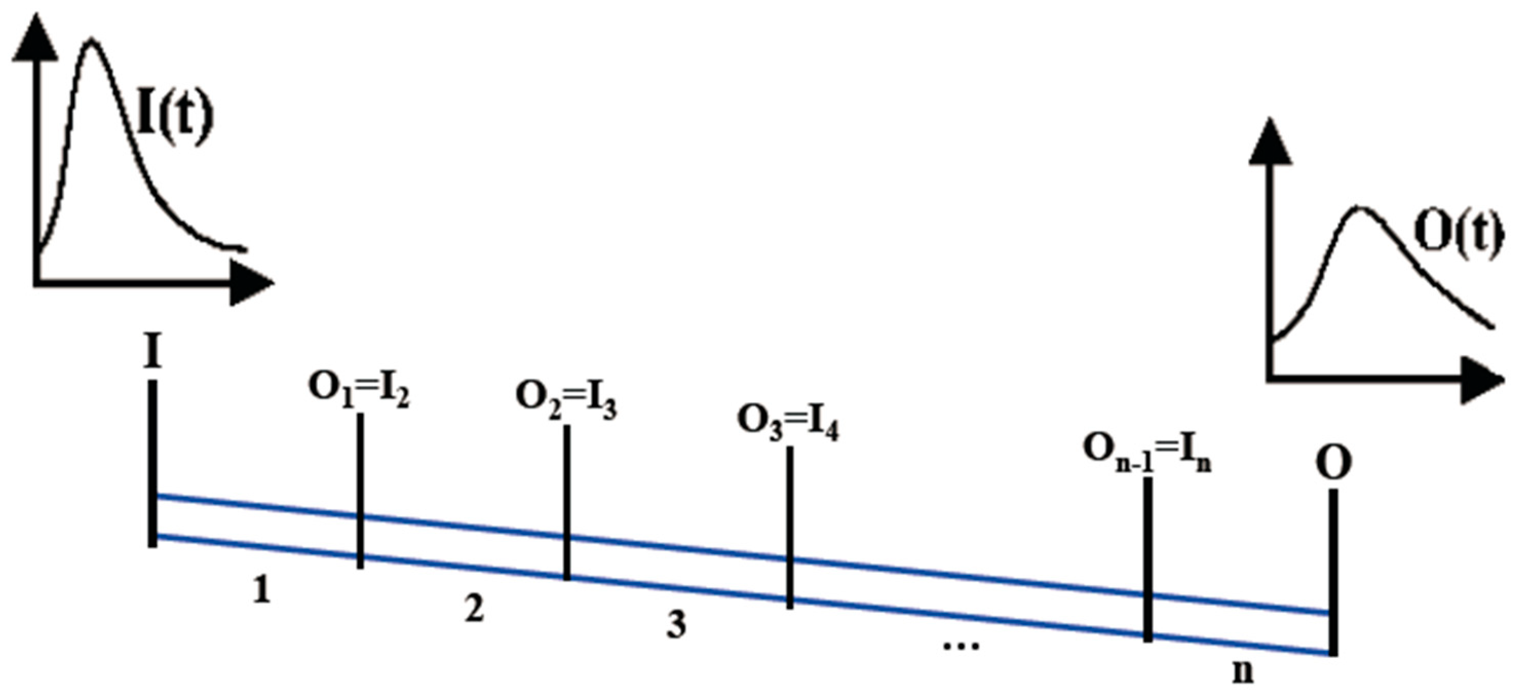
The multi-reach Muskingum method is introduced to enhance the accuracy of the Muskingum method. The river under study was divided into several smaller reaches, and for each reach, routing was done separately. In other words, for each reach, parameters X, K, β, and m were calculated separately, and the output hydrograph was obtained based on the input flood hydrograph and the assumed values of X, K, β, and m for the first reach [3,21,28,31]. This output hydrograph was considered as the input hydrograph for the second reach, and so on. For the second reach, the assumed values of X, K, β, and m were used, and the output hydrograph was calculated. This process was repeated for all the reaches, until the output hydrograph of the last was obtained. By comparing the computed hydrograph with the observed hydrograph, the error was calculated, and to reach the minimum error, Muskingum coefficients were optimized at all reaches. Figure 1 shows the division of the river into several reaches.

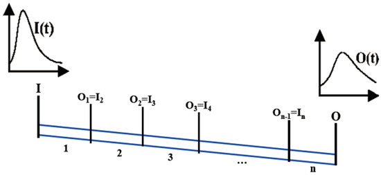
Figure 1. Discretization of the river stream.

2.3. BAT Algorithm

Bat algorithm (BA) is based on bat sound reproduction and sound reflection. The difference in loudness that comes from the surrounding environment, allows the bat to identify the barrier from food. Bats produce very high sound pulses and listen to their return from the objects around. Each pulse remains only for a few milliseconds. BA is based on the following assumptions [30,39,40,41]:

• All bats have a high ability to receive sound, so that they can detect food after producing loud sounds.
• Bats fly randomly at a velocity at place y_l, capable of producing sound with f_min frequency and $\lambda$ wavelength. The sound produced by bats also has loudness $A_0$.
• The loudness of sound, of the bats ranges from $A_0$ to $A_{\min }$.

Each sound produced by the bat has a pulse rate (r), between 0 and 1. The sound frequency speed and position of the bats are updated as:

$$f_l=f_{\min }+\left(f_{\max }-f_{\min }\right)\times \beta$$

(7)

$$v_l\left(t\right)=\left[y_l\left(t-1\right)-Y_{\ast }\right]\times f_l,t=1,2,\dots T$$

(8)

$$y_l\left(t\right)=y_l\left(t-1\right)+v_l\left(t\right),t=1,2,\dots ,T$$

(9)

where $f_l$ is the frequency of sound of bats, $f_{\min }$ is the minimum frequency, $f_{\max }$ is the maximum frequency, $\beta$ is the random coefficient between 0 and 1, $v_l\left(t\right)$ is the velocity of the bat, $Y_{\ast }$ is the best position of the bat, $y_l\left(t\right)$ is the position of the bat, and T is the number of periods evaluated.

The following equation is used for local search in the bat algorithm:

$$y\left(t\right)=y\left(t-1\right)+\epsilon A\left(t\right),t=1,2,\dots ,T$$

(10)

where $\epsilon$ is the random variable between −1 and 1, and $A\left(t\right)$ is the loudness of sound. Loudness and pulse rates are updated, according to each stage of the iteration. For example, zero sound loudness means that the bat has found its prey and has temporarily stopped the search.

$$r_l^{t+1}=r_l^0\left[1-\exp \left(-\gamma t\right)\right]A_l^{t+1}=\alpha A_l^{t+1}$$

(11)

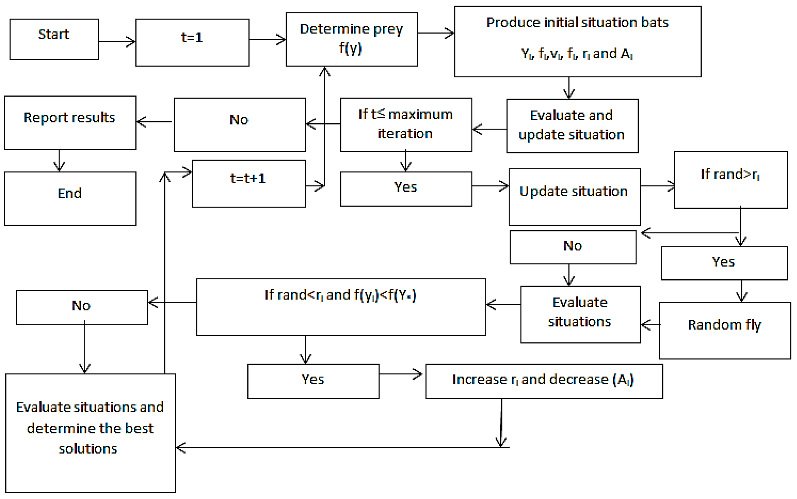
where $\alpha$ and $\gamma$ are fixed as constant coefficients. For any value of $\alpha$ between 0 and 1, and $\gamma$ greater than zero, $A_l^t\to 0$ and $r_l^t\to t_l^0$ are true. Figure 2 shows the mathematical procedure of the bat algorithm. In addition, it should be noted that the random walk is considered as a parameter for the local search, for the bat algorithm.

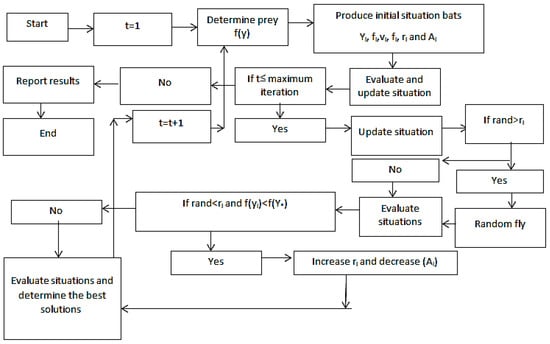
Figure 2. The flow chart of the bat algorithm.

2.4. Improved Bat Algorithm (IBA)

The initial arrangement for the initial version of the BA is defined randomly, and it can be a reason for the uneven distribution that causes premature convergence. The chaos is a technique for improving different algorithms, where the basic idea is related to the exchange of members in the range of (−1,1). The logic mapping function is used for modulating the algorithms. Then individuals are inserted into the chaos sequence, so that it should satisfy the chaos variable space. Then, linear transformation is used to return the members to the corresponding position. The convert space is shown based on following mathematical equation:

$$L_i=\frac{2\left(x_i^a-a\right)}{\left(b-a\right)}-1$$

(12)

where $x_i^a$: the initial position of the members.

The following equation is used to show the logic mapping function:

$$L_{i+1}=1-2\times L_i^2$$

(13)

Then, the elements and values are returned to the corresponding position by the following linear transformation:

$$y_i^0=\frac{1}{2\left(b-a\right)}{L}_i+\frac{1}{2\left(b+a\right)}$$

(14)

Furthermore, adapting weight is applied to the bat algorithm to have a good balance between global search ability and local search ability.

$$y_l^t=w\left(t\right)·y_l^{t-1}+v_l^t$$

(15)

The weight is computed based on the following equation:

$$w\left(k\right)=\frac{w_{\max }·\left(w_{\max }-w_{\min }\right)·\left(T_{\max }-k\right)}{T_{\max }}$$

(16)

$w_{\max }$: the initial weight, $w_{\min }$: the final weight, and k: the current iteration number.

The final level is related to the application of dynamic contraction, for adjusting the convergence speed:

$$\begin{array}{l}{y}_{\min ,i}=\max \left\{y_{\min ,i},x^{\ast }-rand\times \left(y_{\max ,i}-y_{\min ,i}\right)\right\}\\ y_{\max ,i}=\min \left\{y_{\max ,i},x^{\ast }-rand\times \left(y_{\max ,i}-y_{\min ,i}\right)\right\}\end{array}$$

(17)

where $y_{\min ,i}$: the lower bound position, and $y_{\max ,i}$; the upper bound position.

The algorithm functions using the following steps:

• Adjust the random parameters for the algorithm, such as loudness, pulsation rate, frequency, and other parameters.
• The individual position is computed using Equations (13)–(15), and then the objective function is computed for each member, and the best solution is considered as $Y_{\ast }$.
• The frequency and velocity are updated using Equations (7) and (8), and the position is computed using Equation (17).
• The randomness value is compared with r_l, and if r_l is less than the randomness value, the distribution of the best position is acted based on 0.01 times the random disturbance.
• The local search is considered for this level. If the loudness is less than rand, the loudness should be updated and the pulsation rate should be improved using Equation (12).
• Compute the objective function and change the range using Equation (16).
• The convergence criterion is checked and if it is satisfied, the algorithm finishes or else the algorithm goes to step 2.

2.5. Genetic Algorithm (GA)

In GA, the initial version of the population is composed of different solutions [40]. During an iterative process, subsequent populations are generated to improve the objective function. At each stage, some members from the current population are selected to generate individuals or children of the next generation, based on the fact that the likelihood of selecting people with better performance than others is more likely [41]. The selected individuals produce the next population based on two genetic operators, composition and mutation. The following equations can be used for the composition operator [33].

$$Po{p}_i^{new}=\alpha Po{p}_i^{old}+\left(1-\alpha \right)Po{p}_j^{old}$$

(18)

$$Po{p}_{new}^j=\alpha Po{p}_j^{old}+\left(1-\alpha \right)Po{p}_i^{old}$$

(19)

where $Po{p}_i^{new}$ is the i-th child, $Po{p}_i^{old}$ is the i-th parent, $Po{p}_j^{old}$ is the j-th parent, $Po{p}_{new}^j$ is the j-th child, and α is a coefficient between 0 and 1. Moreover, mutation is based on the following equation:

$$Po{p}_{i,j}^{new}=Va{r}_{i,j}^{low}+\beta \left(Va{r}_{j,i}^{hi}-Va{r}_{j,i}^{low}\right)$$

(20)

where $Va{r}_{i,j}^{low}$ is the lower limit of the i-th gene in the j-th chromosome, $Va{r}_{j,i}^{hi}$ is the upper limit of the i-th gene in the j-th chromosome, and $\beta$ is a random coefficient between 0 and 1. In composition, the production of both new individuals is done by changing the gene. The mutation operator is used for the change in chromosomes and transforming their genes to create diversity in the population.

2.6. Particle Swarm Algorithm (PSO)

Initially, the process starts with a particle set. Each particle is considered as a random solution. In the next step, searches are performed sequentially to achieve the optimal answer. The i-th particle is associated with a position in an s-dimension space, where the value of s shows decision-making variables of the problem [42]. The values of s variables, which determine the positions of particles are a possible solution for the optimization problem. Each particle i is completely determined by three vectors. Vector X_i is the current position of the particle, Y_i is the best position where the particle is iterated, and the vector of the particle velocity is shown by $V_i$. Then the particle position and particle velocity vector are updated as:

$$V_i^{iter+1}=w{V}_i^{iter}+c_{1}rand\left(Y_i^{iter}-X_i^{iter}\right)+c_{2}rand\left(Y_{\ast }^{iter}-X_i^{iter}\right)$$

(21)

$$X_i^{iter+1}=X_i^{iter}+V_i^{iter+1}$$

(22)

where $V_i^{iter+1}$ is the new velocity of the particle, the personal learning coefficient $c_2$ is the global learning coefficient, $Y_{\ast }^{iter}$ is the best solution among the solutions, and $X_i^{iter+1}$ is the new position of the particle. Moreover, w is the coefficient of inertia.

Indices of Error Measurement

1. The sum of squared deviations (SSD): SSD index is used as the objective function in the present study. The index calculates the total of squared deviations between observed and real discharges [28,42,43,44,45,46]:

$$Minimize(SSQ)={\displaystyle \sum _{t=1}^n{(O_{bt}-O_{st})}^2}$$

(23)

where $O_{obt}$ is the observed discharge, $O_{st}$ is the simulated discharge, and n is the number of data.

2. The sum of absolute deviations (SAD): SAD is the total sum of total deviations between observed and predicted discharges [20,30]:

$$Minmize\left(SAD\right)={\displaystyle \sum _{i=1}^n\left(O_{bt}-O_{st}\right)}$$

(24)

3. Error of Peak discharge (EP): EP index measures the difference between predicted and observed discharges [43,44,45,46].

$$E{Q}_p=\frac{\left|O_{observed}^{peak}-O_{routed}^{peak}\right|}{O_{observed}^{peak}}$$

(25)

4. Error of time to peak (ETP): The ETP index measures the difference between predicted and observed time differences of discharge [24,37,38].

$$E{T}_p=\left[T_{observed}^{peak}-T_{routed}^{peak}\right]$$

(26)

$T_{observed}^{peak}$ is the observed discharge, and $T_{routed}^{peak}$ is the time related to the routed discharge.

5. Mean absolute relative error (MARE): The mean of the relative error between observed and predicted discharges:

$$MARE=\frac{1}{N}{\displaystyle \sum _{i=1}^n\frac{\left(Q_t^{observed}-Q_t^{routed}\right)}{Q_t^{observed}}}$$

(27)

N is the number of data.

6. Varex Q (Variance index): This indicator shows the proximity of predicted and observed hydrographs with each other.

$$VarexQ=\left[1-\frac{{\displaystyle \sum _{i=1}^N\left(O_t^{observed}-O_t^{routed}\right)}}{{\displaystyle \sum _{i=1}^N\left(O_t^{observed}-O_{mean}^{observed}\right)}}\right]\times 100$$

(28)

$O_{mean}^{observed}$ is the observed average discharge. The closer the coefficient is to one, the more accurate the ability to predict the flood will be.

7. The agreement index (d) based on follow equation, shows the performance of the model well, so that the value of index can change from 0 to 1 [45,46].

$$d=1-\frac{{\displaystyle \sum _{i=1}^N{\left(O_i^{observed}-O_i^{routed}\right)}^2}}{{\displaystyle \sum _{i=1}^N\left(\left|O_i^{routed}-{\overline{O}}_i^{observed}\right|+\left|O_i^{observed}-{\overline{O}}_i^{observed}\right|\right)}}$$

(29)

${\overline{O}}_i^{observed}$: average of observed data.

3. Results and Discussion

This paper considered three case studies for flood routing. Two case studies were considered as bench problems, which have been used by different researchers using many methods for flood routing (Wilson and Karahan floods), and one case study was related to a river in Myanmar that had an important flood. The Wilson flood is considered as an important case study and different researchers tested different algorithms on this case study [2,3,28,29,30], and thus a comprehensive study can be considered for this case study. The Karahan flood is considered as one of the case studies that have been investigated by different researchers as a benchmark problem [28,29,30,31,35].

3.1. Wilson Flood

Wilson Flood [44] is one of the most important benchmark applications, to investigate the performance of the Muskingum model and other hydrologic models. In fact, this flood pattern was generated under experimental conditions. Different mathematical models were examined using this flood data pattern, which received great attention from researchers in examining their models.

The data was extracted from Wilson [44]. This information includes single peak inflow and outflow hydrographs with lateral flow. In addition, the applied algorithms in this research consider the lateral flow, although as shown in Table 4, previous researches have ignored the lateral flow because of low value, as shown in Table 6.

Several methods, such as the Segmented Least Square Method (SLSM), Hook and Jeeves (HJ)method, in combination with the Conjugate Gradient (HJ + CG), HJ method, in combination with Davidson Fletcher-Powell (HJ + DFP), nonlinear least squares (NONLER), Genetic Algorithm (GA), Harmony Search (HS), Particle Swarm Optimization (PSO), and Honey Beaming Optimization (HBMO), have used this flood without consideration of lateral flow. Given that evolutionary algorithms have random parameters, sensitivity analysis was used to determine the exact values of parameters. The evolutionary algorithms have random parameters, where the accurate values of these algorithms are computed based on sensitivity analysis. It means that the variation of objective function is determined versus the variation of parameter values, and when the objective function has the best value for a parameter, the value of this parameter is introduced as the optimal. The SSD was considered as an objective function for the current study. The frequency parameters were used to update the velocity and then the position of bats was computed based on velocity. When the objective function value is minimized, the value of the different parameters is considered at its optimal value.

Table 1, Table 2 and Table 3 show the sensitivity analysis of IBA parameters, BA, GA, and PSO for flood routing in a single reach. The objective function was considered SSD for this study.

Table 1. Analysis for the performance of Improved Bat Algorithm (IBA) algorithm (Wilson flood).

SSD
Objective Function (cms)	Random Walk Rate	Objective Function (cms)	Maximum Loudness	Objective Function (cms)	Maximum Frequency	Objective Function (cms)	Population Size
6.23	1	6.01	0.2	6.12	1	6.23	20
5.66	3	5.89	0.4	5.78	3	5.89	40
4.12	5	4.12	0.6	4.12	5	4.12	60
5.14	7	5.24	0.80	5.76	7	5.15	80

Table 2. Analysis for the performance of the Genetic Algorithm (GA) (Wilson flood).

SSD
Objective Function	Crossover Rate	Objective Function (cms)	Mutation Rate	Objective Function (cms)	Population Size
46.12	0.10	47.12	0.20	45.39	20
43.21	0.30	42.24	0.40	38.94	40
39.19	0.50	39.24	0.60	39.23	60
40.12	0.70	40.23	0.80	40.12	80

Table 3. Analysis for the performance of the Particle Swarm Optimization (PSO) (Wilson Flood).

SSD
Objective Function (cms)	w	Objective Function (cms)	c2	Objective Function (cms)	c1	Objective Function (cms)	Population Size
12.22	0.2	11.21	1.6	12.11	1.6	12.24	10
10.90	0.4	10.89	1.8	11.89	1.8	10.45	30
10.82	0.6	10.80	2.0	10.82	2.0	10.80	50
11.32	0.8	11.12	2.2	11.24	2.2	11.23	70

The best population associated with IBA was 60, with the lowest SSD. Moreover, the maximum frequency was 5, with the objective function as 5.01. The maximum loudness of sound was 0.6, with a random walk rate of 5. Furthermore, the mutation rate for GA was 0.6, and the recombination rate for GA was 0.7. In addition, the personal and global learning coefficient in PSO was 2, and the inertia coefficient was 0.6. When the inertia coefficient was 0.6, the objective function had the least value (10.82), and thus, the best value for the inertia coefficient was selected to be equal to 0.6 for the PSO. Other parameters can be seen in the Table 1, Table 2 and Table 3.

Table 4 compares IBA with other evolutionary algorithms, for a single reach routing. The SSD value for IBA was 4.123, with SSD being reduced by 89%, 51%, 93%, 69%, 88%, and 97% compared to GA, PSO, PS, HS, HBMO, and SLSM, respectively. In addition, the SAD index was 7.112, reduced by 69%, 22%, 75%, 69%, 81%, and 84% relative to GA, PSO, PS, HS, HBMO, and SLSM, respectively. In addition, EP and MARE showed the superiority of IBA to other methods. VarexQ index for IBA, compared to other methods, showed more consistency with the predicted hydrograph. Furthermore, the performance of IBA was better than BA, so that SSD, SAD, and other error indexes for IBA were less than BA. For example, SSD and SAD for IBA were 4.123 and 7.112, whilst SSD and SAD for BA were 5.123 and 8.114. In addition, focusing on the peak discharge value, it could be depicted that the computed peak discharge based on IBA (85.11) was the most nearest estimated value to the real observed one (85), and in general, showed a worthy match with observed discharge during the whole period. In addition, for the estimation of the peak time which was predicated based on IBA, it was same to the observed one 60 h. For further assessment, Table 5 shows the performance of all the models, and it could be observed that the proposed IBA in the present study outperformed all the other models.

Table 4. Computed error indexes for Wilson flood.

Method	K	X	m	SSD	SAD	EP	ETP	MARE	VarexQ
SLSM	0.0010	0.2500	2.3470	143.600	46.40	0.0216	0	0.0561	98.33
HJ + CG	0.0069	0.2685	1.9291	49.640	25.20	0.0059	0	0.0301	99.59
HJ + DFP	0.0764	0.2677	1.8987	45.640	24.80	0.0035	0	0.0331	99.63
NONLR	0.0600	0.2700	2.3600	41.280	25.20	0.0083	1	0.0251	99.60
GA	0.1033	0.2873	1.8282	39.230	23.80	0.0082	0	0.0311	99.70
HS	0.0833	0.2873	1.8630	36.780	23.40	0.0107	0	0.0312	99.63
PSO	0.0755	0.2981	3.681	8.820	9.771	0.0005	0	0.0261	99.93
PS	0.4891	0.2714	1.8281	62.65	29.48	0.2901	0	0.0345	99.25
HMBO	0.6304	0.3399	1.8533	36.242	37.451	0.7001	0	0.0281	99.69
BA	0.0311	0.2934	0.8235	5.123	8.112	0.0004	0	0.0312	99.96
Present study IBA	0.0312	0.2997	1.8678	4.123	7.112	0.0002	0	0.0245	99.98

Table 5. Flood routing for Wilson flood according to three different intervals.

Method	K	X	m	$\mathit{\beta }$	SSD	SAD	EP	MARE	VarexQ	Time (s)	d
IBA	0.0312	0.2997	1.8678	0.0212	4.123	7.112	0.0002	0.0245	99.98	5	0.96
BA	0.0314	0.2996	1.8923	0.0210	5.123	8.125	0.0004	0.0312	99.96	7	0.87
PSO	0.0755	0.2981	3.681	0.0199	8.820	9.771	0.0005	0.0261	99.93	8	0.76
GA	0.1033	0.2873	1.8282	0.0111	39.230	23.80	0.0082	0.0311	99.70	9	0.65
IBA	K1 = 0.0378 K2 = 0.0345	X1 = 0.2267 X2 = 0.2245	m1 = 1.9435 m2 = 1.8912	${\beta }_1=0.0124$ ${\beta }_2=0.0114$	4.011	7.011	0.0002	0.0231	99.98	8	0.95
BA	K1 = 0.0368 K2 = 0.0355	X1 = 0.2167 X1 = 0.2457	m1 = 1.9735 m2 = 1.8812	${\beta }_1=0.0021$ ${\beta }_2=0.054$	4.021	7.105	0.0003	0.0241	99.97	10	0.89
PSO	K1 = 0.0871 K2 = 0.0881	X1 = 0.2676 X2 = 0.2512	m1 = 1.2311 m2 = 1.2212	${\beta }_1=0.0034$ ${\beta }_2=0.045$	8.123	9.123	0.0004	0.0251	99.93	12	0.84
GA	K1 = 0.0861 K2 = 0.0882	X1 = 0.2214 X2 = 0.2312	m1 = 1.1211 m2 = 1.1112	${\beta }_1=0.0074$ ${\beta }_2=0.054$	38.11	22.121	0.0082	0.0281	99.70	14	0.82
IBA	K1 = 0.0871 K2 = 0.0851 K3 = 0.0812	X1 = 0.2876 X2 = 0.2745 X3 = 0.2212	m1 = 2.0121 m2 = 2.111 m3 = 2.123	${\beta }_1=0.0174$ ${\beta }_1=0.0162$ ${\beta }_1=0.0151$	3.988	6.989	0.0001	0.0221	99.98	15	0.90
BA	K1 = 0.0841 K2 = 0.0852 K3 = 0.0822	X1 = 0.2976 X2 = 0.2641 X3 = 0.2314	m1 = 2.1122 m2 = 2.221 m3 = 2.2231	${\beta }_1=0.0139$ ${\beta }_1=0.0111$ ${\beta }_1=0.0167$	4.001	6.999	0.0002	0.0231	99.97	16	0.87
PSO	K1 = 0.078 K2 = 0.0812 K3 = 0.0816	X1 = 0.4567 X2 = 0.4569 X3 = 0.4745	m1 = 5.112 m2 = 5.114 m3 = 5.116	${\beta }_1=0.0094$ ${\beta }_1=0.0082$ ${\beta }_1=0.0065$	7.126	8.989	0.0003	0.0241	99.94	19	0.86
GA	K1 = 0.0651 K2 = 0.0612 K3 = 0.0724	X1 = 0.3212 K2 = 0.3414 K3 = 0.3515	m1 = 6.123 m2 = 6.178 m3 = 6.115	${\beta }_1=0.0056$ ${\beta }_1=0.0065$ ${\beta }_1=0.0033$	37.123	21.123	0.0072	0.0271	99.72	22	0.89

3.2. Multi-Interval Flood Routing (Wilson Flood)

It can be seen from Table 5 that SSD, SAD, and MARE for IBA, BA, GA, and PSO for three reaches were less than for two reaches, and their values for two reaches were less than for the single reach. The best results by IBA were obtained for three reach flood routing. For flood routing using single, two, and three reaches, all evolutionary algorithms predicted the peak discharge accurately, such that the difference with the observed value was 0. For example, SSD for IBA, for one reach was 4.123, whilst it was 3.988 for three reaches. SSD and SAD for IBA for one, two, and three reaches were 1 and 85%, compared to other algorithms, and thus, IBA better performed than other algorithms. The results based on Varex Q showed that the generated hydrograph based on IBA with consideration of more value for Varex Q had a better performance than the other algorithms, and it had a high match with the observed hydrograph. The investigation of Ep showed the value of the index had decreased from 50% to 97% based on IBA, compared to the other methods for two and three intervals. In addition, the value of MARE had decreased from 6% to 56% based on IBA, for the two and three reaches. Furthermore, the agreement index (d) showed a better performance for IBA, achieving a value closer to 1 compared to the other algorithms.

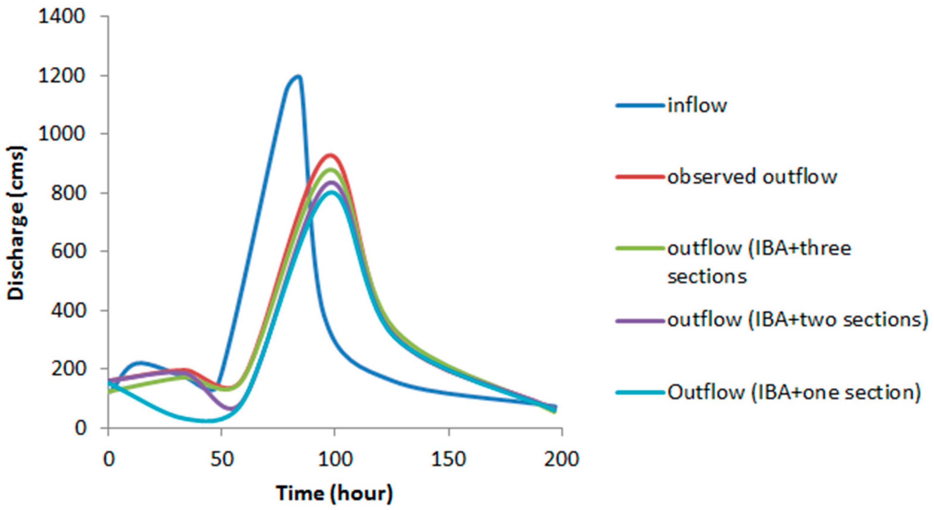
An increase in the number of reaches for evolutionary algorithms increased the accuracy of flood routing. Figure 3 shows the performance of IBA for flood routing with one, two, and three reaches, which is more consistent with observed discharges. Moreover, the computational time showed better performance for the IBA, compared to the other algorithms. For example, the computational time for the IBA based on one reach was 5s, whilst it was 7, 8, and 9s for the BA, PSO, and GA, respectively.

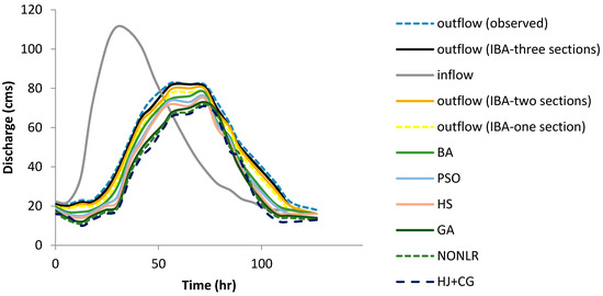
Figure 3. The simulated Hydrographs for Wilson flood using different methods.

3.3. Karahan Flood

Karahan et al. [22] routed a flood using various algorithms. This study considered the 1960 flood on the River Wye, Uk. River Wye is 69.75 km from Erwood to Belmont with consideration of lateral inflow, which was ignored in the previous studies, as shown in Table 7. In this study, the proposed model was evaluated considering the flood routing based on lateral inflow, which occurred in this Karahan flood. The data was extracted from Karahan [22].

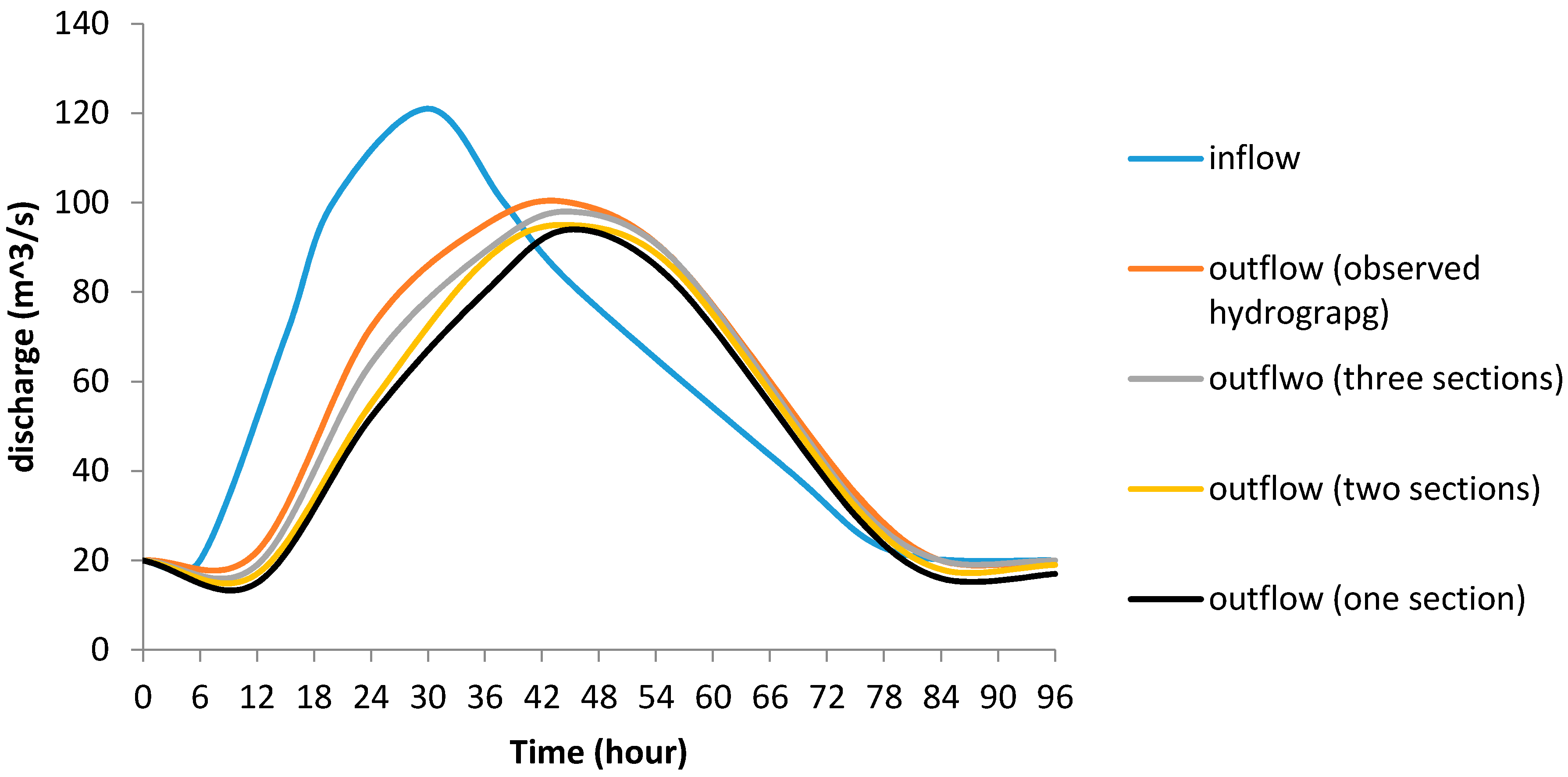
This flood was also used in the present study. The population used for IBA was 50, the maximum frequency was 5, the minimum frequency was zero, and the maximum sound loudness was 95%. In addition, the number of chromosomes for GA was 50, the probability of mutation was 0.6, and the recombination rate was 0.7. Furthermore, the number of particles used in the particle swarm algorithm was 50, the inertia coefficient was 0.7, and the personal and global learning coefficients were 2. Table 6 shows a comparison of algorithms used in flood routing in a single reach. The value of SSD for IBA was 17,120.21, which had reduced by 81%, 87%, 84%, and 10% compared with PSO, GA, HS, BA, respectively. In addition, SAD for IBA was 117, which had reduced by 83%, 88%, 94%, and 12% compared to PSO, GA, HS, and BA, respectively. The other error indices also showed a more favorable performance of IBA, compared to other algorithms. The predicted peak discharge difference with observed discharge was 0.002 cm, which was less than the other algorithms (Table 6). The time difference between predicted and observed discharge peak time for IBA was one hour, whilst this time for other algorithms was 6 hours, so IBA had a better performance. In addition, VarexQ for IBA had a larger value than other methods, which indicated a better performance. The difference of peak discharge based on IBA with observed peak was 69 cms (the closest value to the observed one), whilst it was 135 cms, 134 cms, and 70 cms for HS, PSO, and BA, respectively.

Table 6. Inflow and outflow for Karahan flood.

Time (h)	Inflow (cms)	Observed Outflow (cms)	HS [2,25]	GA	PSO	BA	Present Study IBA
0	154	102	154	132	102	102	102
6	150	140	154	152.21	154	137.89	137.24
12	219	169	152	153.44	152.1	165.78	166.12
18	182	190	181	178.11	179.4	185.43	186.11
24	182	209	191	190.45	190.9	209.01	207.12
30	192	218	185	185.1	185.4	212.32	214.33
36	165	210	187	188.21	186.9	204.45	205.24
42	150	194	179	179.45	180.20	191.32	192.12
48	128	172	162	163.11	164.10	10.45	171.25
54	168	149	141	142.11	143.70	141.44	141.38
60	260	136	154	151.12	152.8	132.22	133.56
66	471	228	198	197.11	196.3	221.14	222.21
72	717	303	264	265.21	267.3	299.12	301.12
78	1092	366	344	349.10	351.4	387.12	385.21
84	1145	456	416	423.11	431.8	451.22	453.12
90	600	615	599	600.12	617.4	610.34	611.21
96	365	830	871	872.32	881.5	826.34	827.12
102	277	969	834	835.11	836.6	899.34	900.12
108	277	665	689	690.11	696.2	667.24	665.21
114	187	519	535	534.11	549.2	522.34	520.21
120	161	444	397	400.1	416.8	455.67	453.11
126	143	321	283	287.10	305.10	314.32	316.11
132	126	208	202	203.11	221.4	212.22	210.25
138	115	176	152	155.21	164.9	177.54	170.10
144	102	148	124	131.10	131.20	151.23	145.11
150	93	125	106	108.12	110.0	127.34	119.14
156	88	114	94	106.21	96.04	116.34	112.10
162	82	106	88	88.23	89.20	107.21	105.10
168	76	97	82	81.21	82.70	92.12	93.43
174	73	89	75	76.11	76.30	91.23	88.11
180	70	81	73	73.10	73.10	82.34	80.21
186	67	76	69	69	69.80	78.12	75.10
192	63	71	66	66	66.7	72.34	69.21
198	59	66	62	62	62.40	65.21	64
SSD	-	-	37,944.14	32,944.14	31,099.52	19,122.23	17,120.21
SAD			2162	1012	695	134	117
EP			0.278	0.078	0.090	0.068	0.002
ETP			6	6	6	1	1
MARE			0.33	0.10	0.09	0.02	0.01
VarexQ			83.29	84.78	98.05	98.12	99.15

Table 7 compares IBA, BA, GA, and PSO in flood routing (Karahan flood) for single, two, and three reaches. SSD for IBA for three reaches was 16,098.21, which was 6 percent lower than for a single reach with IBA. Moreover, SAD for IBA for three reaches was 102, which had decreased by 12% compared to a single reach. Thus, IBA had an improved performance in routing with three reaches relative to single and two intervals. This was also true for the other algorithms, as shown in Table 5. Figure 4 also shows the superior performance of IBA based on three reaches. SSD using IBA for three reaches was reduced by 46%, 51%, and 5.3% compared to GA, PSO, and BA, respectively. Furthermore, SAD using IBA for three, two, and one reaches was reduced by 23–89%, compared to the other algorithms. As a result, IBA had a better performance than BA, GA, and PSO because the error indexes had the lowest value using the IBA, compared to the other algorithms. Examining the computation time showed that IBA achieved the optimal value of the objective function “under any number of multi-reach interval” faster than the other algorithms. The lowest value of the MARE index was the one associated with the IBA, on the other hand, this value decreased by 12% and 91% when using two and three reaches, respectively. Furthermore, the d index showed the IBA algorithm and simulated hydrographs using IBA had a better match with the observed hydrograph. Many studies did not consider investigate whether parameters generated by calibration could show different floods on the same river reach. In this article, this issue was considered. The optimal parameters based on IBA and three intervals for the flood event in December 1960, were used to obtain the output hydrograph for a flood on the same river on the another flood event in January 1969, based on the inflow hydrograph on January 1969, and it was considered as the first scenario. Then, the output hydrograph was extracted based on application of obtained parameters of Muskingum models for January 1969. It meant that the model was calibrated with the 1960 storm “first scenario”.

Table 7. Results of four models (i.e., IBA, BA, PSO and GA) for Karahan flood according to three different intervals.

Method	K	X	m	$\mathit{\beta }$	SSD	SAD	EP	ETP	MARE	VarexQ	Time (s)	d
	One section
IBA	0.612	0.401	1.633	0.0142	17,120.21	117	0.002	1	0.01	99.15	6	0.94
BA	0.616	0.422	1.654	0.0136	19,122.23	134	0.068	1	0.02	98.12	9	0.93
PSO	0.586	0.365	1.545	0.0138	31,099.51	695	0.090	6	0.09	98.05	10	0.90
GA	0.456	0.322	1.824	0.0137	32,944.14	1012	0.078	6	0.10	94.078	12	0.89
	Two sections
IBA	K1 = 0.672 K2 = 0.524	X1 = 0.382 X2 = 0.375	m1 = 1.723 m2 = 1.645	${\beta }_1=0.0174$ ${\beta }_2=0.0154$	17,091.20	115	0.002	1	0.01	99.25	8	0.93
BA	K1 = 0.652 K2 = 0.521	X1 = 0.352 X2 = 0.355	m1 = 1.623 m2 = 1.642	${\beta }_1=0.0214$ ${\beta }_2=0.0124$	17,114.25	122	0.058	1	0.01	99.15	11	0.90
PSO	K1 = 0.112 K2 = 0.110	X1 = 0.289 X2 = 0.284	m1 = 1.623 m2 = 1.545	${\beta }_2=0.0064$ ${\beta }_2=0.0039$	30,235.45	687	0.088	6	0.08	98.12	14	0.89
GA	K1 = 0.78 K2 = 0.689	X1 = 0.244 X2 = 0.232	m1 = 1.611 m2 = 1.811	${\beta }_1=0.0027$ ${\beta }_2=0.0029$	31,231.23	1009	0.068	6	0.10	94.79	16	0.88
	Three sections
IBA	K1 = 0.692 K2 = 0.690 K3 = 0.612	X1 = 0.392 X2 = 0.391 X3 = 0.394	m1 = 1.112 m2 = 1.114 m3 = 1.116	${\beta }_1=0.0178$ ${\beta }_2=0.0162$ ${\beta }_3=0.0144$	16,098.21	102	0.002	1	0.008	99.56	10	0.91
BA	K1 = 0.694 K2 = 0.696 K3 = 0.622	X1 = 0.394 X2 = 0.399 X3 = 0.394	m1 = 1.115 m2 = 1.117 m3 = 1.116	${\beta }_1=0.0074$ ${\beta }_2=0.0124$ ${\beta }_3=0.0134$	16,999.21	108	0.0038	1	0.009	99.54	15	0.86
PSO	K1 = 0.237 K2 = 0.312 K3 = 0.321	X1 = 0.298 X2 = 0.321 X3 = 0.312	m1 = 1.311 m2 = 1.411 m3 = 1.512	${\beta }_1=0.0044$ ${\beta }_1=0.0029$ $\beta 3=0.0020$	30,230.21	667	0.081	6	0.06	99.11	17	0.84
GA	K1 = 0.900 K2 = 0.878 K3 = 0.815	X1 = 0.296 X2 = 0.294 X3 = 0.224	m1 = 1.655 m2 = 1.652 m3 = 1.651	${\beta }_1=0.0014$ ${\beta }_2=0.0012$ ${\beta }_3=0.0010$	30,298.11	987	0.057	6	0.09	96.12	19	0.82

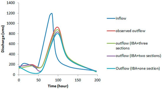
Figure 4. Simulated hydrograph for Karahan flood.

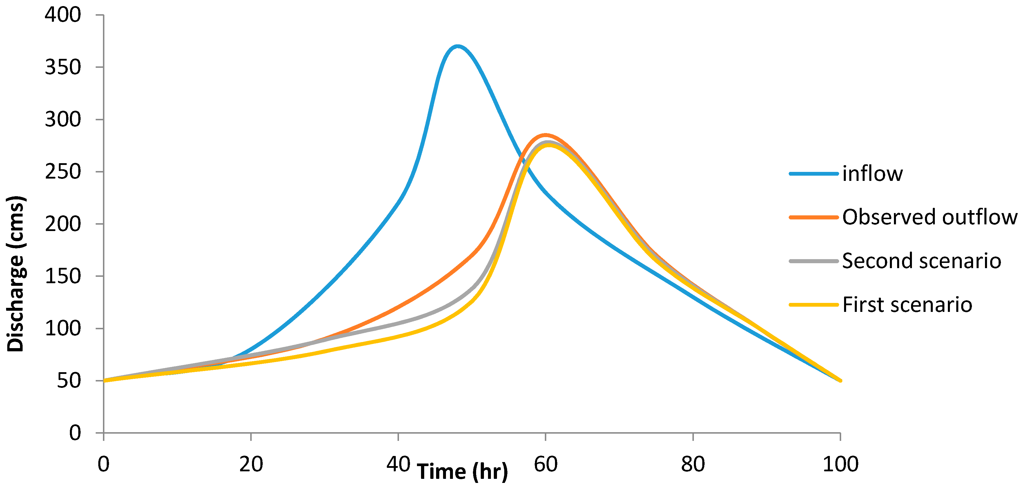
The value of SSD for the first scenario was 878 and the peak value was 280 cms, whilst the observed peak value was 285 and there was a small difference between the observed and the simulated peak value (Figure 5). The SSD for the second scenario was 869 and the peak value was 282 cms. Although, the second scenario acted better than the first scenario, the results for the first scenario were acceptable. The results were so similar because of the accurate sensitivity analysis considered for the Muskingum model for the objective function and different parameters, such as in pervious sections. Although the proposed model structure successfully predicted the flood routing, further research could consider different Muskingum models based on more parameters to investigate the performance of IBA. In addition, application of these models helps the hydraulic designers to have the accurate value for the peak discharge and the flood characteristics, to be able to optimally design the target structure.

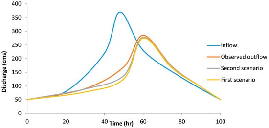
Figure 5. The first and second scenario for calibration of model.

3.4. Chindwin River

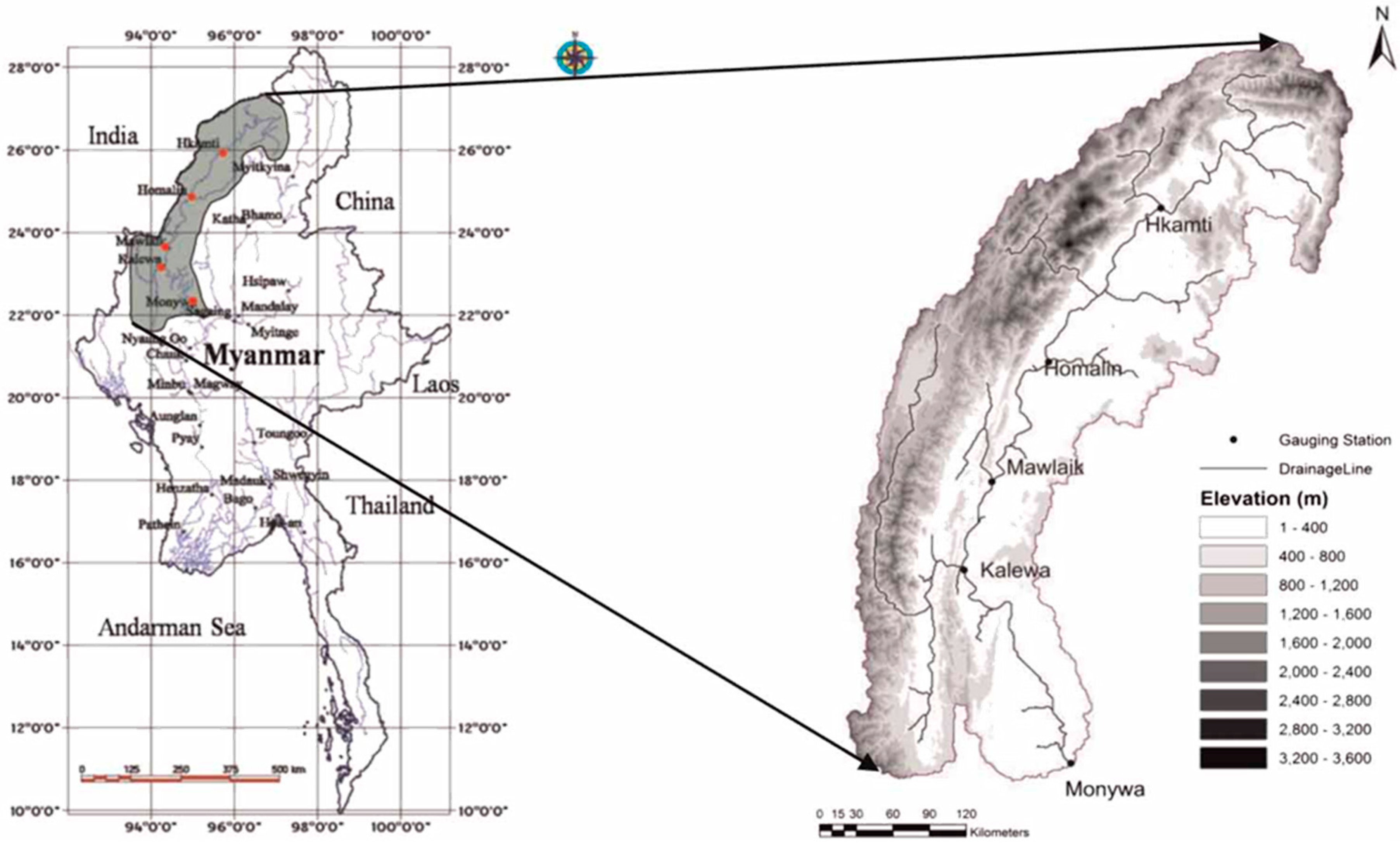
One of the most important Myanmar Rivers is the Chindwin River, shown in Figure 6. This river, over the past twenty years, has experienced many floods. Due to severe flood conditions, the construction of hydraulic structures and living conditions in the downstream areas are difficult and there is high lateral inflow for this basin. Therefore, it is important to predict river flood conditions. The length of the river is 114 km and the surface of the basin is 7485 km². A historical flood considered in this study occurred in July 2004, and the Mawliak Station recording the flood is shown in Figure 5. Table 8 shows a comparison of different methods for the first flood with flood routing using a single reach. Comparing IBA, BA, GA, and PSO based on routing with a single reach, SSD for IBA relative to GA, BA, and PSO was reduced by 32%, 11%, and 42%, respectively. For routing with two reaches, SSD for IBA was reduced by 33%, 34%, and 12% compared to PSO, GA, and BA, respectively. For three reaches, SSD for IBA was reduced by 44%, 50%, and 37% compared to PSO, GA and BA, respectively. The SAD index for the three routings indicated the superiority of IBA. Comparison of routing with three, two, and one reaches indicated that three reaches improved routing. SSD in relation to routing with two and one reaches had reduced by 39% and 20%, respectively. ETp showed that there was no time lag in forecasting of peak flow by different algorithms. VarexQ showed that three-reach routing was better than two and one reach routings. Additionally, MARE for IBA-based routing had reduced by 64% and 62%, relative to one and two reach routing, respectively. Figure 7 shows that the three reach flood routing was superior to that based on two and single reaches. The results indicated that the IBA has the less computational time compared to the other algorithms, as shown in Table 6. In addition, considering the attained value of the d index, it was obvious that IBA had the best performance compared to the other algorithms.

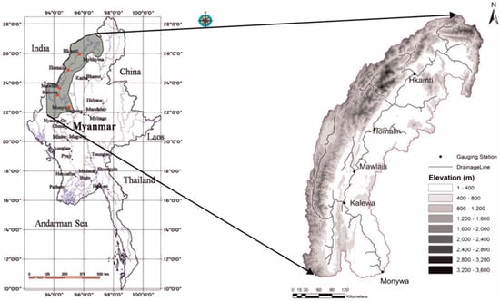
Figure 6. The location of the River in Myanmar.

Table 8. The computed error indexes for Myanmar River.

Method	K	X	m	$\mathit{\beta }$	SSD	SAD	EP	ETP	MARE	VarexQ	Time (s)	d
One section
IBA	0.411	0.301	1.611	0.0344	8.24	2.12	0.002	0	0.015	99.22	7	0.93
BA	0.410	0.304	1.612	0.321	9.22	3.14	0.004	0	0.017	99.16	9	0.92
PSO	0.386	0.255	1.545	0.0265	12.22	3.24	0.078	0	0.095	98.15	10	0.89
GA	0.256	0.312	1.524	0.0222	14.25	4.25	0.089	0	0.102	94.78	11	0.87
Two sections
IBA	K1 = 0.472 K2 = 0.424	X1 = 0.392 X2 = 0.365	m1 = 1.721 m2 = 1.635	${\beta }_1=0.0212$ ${\beta }_2=0.0139$	7.99	2.10	0.002	0	0.014	99.25	10	0.91
BA	K1 = 0.479 K2 = 0.428	X1 = 0.394 X2 = 0.368	m1 = 1.821 m2 = 1.433	${\beta }_1=0.0210$ ${\beta }_2=0.0131$	9.11	2.89	0.003	0	0.016	99.18	12	0.90
PSO	K1 = 0.102 K2 = 0.110	X1 = 0.279 X2 = 0.224	m1 = 1.622 m2 = 1.542	${\beta }_1=0.0197$ ${\beta }_1=0.0190$	11.95	3.09	0.088	0	0.088	98.22	14	0.89
GA	K1 = 0.78 K2 = 0.789	X1 = 0.244 X2 = 0.212	m1 = 1.610 m2 = 1.611	${\beta }_1=0.0196$ ${\beta }_2=0.0188$	12.24	4.55	0.068	0	0.100	94.89	16	0.87
Three sections
IBA	K1 = 0.492 K2 = 0.491 K3 = 0.512	X1 = 0.292 X2 = 0.261 X3 = 0.294	m1 = 1.110 m2 = 1.112 m3 = 1.114	${\beta }_1=0.0342$ ${\beta }_2=0.0288$ ${\beta }_3=0.0488$	5.12	1.98	0.002	0	0.005	99.56	18	0.91
BA	K1 = 0.412 K2 = 0.471 K3 = 0.514	X1 = 0.291 X2 = 0.254 X3 = 0.292	m1 = 1.112 m2 = 1.114 m3 = 1.116	${\beta }_1=0.0342$ ${\beta }_2=0.0148$ ${\beta }_3=0.0138$	8.11	2.10	0.005	0	0.003	99.41	20	0.90
PSO	K1 = 0.236 K2 = 0.311 K3 = 0.319	X1 = 0.295 X2 = 0.320 X3 = 0.310	m1 = 0.211 m2 = 0.221 m3 = 0.212	${\beta }_1=0.0221$ ${\beta }_2=0.0212$ ${\beta }_2=0.0217$	9.27	2.12	0.081	0	0.0612	99.31	22	0.87
GA	K1 = 0.910 K2 = 0.876 K3 = 0.815	X1 = 0.396 X2 = 0.396 X3 = 0.324	m1 = 1.655 m2 = 1.652 m3 = 1.651	${\beta }_1=0.0251$ ${\beta }_2=0.0218$ ${\beta }_2=0.0217$	10.12	3.25	0.057	0	0.090	96.18	24	0.85

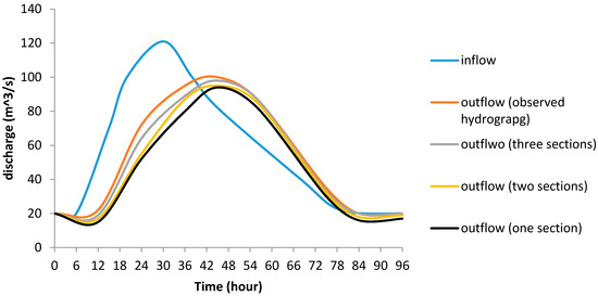
Figure 7. Simulated hydrograph for Myanmar River using IBA.

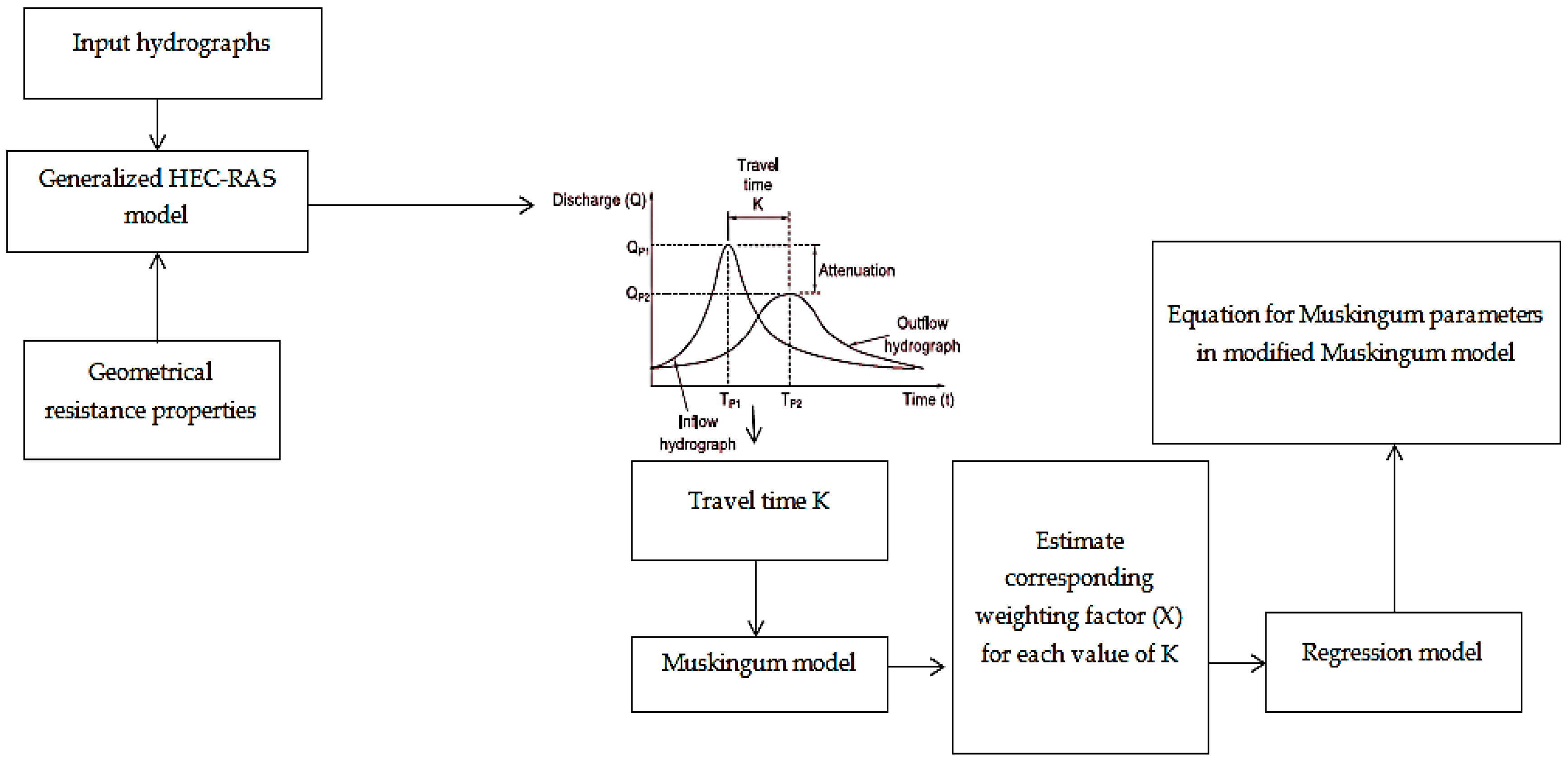
To enhance further, the used structure of the proposed Muskingum model coupled with IBA showed the highest abilities, for studying the flood plain with back water. Furthermore, such enhancement for the Muskingum model could be successfully applied as an easy and inexpensive method for computing the time and shape, for an overbank flood, when there is back water and inertia influences along a river channel. In fact, with the new nature-inspired optimization algorithms, the traditional Muskingum method could be integrated with the hydrodynamic software packages, such as HEC-RAS model. The development procedure could be carried out by utilizing HEC-RAS software as the model input for hydrographs and geometric characteristic, to estimate the travel times and attenuations peak, whilst the weighted coefficient (X) value could be achieved based on the optimization model and Muskingum model, as shown in Figure 8. As a result, the proposed model in this research showed the potential to be suitable and appropriate for studying and analyzing flood propagation and flood mapping.

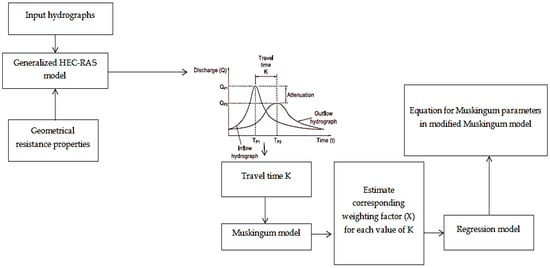
Figure 8. Advanced Muskingum model for flood plain with complex boundary condition.

4. Conclusions

The present study investigated the potential of utilizing a three-parameter Muskingum model coupled with Improved Bat Algorithm (IBA) to accurately predict flood routing. Three different case studies have been used in this study, to evaluate the performance of the proposed model. These three case studies were the Wilson flood, Karahan flood, and Myanmar River. Seven different performance indices were used to examine and compare the performance of the proposed model over other algorithms. In addition, discretization of the river stream was considered to improve model accuracy. The results showed that IBA outperformed all other algorithms and was able to reduce the SSD by percentages ranging between 20% and 84%, compared with the other algorithms. In addition, the achieved results using the IBA could predict the peak discharge accurately, with a value very close to the observed one. Under the Karahan flood, IBA considerably achieved the minimum level of error indices for a single reach, compared to other algorithms. Finally, IBA in flood routing with three intervals had a better performance than with single and two reaches. The division of the river into different reaches increased the accuracy of flood routing. The performance of IBA for the river in Myanmar, also showed that the simulated hydrograph with three reaches was more accurate. For example, the computational time for the IBA based on three intervals was 2, 4, and 6 s less than, BA, PSO, and GA, respectively. Furthermore, the EP for the IBA was 33%, 96%, and 97% less than BA, PSO, and GA, respectively. As a result, the proposed Muskingum model coupled with the IBA, could be considered as a strong alternative method for predicting flood routing characteristics.

References

- Barati, R.; Badfar, M.; Azizyan, G.; Akbari, G.H. Discussion of “Parameter Estimation of Extended Nonlinear Muskingum Models with the Weed Optimization Algorithm” by Farzan Hamedi, Omid Bozorg-Haddad, Maryam Pazoki, Hamid-Reza Asgari, Mehran Parsa, and hugo a. Loáiciga. J. Irrig. Drain. Eng. 2018, 144, 7017021. [Google Scholar] [CrossRef]
- Hamedi, F.; Bozorg-Haddad, O.; Pazoki, M.; Asgari, H.R.; Parsa, M.; Loáiciga, H.A. Parameter estimation of extended nonlinear muskingum models with the weed optimization algorithm. J. Irrig. Drain. Eng. 2016, 142, 4016059. [Google Scholar] [CrossRef]
- Zhang, S.; Kang, L.; Conservation, B.Z. Parameter estimation of nonlinear muskingum model with variable exponent using adaptive genetic algorithm. In Environmental Conservation, Clean Water, Air & Soil (CleanWAS); IWA Publishing: London, UK, 2017; pp. 231–234. [Google Scholar]
- Bradbrook, K.F.; Lane, S.N.; Waller, S.G.; Bates, P.D. Two dimensional diffusion wave modelling of flood inundation using a simplified channel representation. Int. J. River Basin Manag. 2004, 2, 211–223. [Google Scholar] [CrossRef]
- Neal, J.; Villanueva, I.; Wright, N.; Willis, T.; Fewtrell, T.; Bates, P. How much physical complexity is needed to model flood inundation? Hydrol. Process. 2012, 26, 2264–2282. [Google Scholar] [CrossRef]
- Hunter, N.M.; Bates, P.D.; Neelz, S.; Pender, G.; Villanueva, I.; Wright, N.G.; Liang, D.; Falconer, R.A.; Lin, B.; Waller, S.; et al. Benchmarking 2D hydraulic models for urban flooding simulations. Proc. Inst. Civ. Eng. Water Manag. 2008, 161, 13–30. [Google Scholar] [CrossRef]
- Dottori, F.; Todini, E. Testing a simple 2D hydraulic model in an urban flood experiment. Hydrol. Process. 2013, 27, 1301–1320. [Google Scholar] [CrossRef]
- Kim, B.; Sanders, B.F.; Schubert, J.E.; Famiglietti, J.S. Mesh type tradeoffs in 2D hydrodynamic modeling of flooding with a godunov-based flow solver. Adv. Water Resour. 2014, 68, 42–61. [Google Scholar] [CrossRef]
- Prestininzi, P. Suitability of the diffusive model for dam break simulation: Application to a cadam experiment. J. Hydrol. 2008, 361, 172–185. [Google Scholar] [CrossRef]
- Aricò, C.; Sinagra, M.; Begnudelli, L.; Tucciarelli, T. MAST-2D diffusive model for flood prediction on domains with triangular Delaunay unstructured meshes. Adv. Water Resour. 2011, 34, 1427–1449. [Google Scholar] [CrossRef]
- Schubert, J.E.; Sanders, B.F.; Smith, M.J.; Wright, N.G. Unstructured mesh generation and landcover-based resistance for hydrodynamic modeling of urban flooding. Adv. Water Resour. 2008, 31, 1603–1621. [Google Scholar] [CrossRef]
- Bates, P.D.; Horritt, M.S.; Fewtrell, T.J. A simple inertial formulation of the shallow water equations for efficient two-dimensional flood inundation modelling. J. Hydrol. 2010, 387, 33–45. [Google Scholar] [CrossRef]
- Costabile, P.; Costanzo, C.; Macchione, F. Performances and limitations of the diffusive approximation of the 2-D shallow water equations for flood simulation in urban and rural areas. Appl. Numer. Math. 2017, 116, 141–156. [Google Scholar] [CrossRef]
- Fassoni-Andrade, A.C.; Fan, F.M.; Collischonn, W.; Fassoni, A.C.; Paiva, R.C. Comparison of numerical schemes of river flood routing with an inertial approximation of the Saint Venant equations. RBRH 2018, 23, e10. [Google Scholar] [CrossRef]
- Singh, V.P.; Aravamuthan, V. Errors of kinematic-wave and diffusion-wave approximations for steady-state overland flows. Catena 1996, 27, 209–227. [Google Scholar] [CrossRef]
- Costabile, P.; Macchione, F.; Natale, L.; Petaccia, G. Flood mapping using LIDAR DEM. Limitations of the 1-D modeling highlighted by the 2-D approach. Nat. Hazards 2015, 77, 181–204. [Google Scholar] [CrossRef]
- Chatila, J.G. Muskingum Method, EXTRAN and ONE-D for routing unsteady flows in open channels. Can Water Resour. J. 2003, 28, 481–498. [Google Scholar] [CrossRef]
- O’Sullivan, J.J.; Ahilan, S.; Bruen, M. A modified Muskingum routing approach for floodplain flows: Theory and practice. J. Hydrol. 2012, 470, 239–254. [Google Scholar]
- Yoo, C.; Lee, J.; Lee, M. Parameter Estimation of the Muskingum Channel Flood-Routing Model in Ungauged Channel Reaches. J. Hydrol. Eng. 2017, 22, 5017005. [Google Scholar] [CrossRef]
- Geem, Z.W. Parameter Estimation of the Nonlinear Muskingum Model Using Parameter-Setting-Free Harmony Search. J. Hydrol. Eng. 2011, 16, 684–688. [Google Scholar] [CrossRef]
- Barati, R. Parameter estimation of nonlinear Muskingum models using Nelder-Mead simplex algorithm. J. Hydrol. Eng. 2011, 16, 946–954. [Google Scholar] [CrossRef]
- Karahan, H.; Gurarslan, G.; Geem, Z.W. Parameter estimation of the nonlinear Muskingum flood-routing model using a hybrid harmony search algorithm. J. Hydrol. Eng. 2013, 18, 352–360. [Google Scholar] [CrossRef]
- Orouji, H.; Bozorg Haddad, O.; Fallah-Mehdipour, E.; Mariño, M.A. Estimation of Muskingum parameter by meta-heuristic algorithms. Proc. Inst. Civ. Eng. Water Manag. 2013, 166, 315–324. [Google Scholar] [CrossRef]
- Easa, S.M. New and improved four-parameter non-linear Muskingum model. Proc. Inst. Civ. Eng. Water Manag. 2014, 167, 288–298. [Google Scholar] [CrossRef]
- Talatahari, S.; Sheikholeslami, R.; Farahmand Azar, B.; Daneshpajouh, H. Optimal Parameter Estimation for Muskingum Model Using a CSS-PSO Method. Adv. Mech. Eng. 2013, 5, 480954. [Google Scholar] [CrossRef]
- Ouyang, A.; Li, K.; Truong, T.K.; Sallam, A.; Sha, E.H.-M. Hybrid particle swarm optimization for parameter estimation of Muskingum model. Neural Comput. Appl. 2014, 25, 1785–1799. [Google Scholar] [CrossRef]
- Geem, Z.W. Issues in optimal parameter estimation for the nonlinear Muskingum flood routing model. Eng. Optim. 2014, 46, 328–339. [Google Scholar] [CrossRef]
- Haddad, O.B.; Hamedi, F.; Fallah-Mehdipour, E.; Orouji, H.; Mariño, M.A. Application of a hybrid optimization method in Muskingum parameter estimation. J. Irrig. Drain. Eng. 2015, 141, 4015026. [Google Scholar] [CrossRef]
- Niazkar, M.; Afzali, S.H. Assessment of modified honey bee mating optimization for parameter estimation of nonlinear Muskingum models. J. Hydrol. Eng. 2015, 20, 4014055. [Google Scholar] [CrossRef]
- Moghaddam, A.; Behmanesh, J.; Farsijani, A. Parameters estimation for the new four-parameter nonlinear muskingum model using the particle swarm optimization. Water Resour. Manag. 2016, 30, 2143–2160. [Google Scholar] [CrossRef]
- Kang, L.; Zhang, S. Application of the elitist-mutated PSO and an improved GSA to estimate parameters of linear and nonlinear Muskingum flood routing models. PLoS ONE 2016, 11, e0147338. [Google Scholar] [CrossRef] [PubMed]
- Lee, E.; Lee, H.; Kim, J. Development and Application of Advanced Muskingum Flood Routing Model Considering Continuous Flow. Water 2018, 10, 760. [Google Scholar] [CrossRef]
- Wang, L.; Lapin, S.; Wu, J.Q.; Elliot, W.J.; Fiedler, F.R. Accuracy of the Muskingum-Cunge method for constant-parameter diffusion-wave channel routing with lateral inflow. arXiv, 2018; arXiv:1802.04429. [Google Scholar]
- Jamil, M.; Zepernick, H.J.; Yang, X.S. Multimodal Function Optimization Using an Improved Bat Algorithm in Noise-Free and Noisy Environments. In Nature-Inspired Computing and Optimization; Patnaik, S., Yang, X.-S., Nakamatsu, K., Eds.; Modeling and Optimization in Science and Technologies; Springer International Publishing: Basel, Switzerland, 2017; Volume 10, pp. 29–49. [Google Scholar]
- Bozorg-Haddad, O.; Karimirad, I.; Seifollahi-Aghmiuni, S.; Loáiciga, H.A. Development and application of the bat algorithm for optimizing the operation of reservoir systems. J. Water Resour. Plan. Manag. 2015, 141, 4014097. [Google Scholar] [CrossRef]
- Ahmadianfar, I.; Adib, A.; Salarijazi, M. Optimizing multireservoir operation: hybrid of bat algorithm and differential evolution. J. Water Resour. Plan. Manag. 2016, 142, 5015010. [Google Scholar] [CrossRef]
- Cai, X.; Wang, H.; Cui, Z.; Cai, J.; Xue, Y.; Wang, L. Bat algorithm with triangle-flipping strategy for numerical optimization. Int. J. Mach. Learn. Cybern. 2018, 9, 199–215. [Google Scholar] [CrossRef]
- Chakri, A.; Khelif, R.; Benouaret, M.; Yang, X.S. New directional bat algorithm for continuous optimization problems. Expert Syst. Appl. 2017, 69, 159–175. [Google Scholar] [CrossRef]
- Ehteram, M.; Allawi, M.; Karami, H.; Mousavi, S. Optimization of Chain-Reservoirs’ Operation with a New Approach in Artificial Intelligence. Water Resour. 2017, 31, 2085–2104. [Google Scholar] [CrossRef]
- Allawi, M.F.; Jaafar, O.; Ehteram, M.; Mohamad Hamzah, F.; El-Shafie, A. Synchronizing Artificial Intelligence Models for Operating the Dam and Reservoir System. Water Resour. Manag. 2018, 32, 3373–3389. [Google Scholar] [CrossRef]
- Allawi, M.F.; Jaafar, O.; Mohamad Hamzah, F.; Abdullah, S.M.S.; El-shafie, A. Review on applications of artificial intelligence methods for dam and reservoir-hydro-environment models. Environ. Sci. Pollut. Res. 2018, 25, 13446–13469. [Google Scholar] [CrossRef] [PubMed]
- Allawi, M.F.; Jaafar, O.; Mohamad Hamzah, F.; Ehteram, M.; Hossain, M.S.; El-Shafie, A. Operating a reservoir system based on the shark machine learning algorithm. Environ. Earth Sci. 2018, 77, 366. [Google Scholar] [CrossRef]
- El-shafie, A.; Mukhlisin, M.; Najah, A.A.; Taha, M.R. Performance of artificial neural network and regression techniques for rainfall-runoff prediction. Int. J. Phys. Sci. 2011, 6, 1997–2003. [Google Scholar]
- Wilson, E.M. Engineering Hydrology; Palgrave: London, UK, 1990; pp. 1–49. [Google Scholar]
- Legates, D.R.; McCabe, G.J. Evaluating the use of “goodness-of-fit” Measures in hydrologic and hydroclimatic model validation. Water Resour. Res. 1999, 35, 233–241. [Google Scholar] [CrossRef]
- Ehteram, M.; Binti Othman, F.; Mundher Yaseen, Z.; Abdulmohsin Afan, H.; Falah Allawi, M.; Najah Ahmed, A.; Shahid, S.; Singh, V.P.; El-Shafie, A. Improving the Muskingum flood routing method using a hybrid of particle swarm optimization and bat algorithm. Water 2018, 10, 807. [Google Scholar] [CrossRef]
© 2018 by the authors. Licensee MDPI, Basel, Switzerland. This article is an open access article distributed under the terms and conditions of the Creative Commons Attribution (CC BY) license (http://creativecommons.org/licenses/by/4.0/).