1. Introduction
A dam is continuously in harmonic motion due to environmental factors, such as wind, water waves, floods, and earthquakes. In addition, the operation of a dam powerhouse produces harmonic motion that affects dam stability. Dams can be classified according to different criteria. Based on materials used in construction, dams are categorized into masonry, concrete, and embanked dams (earth and rock-fill). In addition to the main dam structure, dam appurtenances such as spillways, conduits, and powerhouses are necessary for the dam. According to Bosshard, more than 80% of the total constructed dams in China are embankment dams [
1]. In Québec, Canada, embankment dams account for about 73% of the total dams in this territory. Most of the past dam failures and incidents happened at sites with embankment dams. Thus, more studies are required to increase the safety of embankment dams. A revolution in technology occurred in the late 19th century when an electric generator was driven by a hydro-turbine on Fox River in Wisconsin, USA [
2]. This invention gave birth to hydropower technology.
1.1. Vibrations of Turbines and Powerhouses
The powerhouse represents one of the main parts of the dam used to generate hydroelectric power at low cost. The detection of the hydraulic characteristics in reaction turbines is the key to determining the effect of turbine operation on the dam body [
3]. Based on a literature review, numerous investigations have been conducted utilizing those tools to simulate the flow behavior in the draft tube of turbine sand to inspect the critical conditions, such as the vortex rope and vibration [
4,
5]. Researchers have studied pressure pulsation in Francis hydraulic turbine units and discussed the cavitation phenomenon problem [
6,
7].
Jošt and Lipej built a three-dimensional (3D) numerical model for a Francis turbine unit to predict the vortex rope in the draft tube based on numerical flow analyses by performing two analyses, both with and without cavitation effects [
8]. Another study reported a numerical analysis of the cavitation turbulent flow in a Francis turbine under partial load operation using the
k–ω shear stress transport turbulence model in the Reynolds-averaged Navier-Stokes equations [
9]. Qian et al. simulated 3D multiphase flows in a Francis turbine to calculate pressure pulsation in the spiral casing, draft tube, runner front, and guide vanes using fast Fourier transform [
10]. Anup et al. investigated the hydrodynamic effects of pressure fluctuation in the draft [
11]. The cause of rotor-stator interaction simulation under partial load operation, using analyzing 3D transient state turbulence flow simulation in a Francis tube, was investigated. The 3D Navier-Stokes computational fluid dynamics (CFD) solver ANSYS-CFX was used to analyze the flow through a vertical Francis turbine with different loads in situ. Most lately, Luna-Ramírez et al. calculated the pressure on the blades of a 200 MW Francis hydraulic turbine to locate the failure on the blade surface based on CFD [
12]. There are also several other studies analyzing the Francis turbine using the advantages of computational features [
13,
14,
15,
16].
1.2. Powerhouse Vibration Analysis
Caishui studied the pressure distribution in the flow pattern within a powerhouse using the fluid dynamics method [
17]. Caishui developed a mathematical model for a specific powerhouse station to find the velocity distribution and the pressure pattern distribution under three operating conditions (one-unit load, two-unit load, and full load rejection). The results of the study showed a good flow pattern at the inlet with steady water level fluctuation. Wel and Zhang created a 3D numerical model for a powerhouse body using ANSYS software to determine the stress and strain in the powerhouse body, and pressure, acceleration, and the frequency within the powerhouse [
18]. ANSYS software is an American engineering solution based in Canonsburg, Pennsylvania. They concluded that most vibration was generated because of the static and dynamic disturbance of the hydraulic turbine blades.
1.3. Vibration Effect on Dam Body
Fenves and Chopra simplified the analysis procedure of the fundamental vibration mode response of concrete gravity dam systems for two cases: (1) dams with reservoirs of impounded water supported by a rigid foundation rock, and (2) dams with empty reservoirs supported by a flexible foundation rock [
19]. In 1992, Gazetas and Dakoulas analyzed the vibration effect on a rock-filled dam depending on the diagrams presented by the effect of vibration, represented by the acceleration, displacement, shear strain, and seismic coefficients with time [
20]. The authors discussed changes in these parameters with the change in depth, starting from the crest of the dam. Finally, a dimensionless graph was used in primary engineering designs to determine the peaks of the parameters. Bouaanani et al. presented a numerical technique based on the procedure derived by Fenves and Chopra to calculate the earthquake influence that includes the hydrodynamic pressure on the rigid gravity dams, by suggesting closed-form formulas used to solve fluid–dam interaction problem [
21]. The dam-reservoir interaction effect is represented by one of the following three assumptions:
- (1)
The physical properties of the water that represents the mass of the reservoir added to the dam are defined.
- (2)
The dam-reservoir interaction is described using the Eulerian approach introduced by Bouaanani and Paultre. The variables used are the displacements in the dam, as well as the velocity and pressure potential in the water [
22].
- (3)
The dam-reservoir interaction is represented by the Lagrangian approach. The dam-reservoir behavior is expressed in terms of displacement and functions, with some constraints suggested excluding the zero-energy mode [
23,
24,
25].
Considering the complexity of the dam-reservoir-foundation geometry, most of the recent studies used two-dimensional (2D) numerical models to analyze the seismic effect on the dynamic behavior of concrete dams [
26,
27,
28] and embanked dams [
29,
30]. Most of these studies depended on the FE method concept.
Anastasiadis et al. created a 2D model for a high rock-filled dam. In this study, a model analysis method was performed depending on the mode shapes evaluated for the symmetric part of the dam body [
31]. The study depended on a special computer program MAP-76. Subsequently, with the analysis of Pine flat, the dam was considered a numerical model. This technique was applied to the dam body and the outcomes were compared with results related to direct methods of analysis.
With software developments and computer speed improvement, many researchers have analyzed the seismic effect to understand their dynamic behavior by using realistic 3D FE models instead of 2D models to represent dams [
32]. Hariri-Ardebili and Mirzabozorg studied the effect of four water levels coupled with a seismic effect on the dynamic behavior of arch dams [
33]. In another attempt, Hariri-Ardebili and Seyed-Kolbadi developed 3D FE models to represent three types of concrete dams (gravity, buttress, and arch dams). These two studies clearly defined the 3D boundary conditions for the dam-reservoir foundation interaction system [
34].
Dakoulas studied the longitudinal vibration on concrete-faced rockfill dams that cause compressive stress with a joint opening in the concrete slab panels [
32]. A 3D hyperbolic model for the rockfill was used to determine the behavior of the dams subjected to longitudinal and vertical vibrations. The analysis considered the flexibility of the rocks and possible dynamic settlements of the rockfill. The dynamic settlements effect was examined, and comparisons were made to the response from upstream to downstream and combined vibrations.
Some researchers estimated the dynamic behavior of concrete dams or rockfill dams and verified their results by comparing 3D and 2D models [
35,
36]. Other researchers compared the model results with in situ dynamic test data. However, comparing 2D and 3D models is not considered a valid strategy to verify the results because both models are prepared by the researcher. In addition, 2D models represent only one part of the dam and cannot represent irregular dams.
A dam is presented to create the head difference between the headrace (the water surface elevation upstream of the dam) and the tailrace (the water surface elevation downstream of the dam). The penstock is comprised of pipes or tunnels that direct flow to the turbine system. The hydro-turbine itself is a mechanical device whose rotation is driven by the extraction of energy from the flow. The electric generator converts mechanical energy into electrical energy and its rotation is driven by a shaft attached directly to the rotating hydro-turbine. Finally, the draft tube is a diffuser that collects the flow after it exits the turbine and deposits it on the lower side of the dam. The hydro-turbine is categorized into impulse turbines (Pelton type) and reaction turbines (Francis and Kaplan types). Based on head available between upstream and downstream of the dams, most turbines used at the powerhouse are reaction turbines. Turbine operation is a source of vibration that affects the dam and powerhouse stability.
The seismic effect on dam bodies was studied by civil engineering researchers in order to assess their dynamic behavior. Many researchers [
26,
37,
38] developed 2D numerical models for simulation of dynamic behavior of dam bodies. Other researchers [
39,
40] developed 3D numerical models that are more capable and accurate than the 2D models. The vibrational effect produced by the hydraulic turbines was studied by mechanical engineering researchers to assess their hydraulic performance due to powerhouse operation. Mechanical researchers [
3,
8,
10,
11,
12,
13,
14,
15,
16,
17,
41,
42,
43,
44,
45] focused on modeling and analysis of pressure distribution on the turbine draft tube. There is no comprehensive study connecting the vibration effect on the dam body, including the powerhouse and the vibration effect generated by operating the turbines inside the powerhouse.
1.4. Research Objectives
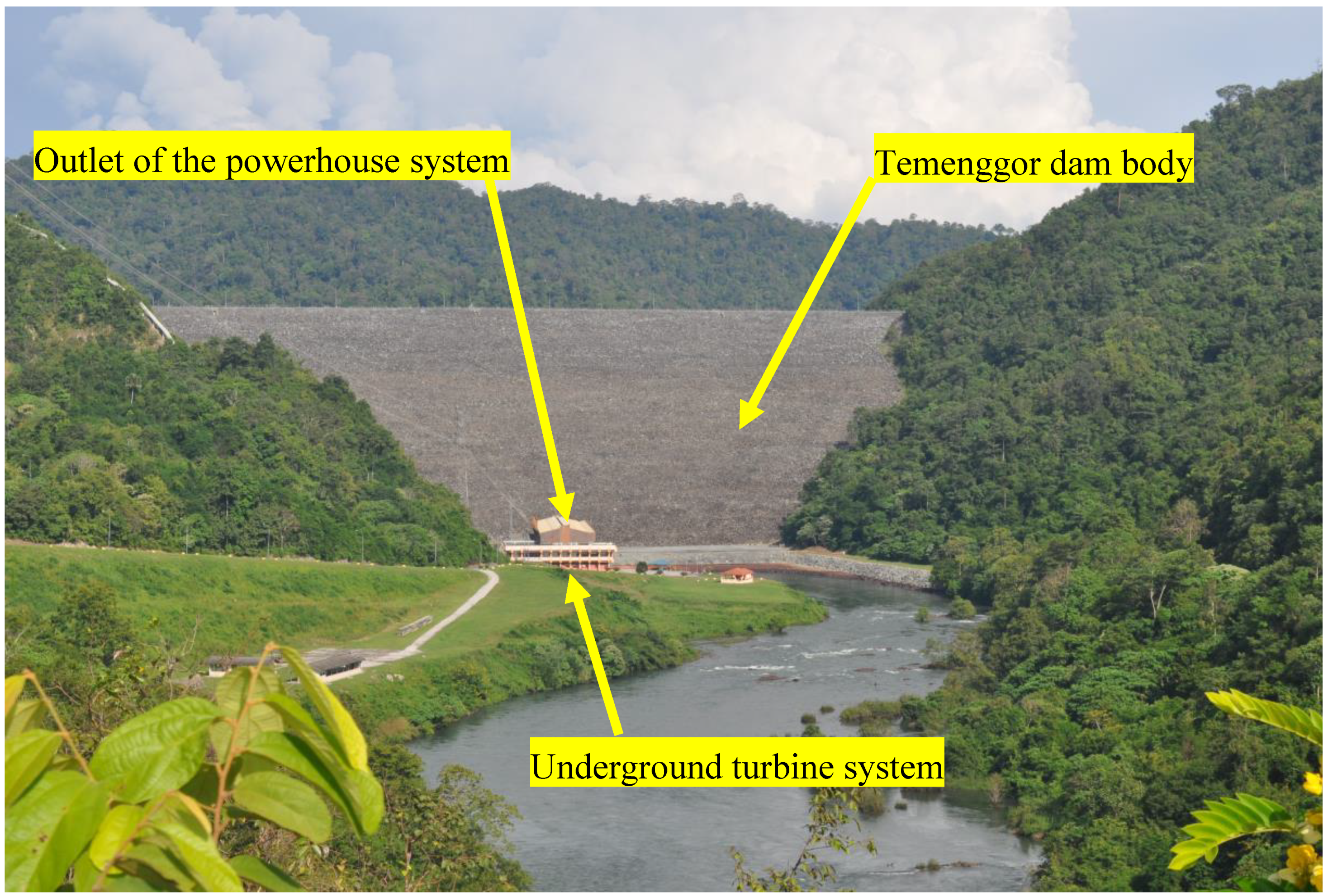
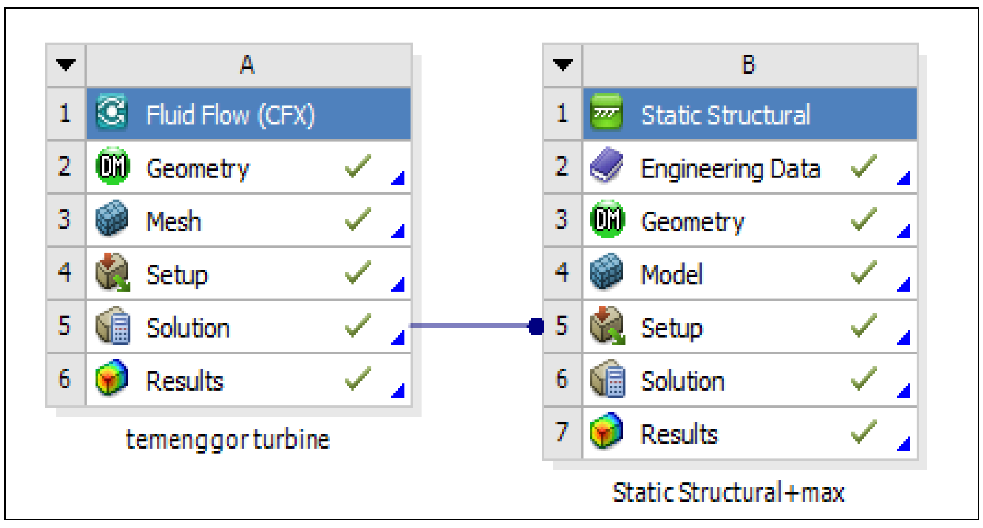
This study conducts 3D numerical modeling based on the finite element (FE) technique to assess the dynamic behavior of selected embankment dams. The hydraulic performance of the reaction turbines in the powerhouses of the selected embankment dam is assessed using 3D numerical modeling based on the finite volume technique. In the first part of this study, one reaction Francis turbine from Temenggor powerhouse is selected as a case study. ANSYS-CFX is used to develop a 3D numerical model of the turbine unit. The turbine model is run under a real head and discharge data obtained from a site visit are used to find the hydraulic performance of the turbine units.
In the second part of this study, a 3D FE numerical dam model is developed to calculate the principal stress of the dam-reservoir-foundation system with the change in water levels from the maximum drawdown to the flood level. The hydrostatic pressure and gravity are defined according to the water level considering the foundation depth (127 m) and the dam-reservoir-foundation interaction. The soil physical properties of the dam-foundation are estimated from engineering reports and water physical properties are defined. The results are obtained from the integration of 3D numerical finite element dam models with 3D numerical finite volume turbine models. The results cover all the possibilities that may arise from the operation of the powerhouses, including maximum and minimum water levels for the case of full inlet gates openings. The results of the 3D dam models include the principal stress distributions in both dams and powerhouses. The results of the 3D dam model outline an operating program for running the turbine units that minimizes the stresses on the dam and powerhouse bodies to increase the project life.
4. Hydraulic Analysis of Turbine Unit and Boundary Conditions
The
k-
ε double equation turbulence 3D model (RNG) was used to distinguish the unsteady incompressible flow [
44] inside the turbine unit. The Reynolds-averaged Navier-Stokes equations with incompressible continuity equation were used to simulate the flow in the turbine unit, taking into consideration the self-weight of the system, the discharge range, minimum and maximum gross head of water, and the rotational speed of the turbine. All hydraulic turbines ran under limited range of head and discharge. The hydraulic data (upstream and downstream water levels with discharges) needed for running model were obtained from visiting the dam site.
Table 3 outlines the hydraulic data of the Temenggor powerhouse. The formation of the turbine model included a large number of elements, so to simplify the modeling process and obtain reasonable results, the (RNG)
k-
ε double equation model was used for this purpose. The algorithm of the time domain on the ANSYS-CFX was based on Reynolds averaged Navier–Stokes equations (URANS model). The discretized equations were solved by using the simplex method.
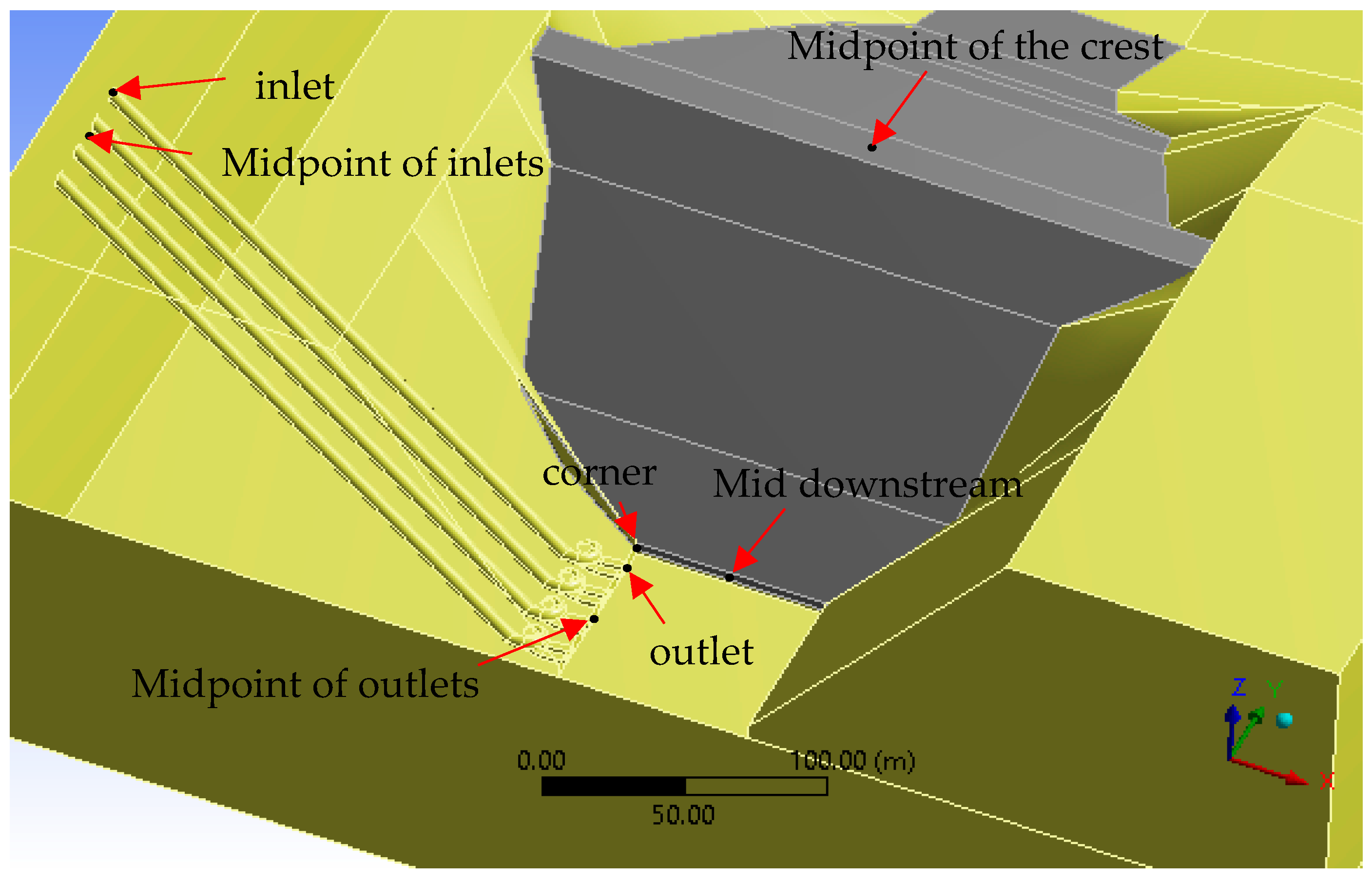
The steady flow boundary conditions computation is as follows. On the inlet of the turbine model at an elevation 245 m, the velocity was normal to inlet boundary. The initial value of the inlet velocity was determined by the flow rate listed in
Table 3. On the two rectangular outlets of the turbine model at 141 m elevation, the pressure (1 atmosphere) was determined according to the downstream water level.
The gradients of k and were assumed zero in the normal direction of boundaries except in the inlet boundary. The fixed wall and no-slip boundary conditions were applied. For the runner of the turbine rotating boundary, the runner periphery was moving at a velocity equal to the tangent velocity.
The results of the steady flow calculations were taken as the initial flow field for the complete unsteady flow passage. A time step of 0.001 s and runner rotating speeds of 3.1687 and 4.2671 rad/s were chosen for minimum and maximum upstream water levels, respectively, as shown in
Table 2. For each time step, the turbine runner rotated with angles of 1.53° and 1.5°, but for total time steps of 5000 s, the turbine runner should rotate more than one cycle.
The 3D numerical model was run to find the pressure boundary pattern by inputting the boundary conditions including the inlet velocity for minimum and maximum upstream water levels, rotational speed of turbines listed in
Table 3, outlet pressure (1 atmosphere), and the water properties. The turbine model was built in ANSYS-CFX and it is based on the finite volume technique. The flow simulation of the Francis turbine was employed by using several meshes to test the grid independence; it converged after many iterations. The grid independence of the turbine was created by using tetrahedral elements after performing several trials to determine the smallest possible aspect ratio under 150 and the minimum orthogonal over 0.15, as recommended by ANSYS-CFX code. The tetrahedron mesh was used because of its fine adaptability and the complexity of the computational domain. To obtain the required pressure fluctuation, the final mesh satisfied y
+ < 200 around the boundary wall, which is in agreement with the previous research conducted by Liu et al. [
48]. The runner, guide vanes, and draft tube interactions were counted using slip meshes. This slipping of meshes were toured around each other in the interface sides. However, it was important to ensure that the velocity components, pressure, and flow flux were harmonious after interpolation.
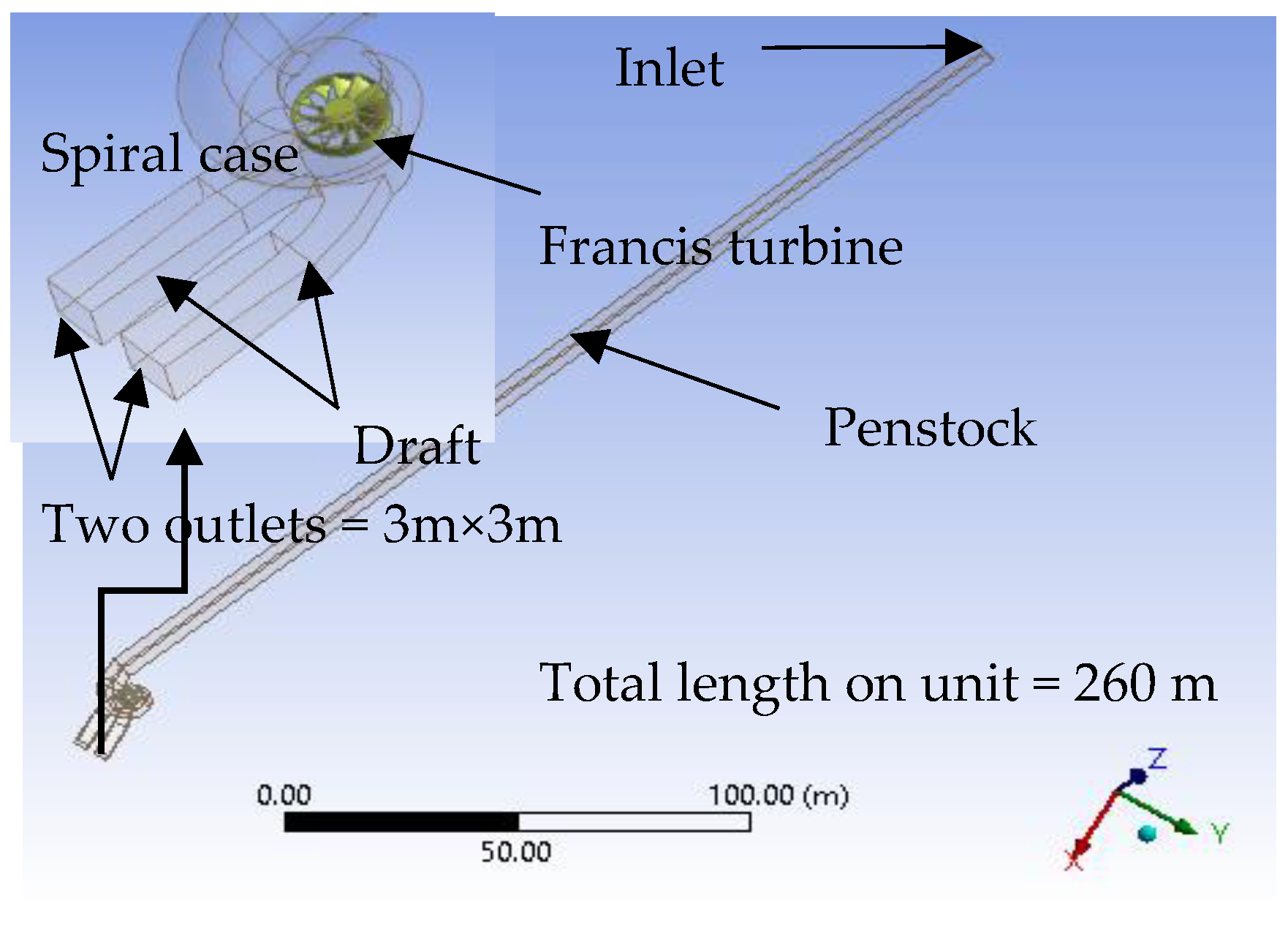
Table 4 shows the computational domain for the Temenggor Francis turbine model, which includes the 12 runner blades with the shaft, the Penstock, and the draft tubes. The total number of elements for the turbine model in the domain was 2.57 × 10
6, whereas the computational domain for the Temenggor dam model included a foundation of 127 m, upstream reservoir, with the concrete part including the spillway and the holes that represent the powerhouse region and the left and right embankments. The total number of cells for the turbine model in the domain was 1.93 × 10
6.
Based on turbine speed, we created numerous trails to determine the inlet pressure and determine the total head closest to the upstream water level. The total inlet head was estimated via the energy equation based on the sum of the velocity head, the elevation head, and the inlet pressure head results. This turbine model simulation represents the process used to determine the hydraulic performance of reaction turbines.
The water flows through the draft tube were modeled using the incompressible continuity formulation and Reynolds time average. The mathematical explanation can be presented as follows [
48]. The water flow continuity formula is:
The momentum formula is:
where:
The double formula of the
k-
is:
where
,
, and
.
can be determined:
where
,
4.38,
= 0.0845,
= 0.012,
= 1.42 “originally in the model procedure”,
= 1.68,
= 1.0, and
= 0.769. Among these constants used in the turbulence model, a properly chosen value of
was essential for improving the prediction of the pressure variation. In the present simulation,
= 1.45 was selected based on the preliminary computations.
6. Results and Discussion
The results obtained from the application of the 3D FE numerical model for the Temenggor dam integrated with the turbine model can be categorized into two summarized stages:
- (1)
The first stage of hydraulic performance results are related to the application of the 3D numerical finite volume turbine model by considering the operation of one vertical Francis turbine unit in the powerhouse of the Temenggor dam that was run in different water levels and discharge ranges. The results include velocity flow lines, pressure distribution in the turbines, and total estimated head at turbine inlet compared with the upstream water level.
- (2)
The second stage of the results were obtained from the integration of the 3D numerical finite element dam models with 3D numerical finite volume turbine models. The results cover all the possibilities that may arise from the operation of the powerhouses, including maximum and minimum water levels for the case of full inlet gates openings. The results of the 3D dam models include the principal stresses distributions in both dams and powerhouses.
6.1. Results of Turbine Numercal Models
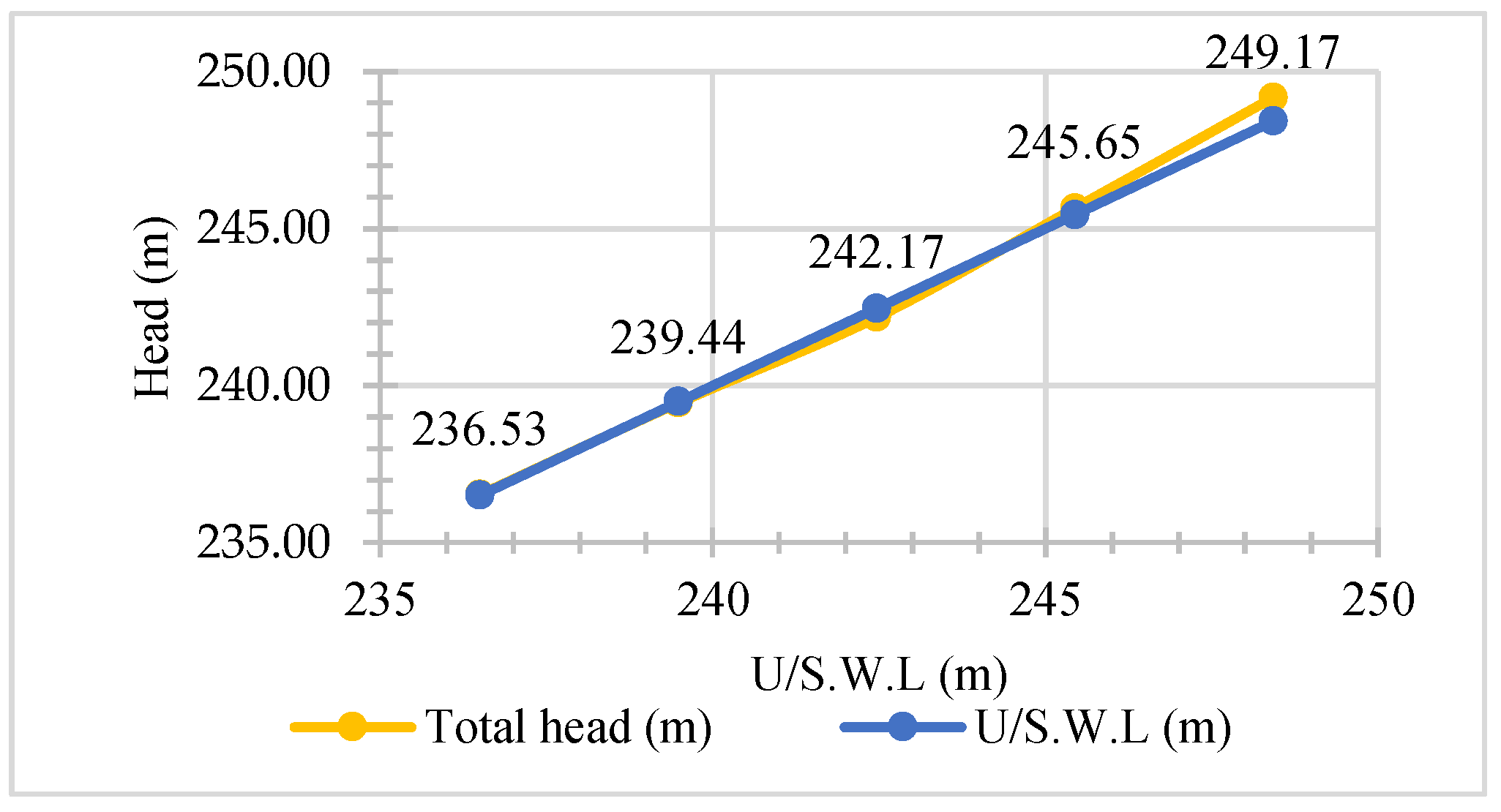
Table 6 outlines the calculations of the total head (H
t) at the inlet of the Temenggor turbine units depending on the inlet pressure model results. (v
2/2g) is the velocity head, (p/γ) is the pressure head, (Z) is the elevation head. Based on the turbine speed, we created numerous trails to determine the inlet pressure and determine the total head closest to the upstream water level. The total inlet head was estimated via the energy equation based on the sum of the velocity head, the elevation head, and the inlet pressure head results. This turbine model simulation represents the process used to determine the hydraulic performance of reaction turbines.
Figure 9 outlines the comparison between the total head estimated from numerical models with the upstream water levels. The results show that the maximum difference between the total head estimated from running the model and the upstream water level at the inlet of Temenggor turbine models was 0.75 m with an acceptable percent of error 0.3%.
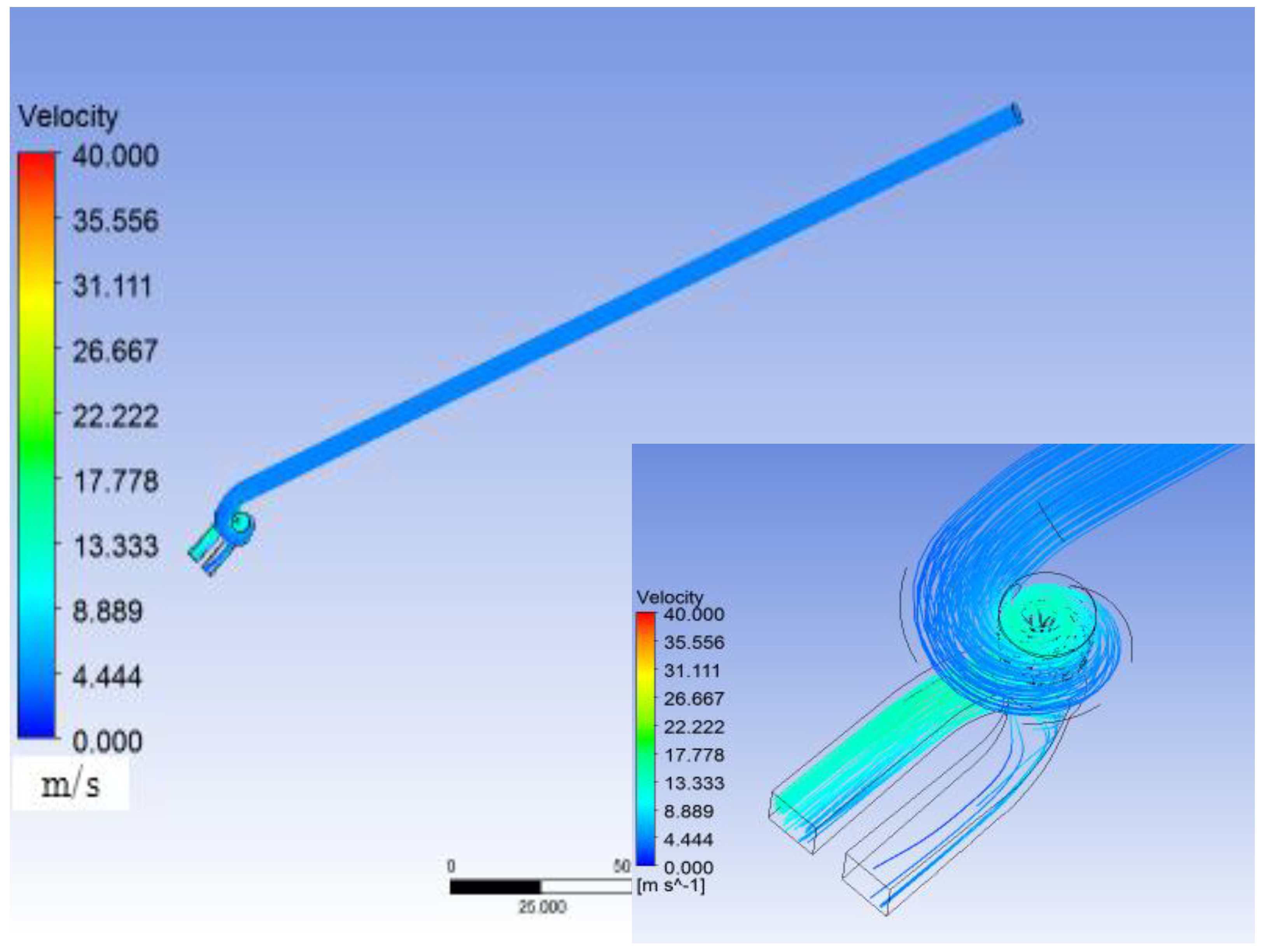
Figure 10 and
Figure 11 outline the velocity flow lines and boundary pressure distribution in Temenggor turbine units runs under maximum head. The velocity and pressure results were the closest in terms of distribution shape to the several studies reported in the literature [
44,
46,
49].
Velocity distribution along the penstock of the turbine model unit varied with the change in cross-sectional area. Based on the continuity equation and the cross-sectional area, the velocity gradually increased from the spiral case to the turbine runner. The velocity flow lines followed a spiral shape in the draft tube because of the rotational motion of the turbine runner. The results show that the maximum flow velocity occur at the runner region equal to 40 m/s at the 248.42 m upstream location.
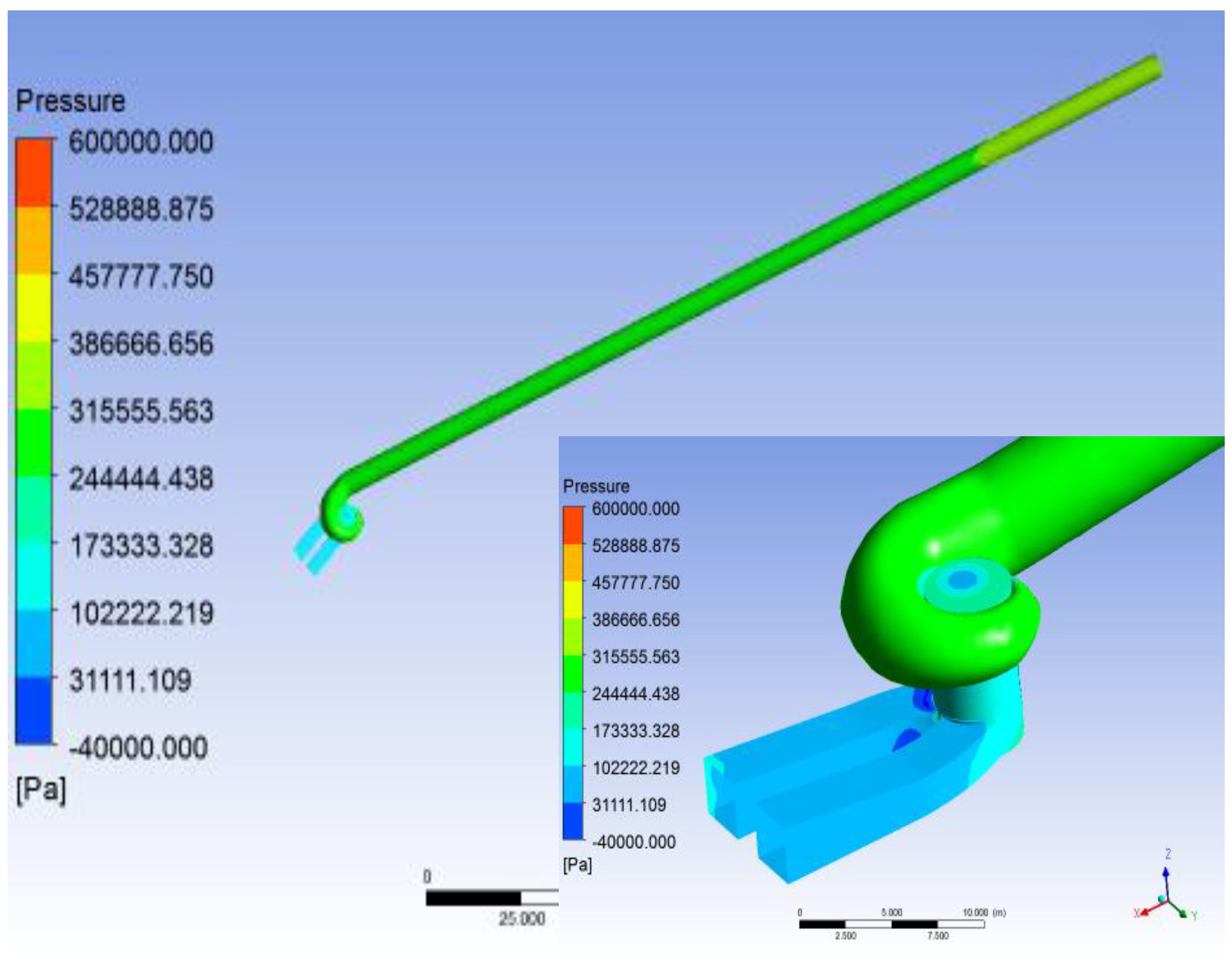
The boundary pressure distribution in the Temenggor Francis turbine units is shown in
Figure 11. It represents the case when the turbine runs under the flood upstream water levels. The results show that pressure distribution is proportional to the inverse of the velocity values based on the energy equation. However, the drop in pressure that occurs in the turbine shaft was more than the cavitation pressure. The pressure distribution and velocity flow lines are similar to those previously obtained [
49,
50].
6.2. Dynamic Analysis Results of Dam Model Connected with Turbine Model
The actual stress situation in the body of the dam is complex and may differ from the calculated stress state in the modeled design. The differences might be too high, leading to extensive dam damage. This inconsistency can be attributed to construction process, thermal stress during construction, operating period, water pressure in the reservoir, penetration of turbine outlets in dam body, base deformation, connections, and differences between actual values and predicted values of mechanical and thermal properties of materials. A comprehensive exploration of hydropower plant operation was conducted in order to reduce the principle stress on the dam structure. The finite element computation simulation and analysis were developed to investigate the optimal hydropower running with sustained long life of rock fill dam, with a case study of the Temenggor dam located in Malaysia.
The dam model was created to evaluate the principal stresses of the dam-turbine-reservoir-foundation system with changing water levels from maximum drawdown to the flood level. The fluid-solid connection, hydrostatic pressure, and gravity were defined. The latter was determined according to the water level and foundation depths.
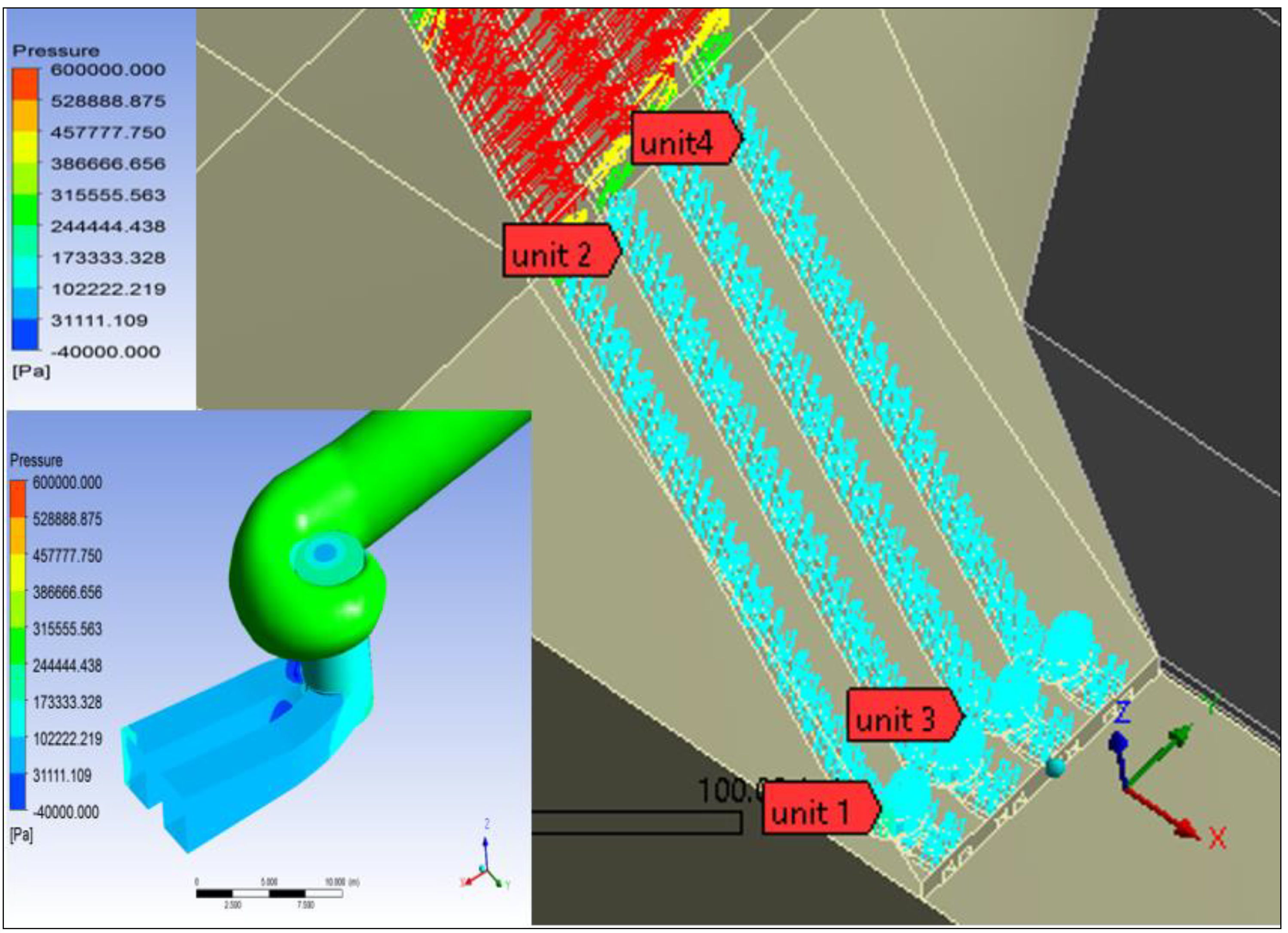
Figure 12 outlines the sequence and locations of the four turbine units in the Temenggor dams, with pressure distribution on the turbine units that transformed from turbine model to the dam body. The results show that the pressure decrease gradually from the inlet to the outlet of the units.
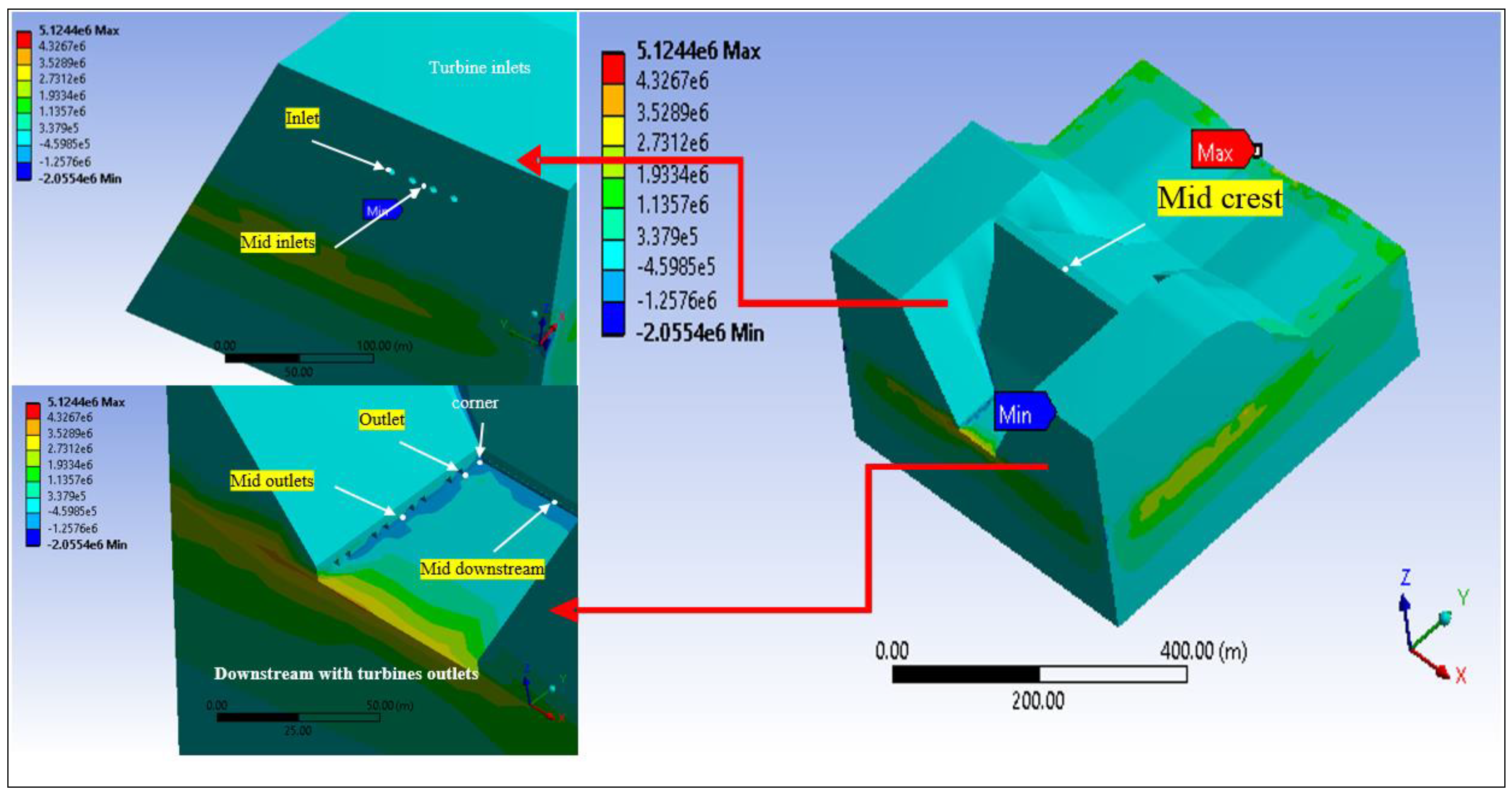
Figure 13 outlines the selected points for measuring the principle stress on the dam-reservoir-foundation system with a minimum water level with the effect of the four turbine units. The framework included two models: The Temenggor and Francis turbine model. ANSYS-CFX was used to model the transformation of the pressure to the dam model. ANSYS static structural facilities were used to convert the pressure from the turbine units to the common area between the dam and powerhouse for the purpose of simulating the principal stresses at selected locations (nodes) in the dam body. The modeling framework included 32 runs, in which 16 runs were performed with maximum water level in the reservoir and the other 16 runs were performed with minimum water level in the reservoir. These runs covered all possibilities of turbine operation.
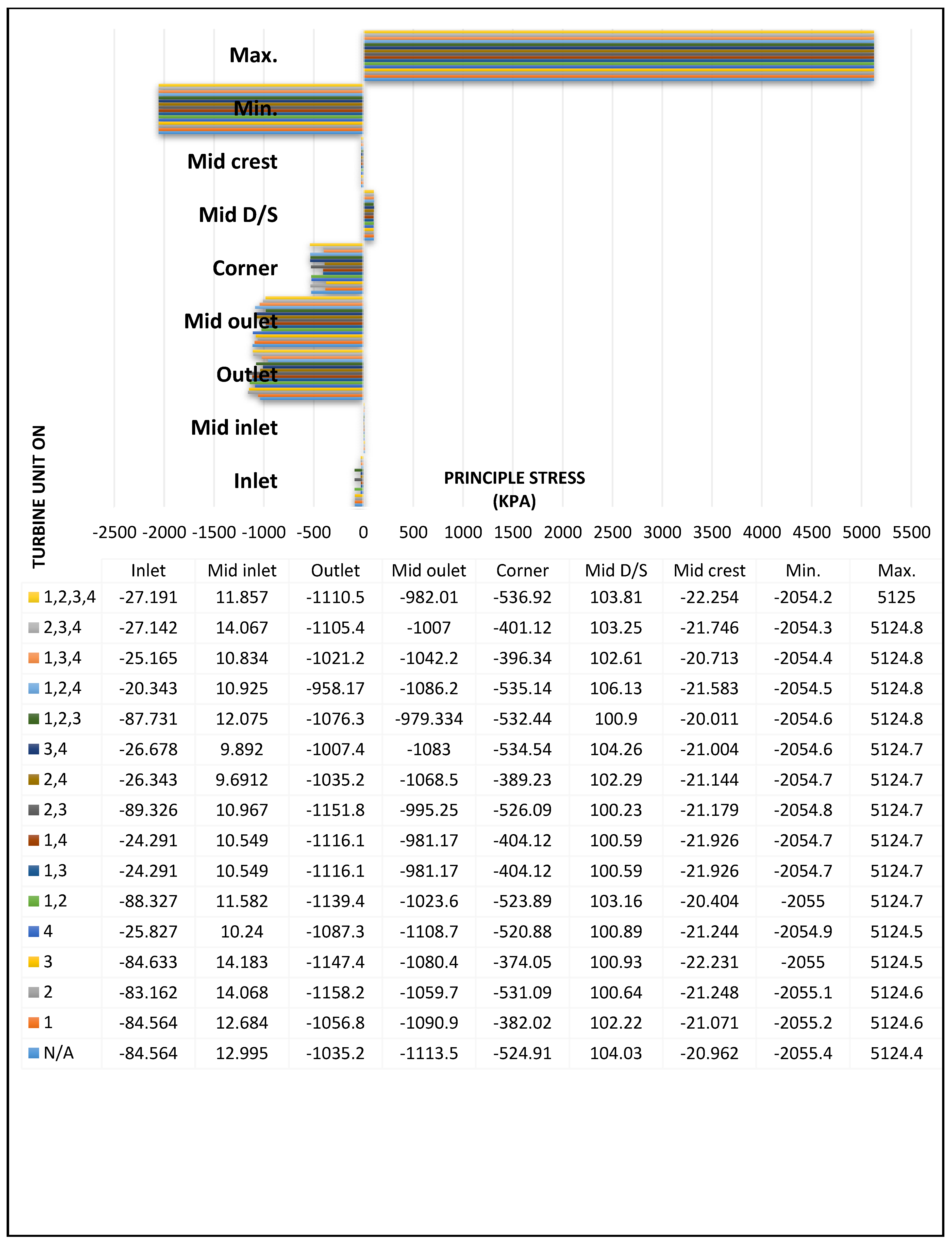
Figure 14 and
Figure 15 outline the principle stress results in the selected nodes shown in
Figure 13.
Table 7 and
Table 8 summarize the statistical analysis of the principle stress results.
Table 7 and
Table 8 show that the running of the powerhouse has a slight effect on the fluctuation of the maximum and minimum principle stress values and the percentage of change of these values are 0.01% and 0.06%, respectively. The points in the downstream near the outlet of the powerhouse are the most affected by the running turbines according to the fluctuation of the principle stress values (
Figure 13 and
Figure 14). The maximum range in principle stress change in the outlet occurs at maximum water level, which is equal to 200.03 kPa, and the maximum range in principle stress change in the mid outlet occurs with the minimum water level, which is equal to 144.9 kPa.
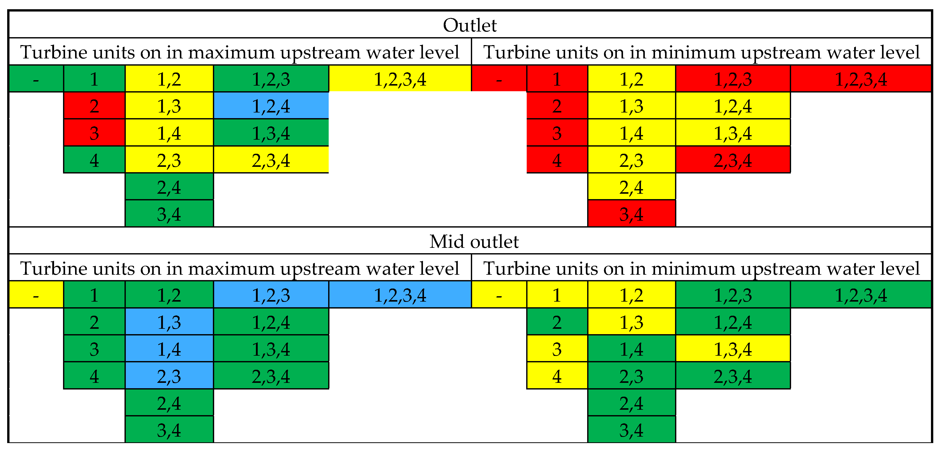
Table 9 outlines classifications according to the principle stress ranges in the outlet and mid outlet points to ensure the system worked with the minimum possible principle stress and to ensure the safety of the project and increase lifespan of the dam. Four colors were used to show the ranges in the principle stresses from minimum to maximum: blue, green, yellow, and red.
Figure 16 outlines a control program for the running turbines depending on the decrease in principle stress values in the selected points according to the classification listed in
Table 7. There were 32 total operation scenarios, with 16 operation scenarios based on maximum reservoir water level, and the other 16 operation scenarios were based on minimum reservoir water level.
The results from this study would help improve our current understanding of the consequences of the operation strategies imposed on the energy market, which tend to increase load variations, which in turn affects the lifespan of hydropower plant equipment. Therefore, the topic debated in this paper is more relevant and beneficial for the research of hydraulic and water resources in the engineering community.
8. Recommendation for Future Research
The motivation for conducting this research was to reduce the principle stresses and optimally operate a hydropower plan to obtain ideal dam operations and satisfy the primary fundamental aspects, such as safety and sustainability. In this research, a fully-opened gate was examined, so inspecting a partially opened gate is required, as this would be the usual case for the majority of the dams.
Due to the limitation of the ANSYS model, only one turbine unit can be operated in the simulation run and this is considered the major limitation of our modelling. This is reflected in the simulation runs where the pressure pattern obtained from running one turbine only was transfer to another turbine coordinates and then to the critical points on the dam body. Yet, studying the possibility of running all the turbines at the same time is more common in operating powerhouses. Another model with better capacity and facilities is recommended instead of the model used in this study. This may improve the accuracy of the simulation so better results can be obtained. Finally, it is advisable to conduct such studies on dam sites before construction so that the location of the power house can be carefully selected.


