Preliminary Study of Computational Time Steps in a Physically Based Distributed Rainfall–Runoff Model

Abstract

The choice of the computational time step (dt) value and the method for setting dt can have a bearing on the accuracy and performance of a simulation, and this effect has not been comprehensively researched across different simulation conditions. In this study, the effects of the fixed time step (FTS) method and the automatic time step (ATS) method on the simulated runoff of a distributed rainfall–runoff model were compared. The results revealed that the ATS method had less peak flow variability than the FTS method for the virtual catchment. In the FTS method, the difference in time step had more impact on the runoff simulation results than the other factors such as differences in the amount of rainfall, the density of the stream network, or the spatial resolution of the input data. Different optimal parameter values according to the computational time step were found when FTS and ATS were used in a real catchment, and the changes in the optimal parameter values were smaller in ATS than in FTS. The results of our analyses can help to yield reliable runoff simulation results.

1. Introduction

In the numerical analysis of water flows, the computational time step (dt) has mainly been studied from the perspective of a stable convergence of the solution. In practice, dt and control volume influence the stability and accuracy of a solution [1]. As the governing equation’s time difference step, a smaller value is used for dt than for the time steps of the input and output data. To set the dt during the simulation, a numerical model can use one of the following two approaches. The first is the fixed time step (FTS) method, in which the dt is fixed for the entire simulation, and the second is the automatic time step (ATS) method [1,2], in which the dt value is dynamically changed during the simulation. When FTS is used in the numerical model, the dt is set by the user. However, when ATS is used, only the initial value of the dt needs to be set, and the dt is automatically calculated normally using von Neuman stability conditions [3,4] or Courant–Friedrich–Lewy (CFL) conditions [5,6]. The von Neuman conditions use a Fourier series when performing finite difference analysis on a linear partial differential equation, and they are mainly employed in explicit solutions. The CFL conditions entail that the dt must be smaller than the time required for a given state’s wave to move through a distance of the control volume. The choice of the dt value and the method for setting dt can have a bearing on the accuracy and performance of the simulation, and this effect has not been comprehensively researched across different simulation conditions.

Normally, in a hydraulic model, the ATS method is employed to obtain a stable convergence of solution by changing the dt based on the flow volume and flow velocity which change during the flow simulation. For example, Kim et al. [7] evaluated the computational distance step and dt in a one-dimensional hydraulic model and proposed a method that estimates the variable computational distance step. Bates et al. [8] and Hunter et al. [2] evaluated the sensitivity to the initial value of the dt when using the ATS method, and they confirmed that, in comparison to the FTS method, the ATS method was able to obtain more accurate and stable computation results in a grid-based two-dimensional flood inundation analysis. When FTS is used in a hydrological model, the computed values of the peak flow and total runoff volume vary according to the dt [9]. Normally, when the dt is small, the peak flow and total runoff volume are larger than when the dt is large, and the time required for the runoff simulation becomes longer. Therefore, when the parameters are calibrated, the optimal parameter values vary depending on the dt. As a result, an optimal dt must be determined by comprehensively considering the appropriateness of the optimal parameter values and the time required for optimization.

For a numerical model to perform appropriate simulations, the FTS or the ATS method must be selected. To do this in an informed manner, it is necessary to adequately compare and evaluate the effect of these methods on the runoff simulation under simulation conditions such as the size of the control volume and the size of the discharge. However, existing studies on setting the dt mainly compare the computational results of FTS and ATS in terms of accuracy and have been focused on presenting methods for implementing the ATS method in a target model [1,2,10]. Sufficient research and information is not available regarding the effect that FTS and ATS have on computational results and model parameters with regard to the hydraulic and hydrological conditions of input data and the control volume conditions (e.g., grid size and grid properties).

The main objective of this study is to address this gap in the literature by conducting a detailed study on the effect that dt settings have on simulated flow in a variety of rainfall and catchment conditions. In particular, we analyze the variability of hydrological model computational results according to the choice of the FTS or ATS method and the virtual catchment’s simulation conditions. In the virtual catchment, the simulation conditions include the amount of rainfall, ratio of stream grids, and resolution of the control volume. We also use an optimization algorithm to calibrate parameters in real catchments to compare and evaluate the effect that each time step method (FTS or ATS) has on the variability of simulated hydrographs and optimized parameters. We use the grid-based rainfall–runoff model (GRM) [11] as a hydrological model, which is a physically based distributed rainfall–runoff model. The results and analyses contribute a detailed description of the effect of the choice of the dt value and the method used to set dt on the simulated runoff results in a variety of rainfall and catchment conditions. In particular, the results and analyses of this study on real catchments can help to obtain reasonable optimal parameter values and optimal flow simulation results for real catchments. The flow chart of this study is shown in Figure 1. To briefly describe the flow of this study, we first apply the FTS and ATS methods to the virtual catchment to compare whether the dt setting affects the peak flow for rainfall sizes. We then compare how the dt setting affects the peak flow for stream network densities. Third, we compare how much the dt setting affects the peak flow for spatial resolutions. Finally, we applied FTS and ATS methods to a real catchment to evaluate how much the dt setting affects simulated hydrographs and parameters.

2. Materials and Methods

2.1. GRM

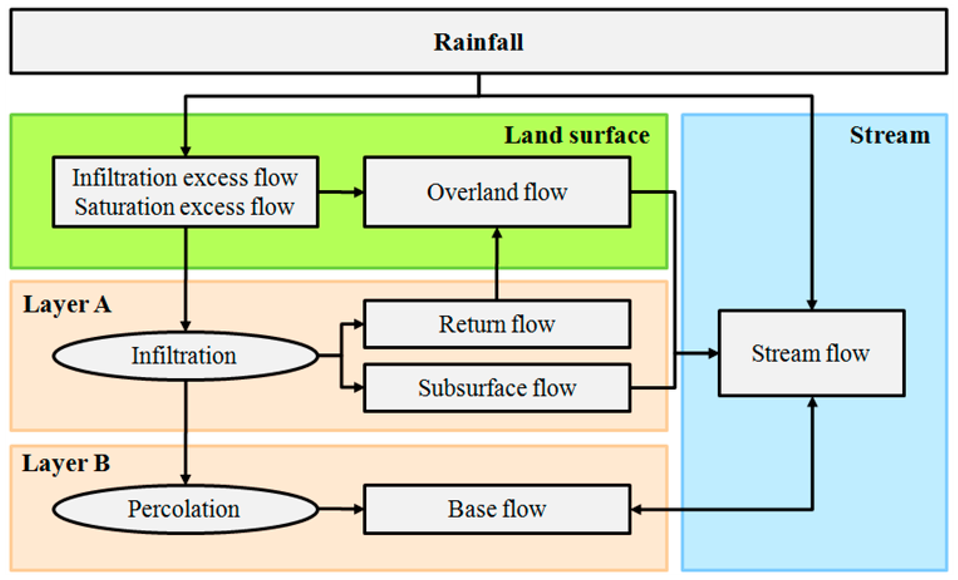
GRM is a physically based distributed rainfall–runoff model for simulating short-term rainfall events, and it can simulate surface and stream runoff, subsurface runoff, and baseflow (Figure 2). It uses a one-dimensional kinematic wave model for surface runoff and stream runoff simulation, and it uses the Green–Ampt model to calculate infiltration [11]. The governing equations of GRM are as follows.

$$\frac{\partial h}{\partial t}+\frac{\partial q}{\partial x}=r-f+\frac{q_r}{∆y}$$

(1)

$$\frac{\partial A}{\partial t}+\frac{\partial Q}{\partial x}=r∆y+q_L+q_{ss}+q_b$$

(2)

$$S_0=S_f$$

(3)

where h is flow depth, q (q = uh) is flow rate per unit width, u is overland flow velocity in the x direction, r is rainfall intensity, f is infiltration rate, q_r is return flow into the overland flow, ∆y is the width of control volume, A is the channel cross-sectional area, Q is the discharge in the channel, q_L is the lateral flow from overland flow, q_ss is subsurface flow, q_b is baseflow, S₀ is surface slope, and S_f is friction slope.

GRM can optionally use the FTS method or the ATS method, and when the ATS method is used, the dt is calculated via CFL conditions. For the theoretical specifics of GRM, refer to Choi and Kim [12].

2.2. CFL Condition

Because GRM simulates runoff by grid units, the distance of the control volume’s flow direction is the same as the resolution of the input spatial data. The CFL condition is shown in Equation (4). The distance of the control volume and the maximum velocity from the entire control volumes are used to calculate the maximum value of dt, which satisfies Equation (4). This dt value is used to perform a stable runoff simulation of the entire control volumes.

$$∆t\le \frac{∆x}{u_{max}}$$

(4)

where $u_{max}$ is the maximum value of the flow velocities for the entire grid calculated at time t, $∆t$ is the computational time step, and $∆x$ is the distance of the control volume’s flow direction.

2.3. Virtual Rainfall Events, Virtual Catchments and Analysis Method

The virtual rainfall events with properties described in

Table 1. Virtual rainfall events.

Virtual Rainfall Event Name	Max. Rainfall Intensity (mm/h)	Min. Rainfall Intensity (mm/h)	Total Rainfall (mm)	Rainfall Duration (h)
VR5	5	1	25	9
VR10	10	2	50
VR20	20	4	100
VR40	40	8	200

and the virtual catchments with properties described in

Table 2. Virtual domains.

Virtual Catchment Name	Catchment Area (km2)	Resolution	Slope (m/m)	Grid Number	Stream Grid		Applied Rainfall
					Number	Ratio * (%)
VD200_15	2540	200 m × 200 m	0.005	63,503	9250	15	VR20
VD200_9	2540	200 m × 200 m		63,503	5998	9	VR5, VR10, VR20, VR40
VD200_6	2540	200 m × 200 m		63,503	3744	6	VR20
VD500_10	2540	500 m × 500 m		10,201	996	10	VR20
VD1000_12	2540	1000 m × 1000 m		2550	295	12	VR20

* Ratio = (Stream grid number)/(Grid number) × 100.

were used to evaluate the effect of the method by which dt is set on the runoff for different virtual catchments and rainfall conditions. The virtual rainfall was 9 h of continuous rainfall with different intensities distributed over an isosceles triangle shape. The virtual catchments included five catchments with different resolutions and stream network densities. They have planar surfaces of same slope. The catchments were constructed with spatial resolutions of 200 m, 500 m, and 1000 m, and the stream network densities were between 6% and 15%. The slope of each virtual catchment was 0.005 m/m in all grids.

In the analysis of the virtual catchments, (1) four virtual rainfalls were applied to the VD200_9 virtual catchment to analyze how dt settings affect runoff according to rainfall conditions; (2) the VR20 rainfall was applied to three virtual catchments (VD200_15, VD200_9, VD200_6) with the same resolution but different stream network densities to analyze the effect of stream network density; (3) the VR20 virtual rainfall was applied to three virtual catchments (VD200_9, VD500_10, VD1000_12) with different spatial resolutions to analyze the effect of resolution.

2.4. Real Catchments, Real Rainfall Events and Analysis Method

To evaluate the effect of the method by which dt is set on the variability of the simulated flow and optimal parameters in a real catchment, the Danseong and Museong catchments in South Korea were chosen as target catchments (Figure 3 and

Table 3. Real catchments and rainfall events.

Catchment		Resolution	Rainfall		Observed Peak Flow (m3/s)
Name	Area (km2)		Period	Total Rainfall (mm)
Danseong	1709	500 m × 500 m	14 July 2012/15:00–21 July 2012/05:00	63	1213
Museong	472	200 m × 200 m	31 August 2007/20:00–02 September 2007/21:00	100	981

). The Danseong catchment’s area is 1709 km², and approximately 73% of the catchment is mountainous region. The Museong catchment’s area is 473 km², and approximately 87% of the catchment is mountainous region. Spatial data with a resolution of 500 m × 500 m were created for the Danseong catchment, and data with a resolution of 200 m × 200 m were created for the Museong region to be used as input data for GRM. One rainfall event was used for each of the catchments. Areal rainfall created by the Thiessen polygon method were used for the rainfall data. Note that the two catchments have a monsoon climate where there is a lot of rainfall in the summer for a long period of time.

In the analysis of the Danseong and Museong catchments, (1) the simulated flow according to the dt setting method was compared to the observed flow to evaluate its accuracy, and (2) an analysis was performed on the variability of the optimal parameter values which were calibrated by the shuffled complex evolution (SCE) algorithm [13,14] for each dt setting method. The SCE algorithm is a widely used parameter optimization algorithm [15] that is currently employed in a variety of fields [16,17,18,19,20]. Nash–Sutcliffe efficiency (NSE) [21] was used as the objective function for parameter optimization. NSE, normalized root mean square error (nRMSE), and the peak flow’s percentage error (PPE) were used as model performance evaluation statistics.

$$NSE=\frac{{{\displaystyle \sum }}_{i=1}^n{(Q_o^i-Q_s^i)}^2}{{{\displaystyle \sum }}_{i=1}^n{(Q_o^i-\overline{Q_o})}^2}$$

(5)

$$nRMSE=\frac{1}{Q_{max}-Q_{min}}\sqrt{\frac{{{\displaystyle \sum }}_{i=1}^n{(Q_o^i-Q_s^i)}^2}{n}}$$

(6)

$$PPE=\frac{\left|Q_{ps}-Q_{po}\right|}{Q_{po}}\times 100$$

(7)

where i is the order of the data, n is the total number of data, $Q_o^i$ is the observed flow, $Q_s^i$ is the simulated flow, $\overline{Q_o}$ is mean of the observed flow, $Q_{max}$ is maximum value of the observed flow, $Q_{min}$ is minimum value of the observed flow, $Q_{ps}$ is the simulated peak flow, and $Q_{po}$ is the observed peak flow. The parameters for calibration included the initial soil saturation ratio (ISSR), the minimum slope of channel bed (MSCB), the channel roughness coefficient (CRC), and the calibration coefficient of soil hydraulic conductivity (CCHC). The range of parameter values used in the SCE algorithm optimization was such that ISSR was 0–1, MSCB was 0.001–0.01, CRC was 0.008–0.2, and CCHC was 0.05–20.

3. Results and Discussion

3.1. Comparison of How Peak Flow is Affected by the dt Setting for Rainfall Size in a Virtual Catchment

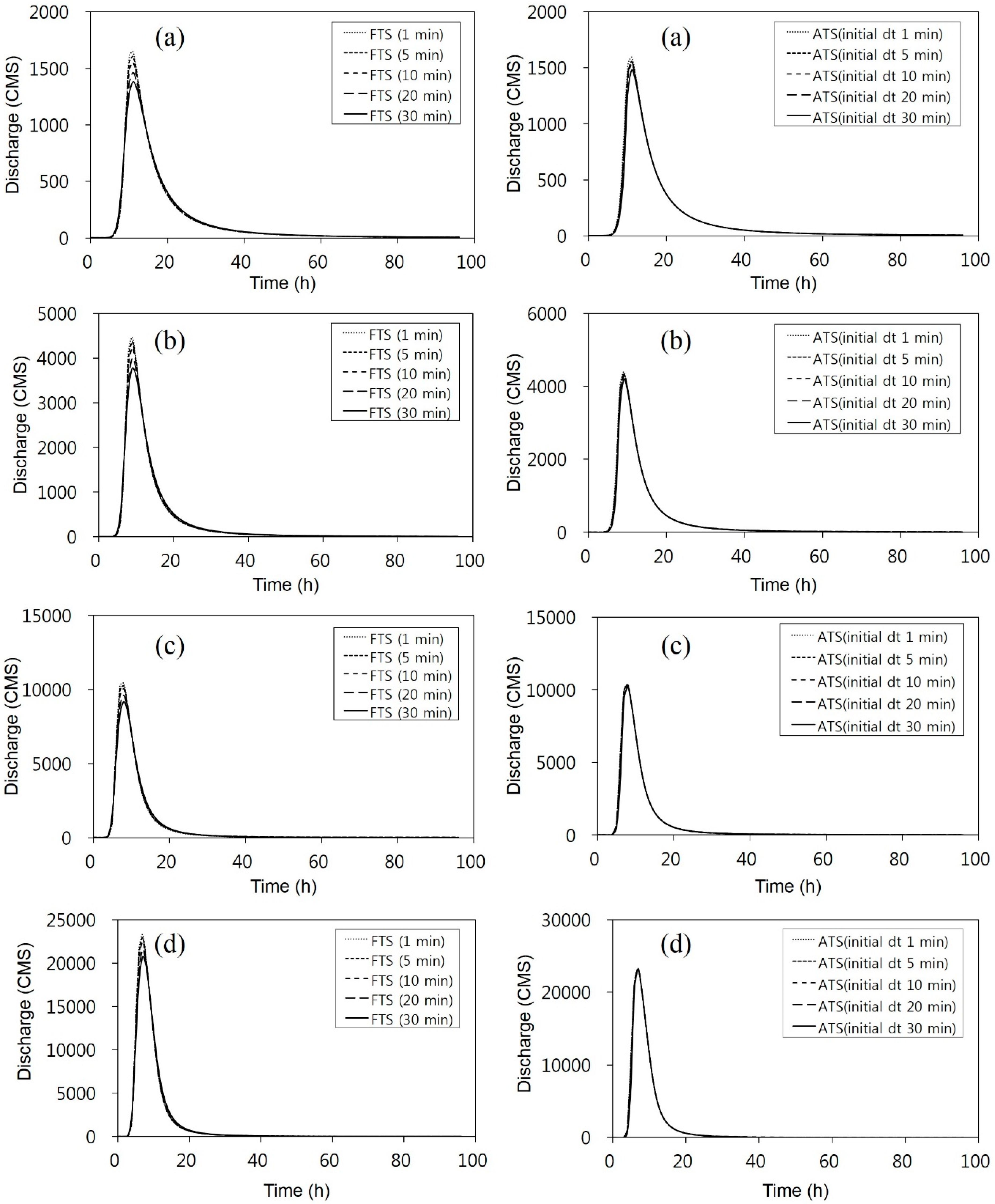
Rainfalls VR5, VR10, VR20, and VR40 were applied to the virtual catchment VD200_9, and the runoff hydrographs according to dt (FTS used a dt of 1, 5, 10, 20, and 30 min; ATS used these values as the initial dt) were compared (Figure 4 and

Table 4. Peak flows and peak flow’s percentage error (PPE) of VD200_9 using FTS and ATS.

Rainfall Event	FTS			ATS
	dt (min)	Peak Flow (m3/s)	PPE * (%)	Initial dt (min)	Peak Flow (m3/s)	PPE * (%)
VR5	1	1647	0	1	1596	0
	5	1605	3	5	1556	3
	10	1555	6	10	1537	4
	20	1462	11	20	1556	3
	30	1380	16	30	1476	8
VR10	1	4471	0	1	4395	0
	5	4367	2	5	4336	1
	10	4238	5	10	4276	3
	20	3995	11	20	4336	1
	30	3775	16	30	4186	5
VR20	1	10,427	0	1	10,354	0
	5	10,256	2	5	10,345	0
	10	10,039	4	10	10,269	1
	20	9603	8	20	10,345	0
	30	9182	12	30	10,187	2
VR40	1	23,323	0	1	23,288	0
	5	22,954	2	5	23,246	0
	10	22,497	4	10	23,202	0
	20	21,595	7	20	23,246	0
	30	20,720	11	30	23,129	1
Max. diff. PPE**	1		0	1		0
	5		1	5		2
	10		2	10		4
	20		4	20		3
	30		5	30		7

* PPE = Abs(B − A)/A × 100 where, A is peak flow when dt is 1 min and B is peak flow of each case. ** Max. diff. PPE: The maximum difference in PPE values for virtual rainfalls at each dt (For example, in the case of FTS dt = 30, it is 16 − 11 = 5).

). As there was no observed flow for the calculation of PPE for the virtual catchment in Table 4, the peak flow from when the dt was 1 min in each virtual rainfall was used as the observed flow. All the hydrographs in Figure 4 show similar simulation results except for the peak portion. The peak flows varied according to the dt values, and their differences became smaller as the amount of rainfall increased for both FTS and ATS. For example, at relatively small amounts of rainfall, such as for VR5 and VR10, FTS showed a maximum 16% PPE according to the dt value, and ATS showed a maximum of 8%. At relatively large amounts of rainfall, such as VR20 and VR40, FTS showed a maximum 12% PPE, and ATS showed a maximum of 2%. However, the changes in PPE according to changes in the amount of rainfall were a maximum of 5% for FTS and a maximum of 7% for ATS, indicating that changes in the amount of rainfall did not have a large effect on the changes in PPE for each dt value (see Max. diff. PPE in Table 4).

In a comparison of changes in peak flow according to the use of FTS and ATS, FTS showed a PPE that varied from 2% to 16% according to the dt value, and the dt value had a significant effect on the changes in the peak flow. However, ATS showed a PPE that varied from 1% to 8% according to the initial dt value; therefore, the changes in the peak flow in ATS were smaller than those in FTS. In addition, in FTS, when a dt of 5 min was used, a PPE of less than 3% was observed in all rainfall events. When a dt of 10 min was used, a maximum PPE of 6% was observed. However, when a dt of 20 min was used, a maximum PPE of 11% was observed, which showed a rapid increase in PPE. Therefore, when FTS was used, it was possible to simulate peak flow in a relatively stable way without regard to the amount of rainfall if a dt of less than 10 min was used. However, when ATS was used, a maximum PPE of 8% was seen during a small amount of rainfall (VR5), but in different amounts of rainfall, the PPE was always below 5% regardless of the initial dt value. Therefore, when ATS is used, a more stable peak flow can be simulated for any dt value than when FTS is used, regardless of the amount of rainfall.

3.2. Comparison of How Peak Flow is Affected by the dt Setting for Stream Network Density In Virtual Catchments

In GRM, the target of the stream runoff simulations is a grid that has river properties. In stream runoff, unlike surface runoff, the stream’s conveyance capacity affects the flow propagation, and the water depth and flow velocity are greater than in surface runoff. Therefore, the density of the grid that has river properties has a significant effect on the runoff simulation. This study evaluated the effect of the method by which the dt is set on the runoff, for different stream network densities (

Table 5. Peak flow and PPE for a virtual catchment with different stream grid ratios using FTS and ATS (VR20 was applied).

FTS								ATS
dt (min)	VD200_15		VD200_9		VD200_6		Max. diff. PPE *	Initial dt (min)	VD200_15		VD200_9		VD200_6		Max. diff. PPE
	Peak Flow (m3/s)	PPE	Peak Flow (m3/s)	PPE	Peak Flow (m3/s)	PPE			Peak Flow (m3/s)	PPE	Peak Flow (m3/s)	PPE	Peak Flow (m3/s)	PPE
1	10,762	0	10,427	0	9836	0	0	1	10,587	0	10,354	0	9663	0	0
5	10,434	3	10,256	2	9609	2	1	5	10,484	1	10,345	0	9579	1	1
10	10,193	5	10,039	4	9335	5	1	10	10,441	1	10,269	1	9489	2	1
20	9803	9	9603	8	8827	10	2	20	10,484	1	10,345	0	9579	1	1
30	9414	13	9182	12	8368	15	3	30	10,382	2	10,187	2	9281	4	2

* Max. diff. PPE: The maximum difference in PPE values of virtual catchments at each dt (For example, in the case of FTS dt = 30, it is 15 − 12 = 3).

). The VD200_15, VD200_9, and VD200_6 virtual catchments were used, and the ratios of each virtual catchment occupied by a stream grid were 15%, 9%, and 6%, respectively. VR20 was used as the virtual rainfall.

The results revealed that the maximum difference in PPE between stream networks with different densities for each dt value was a maximum of 3% in the case of FTS and 2% in the case of ATS (Table 5). Therefore, the PPE difference for each dt in the three virtual catchments with different stream network densities was not large. This indicates that stream network density does not have a large effect on changes in PPE.

3.3. Comparison of How Peak Flow is Affected by the dt Setting for Spatial Resolution in Virtual Catchments

To analyze how the dt settings affect the peak flow for different spatial resolutions, the VD200_9, VD500_10, and VD1000_12 virtual catchments were used. Each virtual catchment has a different spatial resolution, and their stream densities are 9%, 10%, and 12%. While VD200_9, VD500_10, and VD1000_12 have different stream network densities, in Section 3.2 it was found that stream network density does not have much effect on PPE. Therefore, we can use these virtual catchments to evaluate the effect that spatial resolution has on changes in PPE according to the dt value. VR20, which was used in Section 3.2, was used as the virtual rainfall.

The results revealed that the maximum difference in PPE between resolutions for each dt value was a maximum of 3% in the case of FTS and 5% in the case of ATS (

Table 6. Peak flow and PPE of each spatial resolution using FTS and ATS (VR20 was applied).

FTS								ATS
dt (min)	VD200_9		VD500_10		VD1000_12		Max. diff. PPE *	Initial dt (min)	VD200_9		VD500_10		VD1000_12		Max. diff. PPE
	Peak Flow (m3/s)	PPE	Peak Flow (m3/s)	PPE	Peak Flow (m3/s)	PPE			Peak Flow (m3/s)	PPE	Peak Flow (m3/s)	PPE	Peak Flow (m3/s)	PPE
1	10,427	0	8280	0	5619	0	0	1	10,354	0	8070	0	5379	0	0
5	10,256	2	8153	2	5546	1	1	5	10,345	0	7987	1	5338	1	1
10	10,039	4	7997	3	5456	3	1	10	10,269	1	7879	2	5108	5	4
20	9603	8	7693	7	5283	6	2	20	10,345	0	7987	1	5338	1	1
30	9182	12	7402	11	5115	9	3	30	10,187	2	7761	4	4999	7	5

* Max. diff. PPE: The maximum difference in PPE values of virtual catchments at each dt (For example, in the case of FTS dt = 30, it is 12 − 9 = 3).

), indicating that the PPE difference for the dt values in the three virtual catchments with different resolutions was not large. This implies that spatial resolution does not have a large effect on changes in PPE.

3.4. Evaluation of How Simulated Hydrographs and Parameters are Affected by dt Settings in Real Catchment

The FTS dt values and the ATS initial dt values used when calibrating parameters for the simulation in the real catchments were the same as in the virtual catchments at 1, 5, 10, 20, and 30 min. The parameter calibration results show that the changes in the simulated hydrographs were smaller for both the Danseong and Museong catchments when ATS was used than when FTS was used (Figure 5). In the Danseong catchment, the variability of the ATS method’s NSE, nRMSE, and PPE were markedly smaller than that of FTS (

Table 7. Statistics of simulated flow and calibrated parameters using different time steps.

Event	Items		FTS				ATS
			Min.	Max.	Ave.	Standard dev.	Min.	Max.	Ave.	Standard dev.
Danseong	Performance evaluation statistics	NSE	0.43	0.97	0.86	0.21	0.97	0.97	0.97	0.00
		nRMSE	0.05	0.24	0.10	0.07	0.05	0.06	0.05	0.00
		PPE	0.19	27.49	6.27	10.63	0.28	1.02	0.64	0.31
	Model parameters	ISSR	0.00	0.48	0.30	0.21	0.50	0.55	0.52	0.02
		MSCB	0.003	0.006	0.005	0.001	0.006	0.007	0.007	0.000
		CRC	0.191	0.200	0.196	0.003	0.185	0.199	0.193	0.005
		CCHC	7.72	14.60	12.78	2.56	13.21	13.77	13.49	0.21
Museong	Performance evaluation statistics	NSE	0.97	0.99	0.98	0.01	0.99	0.99	0.99	0.00
		nRMSE	0.03	0.04	0.04	0.00	0.03	0.03	0.03	0.00
		PPE	0.54	6.74	2.45	2.27	2.87	3.70	3.40	0.30
	Model parameters	ISSR	0.98	1.00	0.99	0.01	0.99	1.00	0.99	0.00
		MSCB	0.001	0.007	0.003	0.002	0.002	0.009	0.005	0.002
		CRC	0.072	0.169	0.112	0.031	0.081	0.186	0.133	0.036
		CCHC	0.87	1.84	1.31	0.40	1.64	1.86	1.79	0.08

NSE: Nash–Sutcliffe efficiency; ISSR: initial soil saturation ratio; MSCB: minimum slope of channel bed; CRC: channel roughness coefficient; CCHC: calibration coefficient of soil hydraulic conductivity.

). This implies that if ATS is used, the changes in the runoff simulation results caused by the dt setting are smaller than if FTS is used. In the Museong catchment, the changes in NSE, nRMSE, and PPE values were not large for FTS or ATS, but ATS showed lower variability in PPE than FTS.

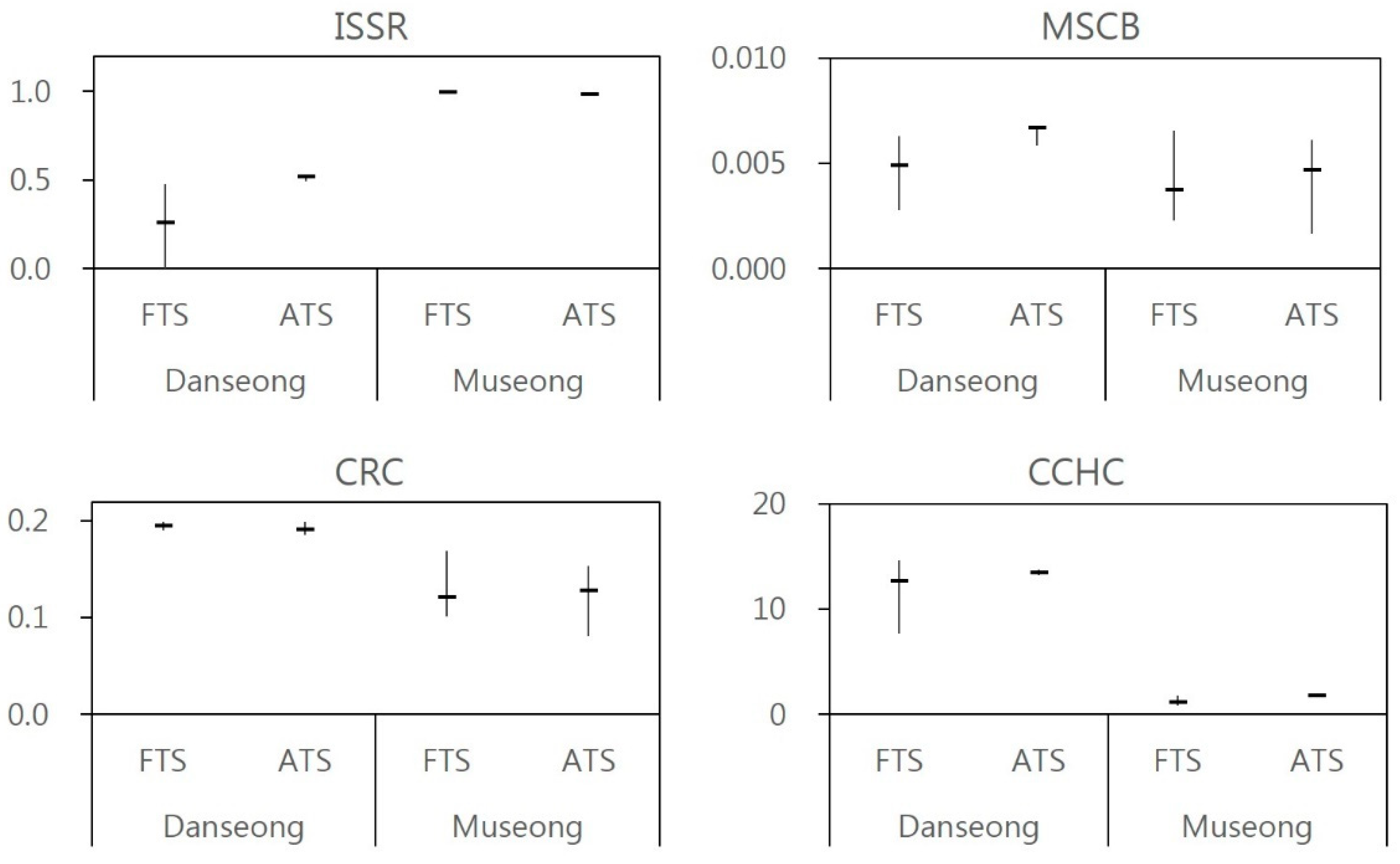
The parameter calibration results (Figure 6) showed that in the Museong catchment, the ranges of variability of all optimal parameter values were similar for FTS and ATS. However, in the Danseong catchment, the variability of ISSR, MSCB, and CCHC caused by the dt value was greater when FTS was used than when ATS was used. Like the virtual catchment results seen in Section 3.1, in FTS, there are large changes in the simulated flow when the dt varies (see PPE in Table 4), so there was a large range of changes in the optimal parameters during parameter optimization using different dt in the real catchments. This also means that in FTS, even if the parameters are optimized using the observed flow, at a certain dt value, it can be difficult to simulate the observed flow suitably (for example, dt = 30 min in Figure 5a). Note that the two catchments have a monsoon climate as mentioned in Section 2.4, so these results can be useful for catchments with monsoon climates. Since this study is about dt, these results can be applied to catchments with different climates, but care needs to be taken. Therefore, further studies on catchments with different climatic conditions are needed in the future.

4. Conclusions

This study used a physically based distributed rainfall–runoff model that is based on a kinematic wave model to comprehensively and quantitatively analyze the effect that dt settings have on simulated flow in a variety of rainfall and catchment conditions. In the analysis of the virtual catchment, changes in the dt value had a greater effect on changes in PPE when FTS was used than when ATS was used. When FTS was used, a relatively stable peak flow simulation was obtained when a dt of less than 10 min was used. Therefore, when FTS is used, the maximum value of the dt for obtaining the appropriate simulated flow value is 10 min under the rainfall and catchment conditions used in this study. In addition, when ATS was used, changes in the initial dt value did not have a significant effect on changes in PPE. The amount of rainfall, the stream network density, and the spatial resolution of input data did not have a considerable effect on changes in PPE for each dt. Therefore, the most important factor affecting the error in the simulated flow was the dt.

When runoff was simulated in real catchments using FTS, the changes in simulated flow and optimal parameter values due to the dt were larger than when ATS was used, and this phenomenon was more distinct in the Danseong catchment than in the Museong catchment. Therefore, when the dt value varies in FTS, the range of changes in the simulated runoff error and the range of changes in the optimal parameter values can vary according to the catchment. When ATS was used, the initial dt value had a small effect on changes in simulated flow and optimal parameter values for both catchments. This means that when ATS is used, stable runoff simulation results can be obtained regardless of the real catchment properties or the initial dt settings. Therefore, the results and analyses of this study on real catchments can help to obtain reasonable results for real-world practical applications. However, because this study used two real catchments, there is a limit to the generalizability of these results. Therefore, it is necessary to examine these results by applying this method to more real catchments in the future.

The results of this study show that by applying ATS rather than FTS, it is possible to obtain more valid and stable runoff simulation results when using a physically based distributed rainfall–runoff model based on a kinematic wave model. If the FTS method is used to simulate runoff, it is necessary to apply a variety of dt values to the target catchment and evaluate the validity of the model’s optimal parameters and simulated flow according to the dt values, and then use dt values that are suitable for the catchment.

References

1. Hulbert, G.M.; Jang, I. Automatic time step control algorithms for structural dynamics. Comput. Methods Appl. Mech. 1995, 126, 155–178. [Google Scholar] [CrossRef]
2. Hunter, N.M.; Horritt, M.S.; Bates, P.D.; Wilson, M.D.; Werner, M.G. An adaptive time step solution for raster-based storage cell modelling of floodplain inundation. Adv. Water. Resour. 2005, 28, 975–991. [Google Scholar] [CrossRef]
3. Charney, J.G.; Fjörtoft, R.; von Neumann, J. Numerical integration of the barotropic vorticity equation. Tellus 1950, 2, 237–254. [Google Scholar] [CrossRef]
4. Crank, J.; Nicolson, P. A practical method for numerical evaluation of solutions of partial differential equations of heat conduction type. Adv. Comput. Math. 1996, 6, 207–226. [Google Scholar] [CrossRef]
5. Courant, R.; Friedrichs, K.; Lewy, H. On the partial difference equations of mathematical physics. In AEC Research and Development Report, NYO-7689; AEC Computing and Applied Mathematics Centre: New York, NY, USA, 1956; pp. 63–76. [Google Scholar]
6. Scott, F.B.; Brett, F.S. Finite-Volume Model for Shallow-Water Flooding of Arbitrary Topography. J. Hydraul. Eng. 2002, 128, 289–298. [Google Scholar]
7. Kim, K.S.; Kim, J.S.; Kim, W. Estimation technique of computationally variable distance step in 1-D numerical model. KWRA 2011, 44, 363–376. (In Korean) [Google Scholar]
8. Bates, P.D.; Horritt, M.S.; Fewtrell, T.J. A simple inertial formulation of the shallow water equations for efficient two-dimensional flood inundation modelling. J. Hydrol. 2010, 387, 33–45. [Google Scholar] [CrossRef]
9. Haddeland, I.; Lettenmaier, D.P.; Skaugen, T. Reconciling simulated moisture fluxes resulting from alternate hydrologic model time steps and energy budget closure assumptions. J. Hydrometeorol. 2006, 7, 355–370. [Google Scholar] [CrossRef]
10. Givoli, D.; Henigsberg, I. A simple time-step control scheme. Commun. Numer. Methods Eng. 1993, 9, 873–881. [Google Scholar] [CrossRef]
11. Choi, Y.S.; Choi, C.K.; Kim, H.S.; Kim, K.T.; Kim, S. Multi-site calibration using a grid-based event rainfall–runoff model: A case study of the upstream areas of the Nakdong River basin in Korea. Hydrol. Process. 2015, 29, 2089–2099. [Google Scholar] [CrossRef]
12. Choi, Y.S.; Kim, K.T. Grid Based Rainfall-Runoff Model User’s Manual; Korea Institute of Civil Engineering and Building Technology: Goyang-si, Gyeonggi-do, Korea, 2017; pp. 1–21. [Google Scholar]
13. Duan, Q.Y.; Gupta, V.K.; Sorooshian, S. Shuffled complex evolution approach for effective and efficient global minimization. J. Optim. Theory Appl. 1993, 76, 501–521. [Google Scholar] [CrossRef]
14. Duan, Q.; Sorooshian, S.; Gupta, V. Effective and efficient global optimization for conceptual rainfall-runoff models. Water Resour. Res. 1992, 28, 1015–1031. [Google Scholar] [CrossRef]
15. Nicklow, J.; Reed, P.; Savic, D.; Dessalegne, T.; Harrell, L.; Chan-Hilton, A.; Karamouz, M.; Minsker, B.; Ostfeld, A.; Singh, A.; et al. State of the art for genetic algorithms and beyond in water resources planning and management. J. Water Res. Plan. Manag. 2010, 136, 412–432. [Google Scholar] [CrossRef]
16. Moreno, H.A.; Vivoni, E.R.; Gochis, D.J. Utility of quantitative precipitation estimates for high resolution hydrologic forecasts in mountain watersheds of the Colorado Front Range. J. Hydrol. 2012, 438, 66–83. [Google Scholar] [CrossRef]
17. Serrat-Capdevila, A.; Scott, R.L.; Shuttleworth, W.J.; Valdés, J.B. Estimating evapotranspiration under warmer climates: Insights from a semi-arid riparian system. J. Hydrol. 2011, 399, 1–11. [Google Scholar] [CrossRef]
18. Shin, M.J.; Eum, H.I.; Kim, C.S.; Jung, I.W. Alteration of hydrologic indicators for Korean catchments under CMIP5 climate projections. Hydrol. Process. 2016, 30, 4517–4542. [Google Scholar] [CrossRef]
19. Shin, M.J.; Guillaume, J.H.; Croke, B.F.; Jakeman, A.J. A review of foundational methods for checking the structural identifiability of models: Results for rainfall-runoff. J. Hydrol. 2015, 520, 1–16. [Google Scholar] [CrossRef]
20. Shin, M.J.; Kim, C.S. Assessment of the suitability of rainfall–runoff models by coupling performance statistics and sensitivity analysis. Hydrol. Res. 2017, 48, 1192–1213. [Google Scholar] [CrossRef]
21. Nash, J.E.; Sutcliffe, J.V. River flow forecasting through conceptual models part I—A discussion of principles. J. Hydrol. 1970, 10, 282–290. [Google Scholar] [CrossRef]
Figure 1. Flow chart of this study.
Water 10 01269 g001
Figure 2. Flow diagram of the grid-based rainfall–runoff model (GRM) [12].
Water 10 01269 g002
Figure 3. Study area. (a) Danseong catchment; and (b) Museong catchment.
Water 10 01269 g003
Figure 4. Hydrographs for different dts from virtual rainfall events for VD200_9 using a fixed time step (FTS) and automatic time step (ATS). (a) are hydrographs from VR5; (b) are hydrographs from VR10; (c) are hydrographs from VR20; and (d) are hydrographs from VR40.
Water 10 01269 g004
Figure 5. Hydrographs using FTS and ATS. (a) Danseong catchment; and (b) Museong catchment.
Water 10 01269 g005
Figure 6. Minimum, maximum, and average values of calibrated model parameters using different time steps. The (⚊) mark indicates the average value.
Water 10 01269 g006