SWB Modeling of Groundwater Recharge on Catalina Island, California, during a Period of Severe Drought


Abstract
:1. Introduction
2. Materials and Methods
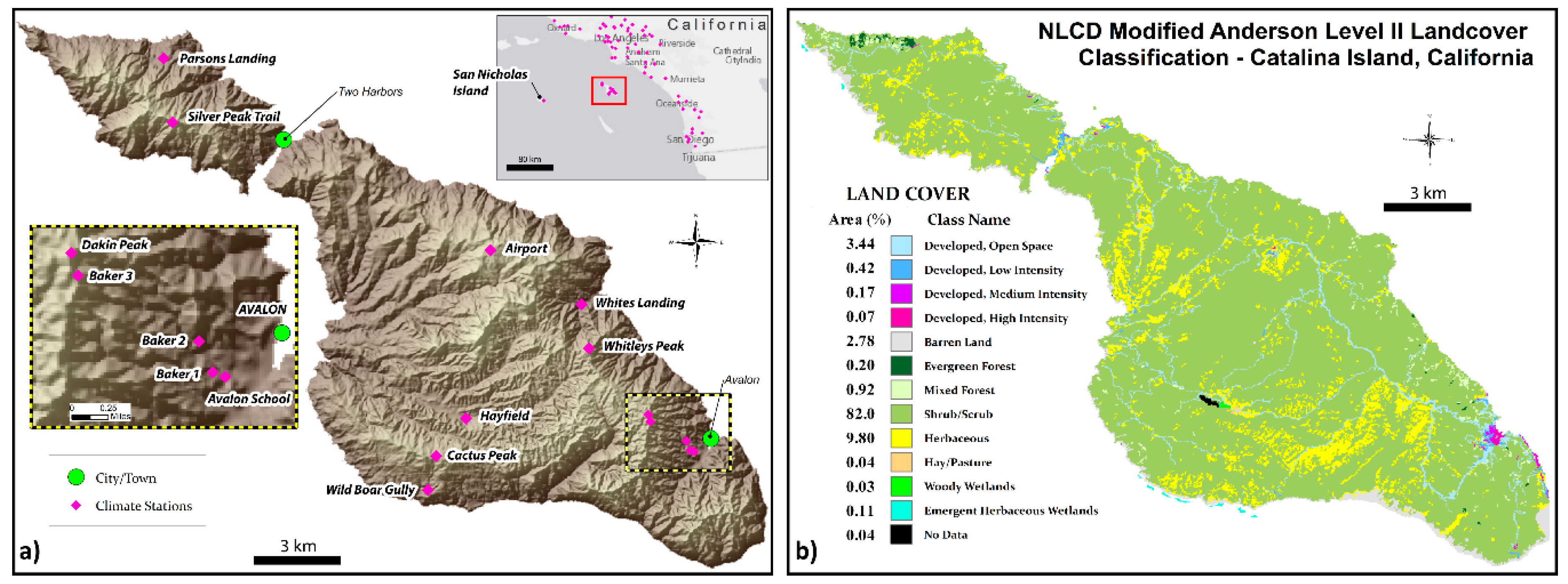
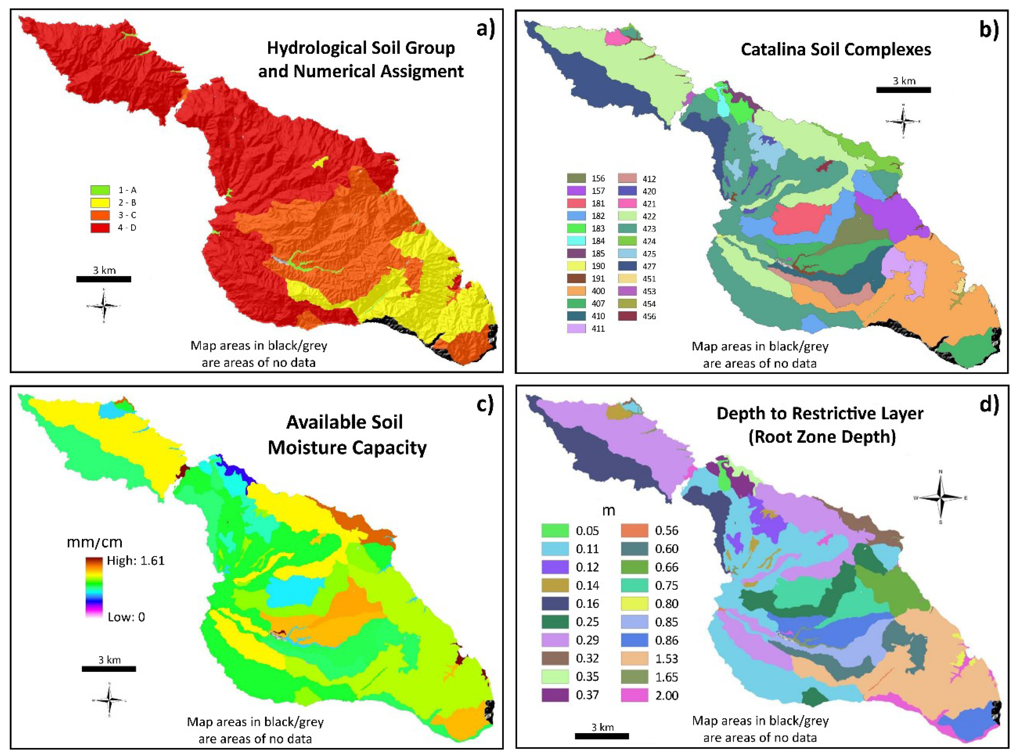
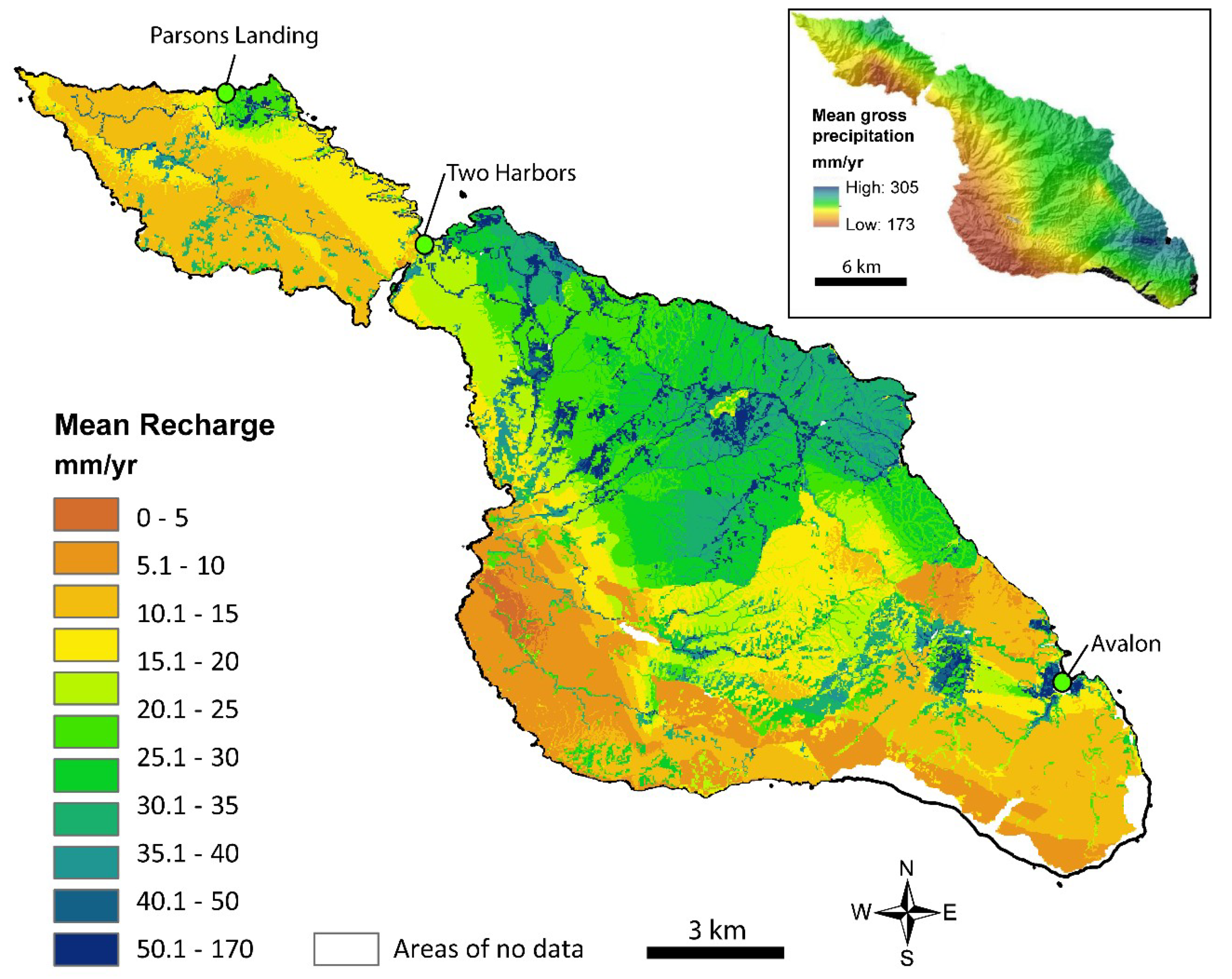
2.1. Study Area
2.2. The SWB Model
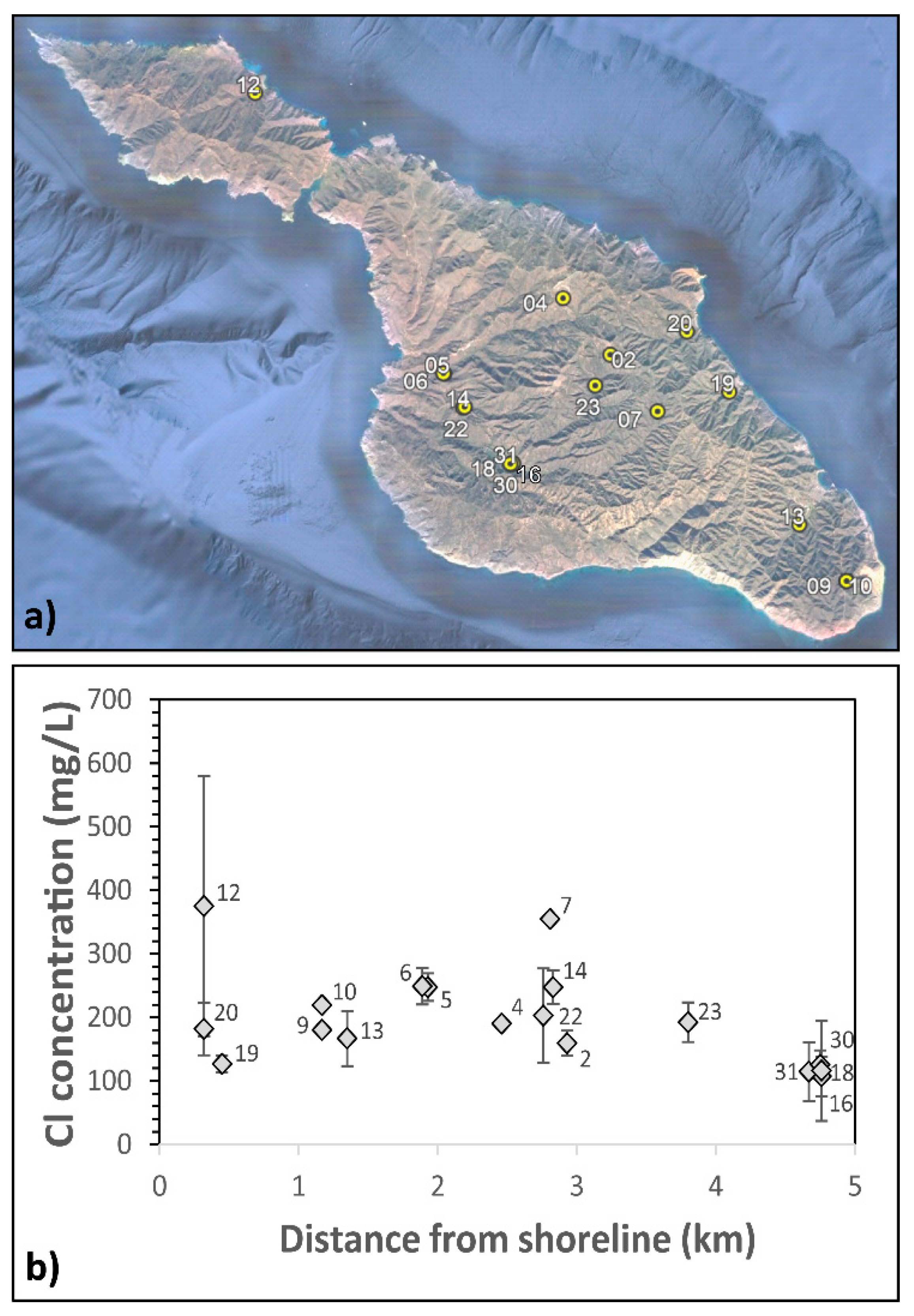
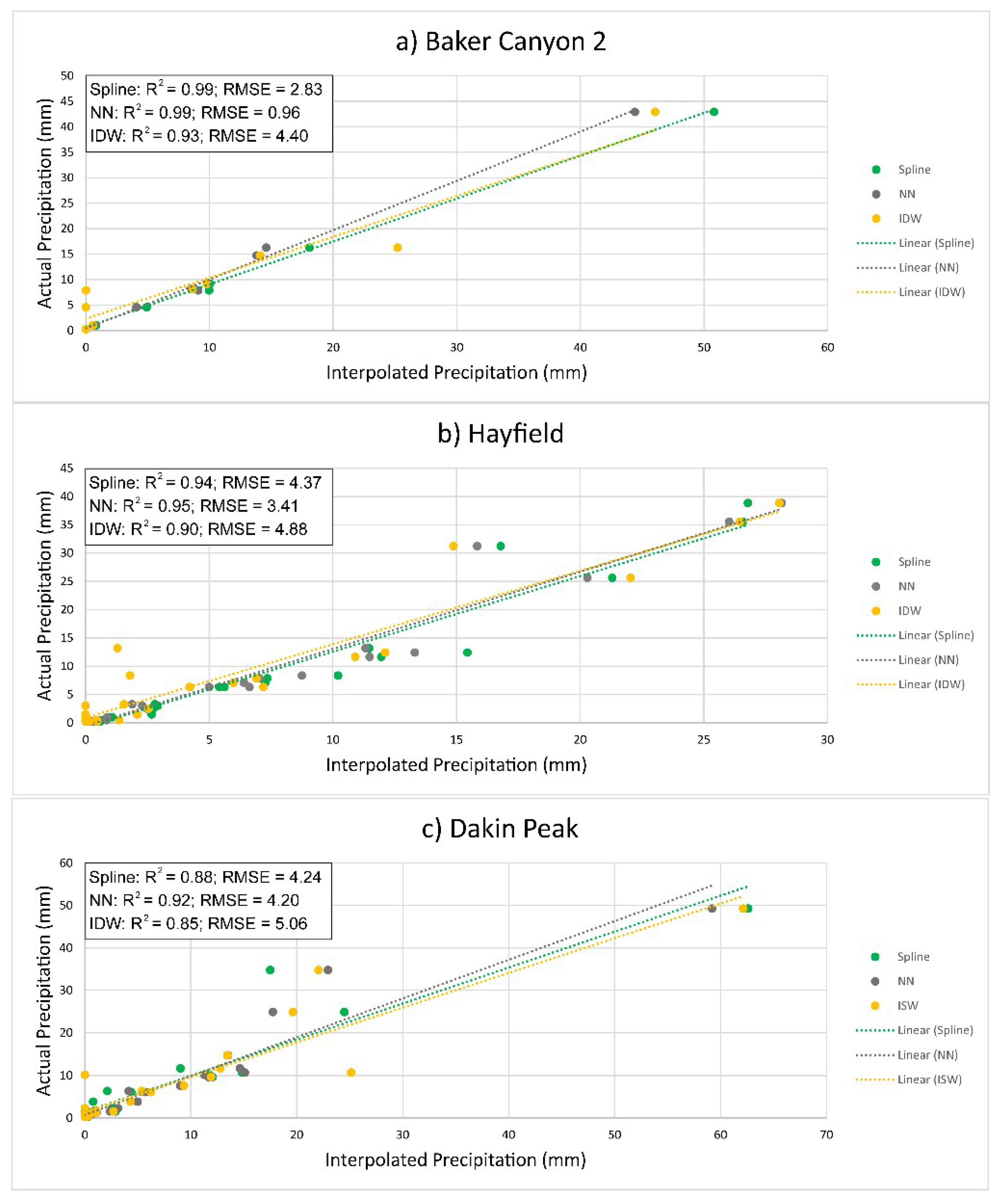
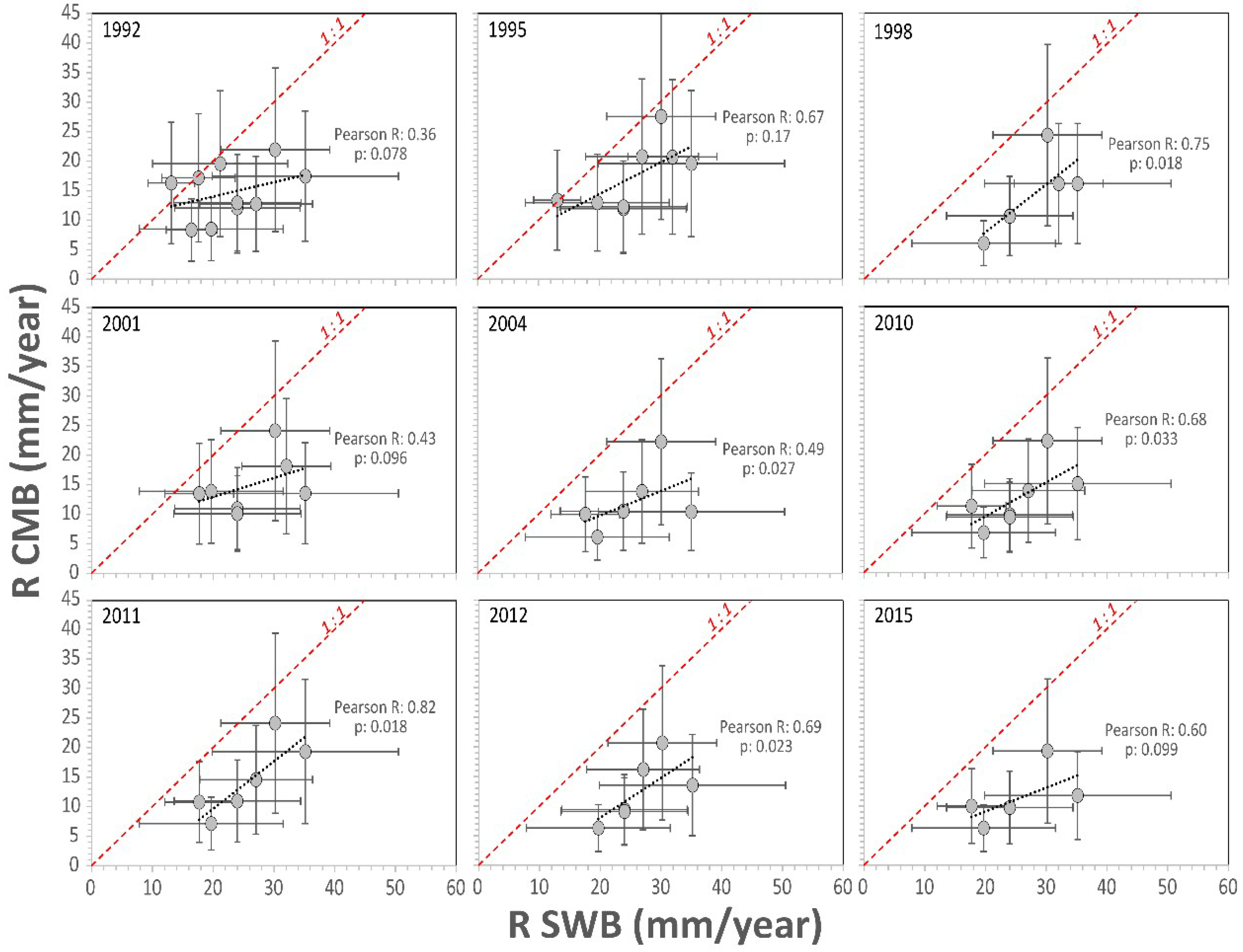
2.3. Corroboration of Recharge Estimates
3. Results and Discussion
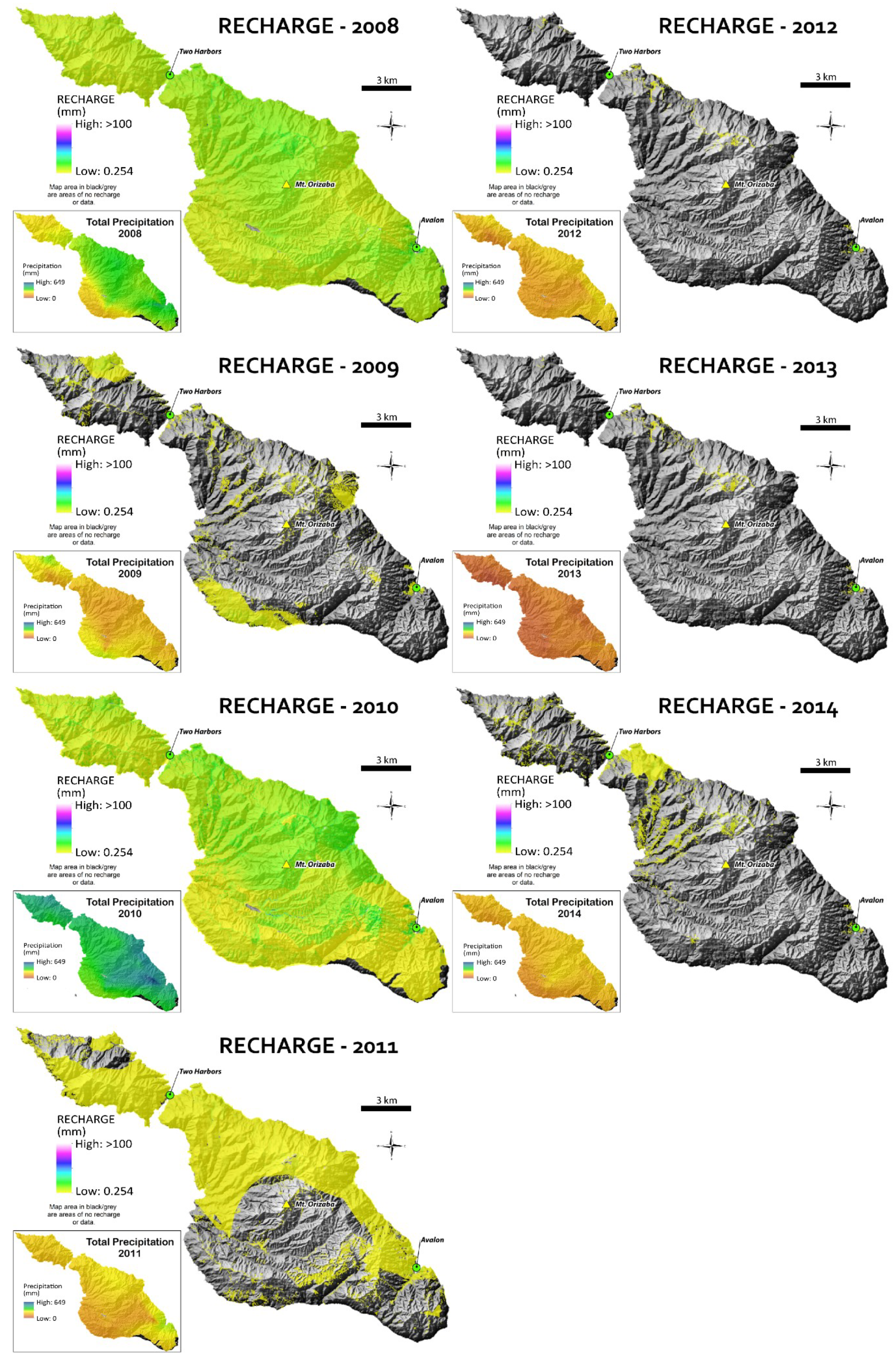
3.1. SWB Recharge Output
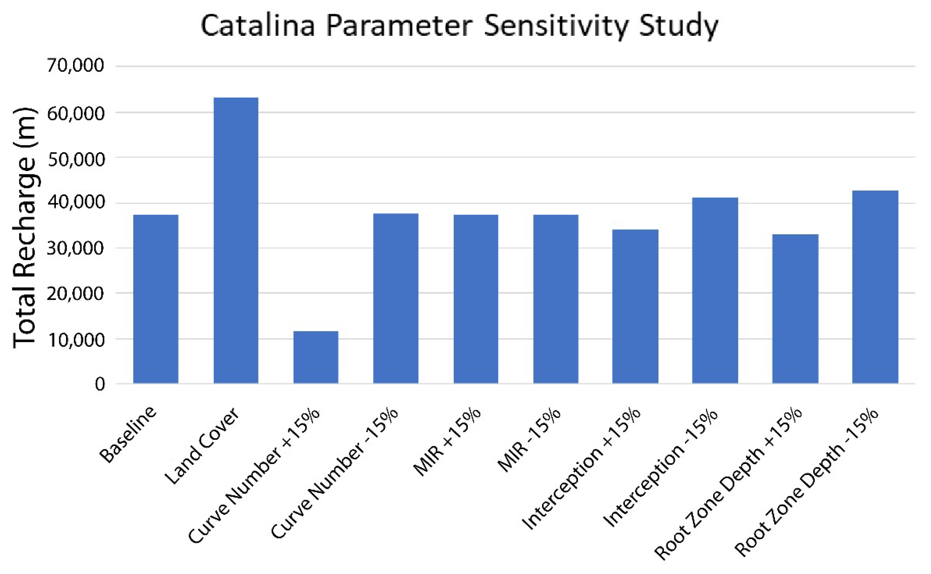
3.2. Sensitivity Analysis
3.3. Limitations of Study
4. Conclusions and Implications
Author Contributions
Funding
Acknowledgments
Conflicts of Interest
References
- McMahon, P.B.; Plummer, L.N.; Boehlke, J.K.; Shapiro, S.D.; Hinkle, S.R. A comparison of recharge rates in aquifers of the United States based on groundwater-age data. Hydrogeol. J. 2011, 19, 779–800. [Google Scholar] [CrossRef]
- Castle, S.L.; Thomas, B.F.; Reager, J.T.; Rodell, M.; Swenson, S.C.; Famiglietti, J.S. Groundwater Depletion during Drought Threatens Future Water Security of the Colorado River Basin. Geophys. Res. Lett. 2014, 41, 5904–5911. [Google Scholar] [CrossRef] [PubMed]
- Service, R.F. California’s Water Crisis: Worse to Come? Science 2009, 323, 1665. [Google Scholar] [CrossRef] [PubMed]
- Thomas, B.F.; Caineta, J.; Nanteza, J. Global Assessment of Groundwater Sustainability Based on Storage Anomalies. Geophys. Res. Lett. 2017, 44. [Google Scholar] [CrossRef]
- Chen, X.; Zhang, Z.-C.; Zhang, X.-N.; Chen, Y.-Q.; Qian, M.-K.; Peng, S.-F. Estimation of Groundwater Recharge from Precipitation and Evapotranspiration by Lysimeter Measurement and Soil Moisture Model. J. Hydrol. Eng. 2008, 13, 333–340. [Google Scholar] [CrossRef]
- Crosbie, R.S.; Binning, P.; Kalma, J.D. A time series approach to inferring groundwater recharge using the water table fluctuation method. Water Resour. Res. 2005, 41. [Google Scholar] [CrossRef] [Green Version]
- Hagedorn, B. Hydrochemical and 14C constraints on groundwater recharge and interbasin flow in an arid watershed: Tule Desert, Nevada. J. Hydol. 2015, 523, 297–308. [Google Scholar] [CrossRef]
- Healy, R.W.; Cook, P.G. Using groundwater levels to estimate recharge. Hydrogeol. J. 2002, 10, 91–109. [Google Scholar] [CrossRef]
- Somaratne, N. Characteristics of Point Recharge in Karst Aquifers. Water 2014, 6, 2782–2807. [Google Scholar] [CrossRef] [Green Version]
- Von Freyberg, J.; Moeck, C.; Schirmer, M. Estimation of groundwater recharge and drought severity with varying model complexity. J. Hydrol. 2015, 527, 844–857. [Google Scholar] [CrossRef]
- Izbicki, J.A.; Stamos, C.L.; Nishikawa, T.; Martin, P. Comparison of ground-water flow model particle-tracking results and isotopic data in the Mojave River ground-water basin, southern California, USA. J. Hydrol. 2004, 292, 30–47. [Google Scholar] [CrossRef]
- McCoy, K.J.; Yager, R.M.; Nelms, D.L.; Ladd, D.E.; Monti, J., Jr.; Kozar, M.D. Hydrologic Budget and Conditions of Permian, Pennsylvanian, and Mississippian Aquifers in the Appalachian Plateaus Physiographic Province; U.S. Geological Survey Scientific Investigations Report 2015–5106; U.S. Geological Survey: Reston, VA, USA, 2015; p. 77.
- Moreno, H.A.; Gupta, H.V.; White, D.D.; Sampson, D.A. Modeling the distributed effects of forest thinning on the long-term water balance and streamflow extremes for a semi-arid basin in the southwestern US. Hydrol. Earth Syst. Sci. 2016, 20, 1241–1267. [Google Scholar] [CrossRef] [Green Version]
- Sanford, W. Recharge and groundwater models: An overview. Hydrogeol. J. 2002, 10, 110–120. [Google Scholar] [CrossRef]
- Smith, E.A.; Westenbroek, S.M. Potential Groundwater Recharge for the State of Minnesota Using the Soil-Water-Balance Model, 1996–2010; U.S. Geological Survey Scientific Investigations Report 2015-5038; U.S. Geological Survey: Reston, VA, USA, 2015; p. 85.
- Hagedorn, B.; El-Kadi, A.I.; Mair, A.; Whittier, R.B.; Ha, K. Estimating recharge in fractured aquifers of a temperate humid to semiarid volcanic island (Jeju, Korea) from water table fluctuations, and Cl, CFC-12 and 3H chemistry. J. Hydrol. 2011, 409, 650–662. [Google Scholar] [CrossRef]
- Gehman, C.L.; Harry, D.L.; Sanford, W.E.; Stednick, J.D.; Beckman, N.A. Estimating specific yield and storage change in an unconfined aquifer using temporal gravity surveys. Water Resour. Res. 2009, 45. [Google Scholar] [CrossRef] [Green Version]
- Somaratne, N. Pitfalls in application of the conventional chloride mass balance (CMB) in karst aquifers and use of the generalised CMB method. Environ. Earth Sci. 2015, 74, 337–349. [Google Scholar] [CrossRef]
- Hagedorn, B.; Clarke, N.; Ruane, M.; Faulkner, K. Assessing aquifer vulnerability from lumped parameter modeling of modern water proportions in groundwater mixtures: Application to California’s South Coast Range. Sci. Total Environ. 2018, 624, 1550–1560. [Google Scholar] [CrossRef] [PubMed]
- Jurgens, B.C.; Boehlke, J.K.; Kauffman, L.J.; Belitz, K.; Esser, B.K. A partial exponential lumped parameter model to evaluate groundwater age distributions and nitrate trends in long screened wells. J. Hydol. 2017, 543, 109–126. [Google Scholar] [CrossRef]
- Koh, D.-C.; Chang, H.-W.; Lee, K.-S.; Ko, K.-S.; Kim, Y.; Park, W.-B. Hydrogeochemistry and environmental isotopes of ground water in Jeju volcanic island, Korea: Implications for nitrate contamination. Hydrol. Process. 2005, 19, 2225–2245. [Google Scholar] [CrossRef]
- Zhu, C. Estimate of recharge from radiocarbon dating of groundwater and numerical flow and transport modeling. Water Resour. Res. 2000, 36, 2607–2620. [Google Scholar] [CrossRef] [Green Version]
- USGS. Documentation of Computer Program INFIL3.0—A Distributed Parameter Watershed Model to Estimate Net Infiltration below the Root Zone; U.S. Geological Survey Scientific Investigations Report 2008-5006; U.S. Geological Survey: Reston, VA, USA, 2008; p. 98.
- Oki, D.S. The Significance of Accounting Order for Evapotranspiration and Recharge in Monthly and Daily Threshold-Type Water Budgets; U.S. Geological Survey Scientific Investigations Report 2008-5163; U.S. Geological Survey: Reston, VA, USA, 2008.
- Jasechko, S.; Taylor, R.G. Intensive rainfall recharges tropical groundwaters. Environ. Res. Lett. 2015, 10, 124015. [Google Scholar] [CrossRef] [Green Version]
- Scanlon, B.R.; Healey, R.W.; Cook, P.G. Choosing appropriate techniques for quantifying groundwater recharge. Hydrogeol. J. 2002, 10, 18–39. [Google Scholar] [CrossRef]
- Westenbroek, S.M.; Kelson, V.A.; Dripps, W.R.; Hunt, R.J.; Bradbury, K.R. SWB—A Modified Thornthwaithe-Mather Soil-Water-Balance Code for Estimating Groundwater Recharge; U.S. Geological Survey Techniques and Methods G-A31; U.S. Geological Survey: Reston, VA, USA, 2010; p. 59.
- Lauren-Schlau-Consulting Economic and Fiscal Impacts and Profile of 2016 Catalina Island Visitors Final Report. Available online: https://www.catalinachamber.com/about-avalon-catalina-island/catalina-visitor-statistics/ (accessed on 1 November 2018).
- Macon, D.K.; Barry, S.; Becchetti, T.; Davy, J.S.; Doran, M.P.; Finzel, J.A.; George, H.; Harper, J.M.; Huntsinger, L.; Ingram, R.S.; et al. Coping with Drought on California Rangelands. Rangelands 2016, 38, 222–228. [Google Scholar] [CrossRef]
- Richman, M.B.; Leslie, L.M. Uniqueness and Causes of the California Drought. Procedia Comput. Sci. 2015, 61, 428–435. [Google Scholar] [CrossRef]
- Tortajada, C.; Kastner, M.J.; Buurman, J.; Biswas, A.K. The California drought: Coping responses and resilience building. Environ. Sci. Policy 2017, 78, 97–113. [Google Scholar] [CrossRef]
- Gee, G.W.; Hillel, D. Groundwater recharge in arid regions: Review and critique of estimation methods. Hydrol. Process. 1988, 2, 255–266. [Google Scholar] [CrossRef]
- Milewski, A.; Sultan, M.; Yan, E.; Becker, R.; Abdeldayem, A.; Soliman, F.; Gelil, K.A. A remote sensing solution for estimating runoff and recharge in arid environments. J. Hydrol. 2009, 373, 1–14. [Google Scholar] [CrossRef] [Green Version]
- Brauman, K.A.; Freyberg, D.L.; Daily, G.C. Land cover effects on groundwater recharge in the tropics: Ecohydrologic mechanisms. Ecohydrology 2012, 5, 435–444. [Google Scholar] [CrossRef]
- Zhang, Y.-K.; Schilling, K.E. Effects of land cover on water table, soil moisture, evapotranspiration, and groundwater recharge: A Field observation and analysis. J. Hydrol. 2006, 319, 328–338. [Google Scholar] [CrossRef]
- Fan, J.; Oestergaard, K.T.; Guyot, A.; Lockington, D.A. Estimating groundwater recharge and evapotranspiration from water table fluctuations under three vegetation covers in a coastal sandy aquifer of subtropical Australia. J. Hydrol. 2014, 519, 1120–1129. [Google Scholar] [CrossRef] [Green Version]
- Halsey, R.W.; (Chaparral Institute, Escondido, CA, USA). Personal communication, 2017.
- Minnich, R.A. Vegetation of Santa Cruz and Santa Catalina islands, in the California Islands: Proceedings of a Multidisciplinary Symposium, Santa Barbara, California, USA; Santa Barbara Museum of Natural History: Santa Barbara, CA, USA, 1980; pp. 123–138. [Google Scholar]
- Minnich, R.A. Grazing, Fire, and the Management of Vegetation on Santa Catalina Island, California; Proceedings of the Symposium on Dynamics and Management of Mediterranean-Type Ecosystems; Pacific Southwest Forest and Range Experiment Station, USDA Forest Service: Washington, DC, USA, 1982; pp. 444–449.
- Corbett, E.S.; Crouse, R.P. Rainfall Interception by Annual Grass and Chaparral; Losses Compared; U.S. Department of Agriculture: Berkeley, CA, USA, 1968; p. 11.
- Tate, K.W. Interception on Rangeland Watersheds. Fact Sheet Rangeland Watershed Program; U.S. Department of Agriculture, Natural Resources Conservation Service: Berkeley, CA, USA, 1995; p. 4.
- USGS National Landcover Database. Available online: www.mrlc.gov/nlcd2011.php (accessed on 19 April 2016).
- Mair, A.; Hagedorn, B.; Tillery, S.; El-Kadi, A.I.; Westenbroek, S.M.; Ha, K.; Koh, G.-W. Temporal and spatial variability of groundwater recharge on Jeju Island, Korea. J. Hydrol. 2013, 501, 213–226. [Google Scholar] [CrossRef]
- Engott, J.A.; Vana, T.T. Effects of Agricultural Land-Use Changes and Rainfall on Ground-Water Recharge in Central and West Maui, Hawaii, 1926–2004; U.S. Geological Survey Scientific Investigations Report 2007-5103; U.S. Geological Survey: Reston, VA, USA, 2007; p. 56.
- Rowland, S.M. Geology of Santa Catalina Island. California Geology 1984, 39, 239–251. [Google Scholar]
- Southern California Edison Catalina Island Groundwater Resources; September 2015 Presentation Santa Catalina Island Company, Avalon. Available online: https://www.catalinachamber.com/about-avalon-catalina-island/catalina-visitor-statistics (accessed on 19 April 2018).
- Lozier, W.B. Water Budget Computer Model to Investigate the Effectiveness of Evaporation Control on Thompson Reservoir, Santa Catalina Island, California. Master’s Thesis, University of Arizona, Tucson, AZ, USA, 1984. [Google Scholar]
- Thornthwaite, C.W.; Mather, J.R. Instructions and tables for computing potential evapotranspiration and the water balance. Publ. Climatol. 1957, 10, 185–311. [Google Scholar]
- Engott, J.A. Spatial Distribution of Groundwater Recharge on the Island of Hawaii; U.S. Geological Survey Scientific Investigations Report 2011-5078; U.S. Geological Survey: Reston, VA, USA, 2011; p. 53.
- Juvik, J.O.; DeLay, J.K.; Kinney, K.M.; Hansen, E.W. A 50th anniversary reassessment of the seminal “Lāna‘i fog drip study’ in Hawai’i.’”. Hydrol. Process. 2011, 25, 402–410. [Google Scholar] [CrossRef]
- Llorens, P.; Domingo, F. Rainfall partitioning by vegetation under Mediterranean conditions. A review of studies in Europe. J. Hydrol. 2007, 335, 37–54. [Google Scholar] [CrossRef]
- Mair, A.; Hagedorn, B.; Tillery, S.; Whittier, R.B.; El-Kadi, A.I. Water Budget Analyses and Sustainable Yield Estimation on Jeju Island, Alternative Groundwater Recharge Estimation, Climate Data Analysis, Water Balance Modeling, and Sustainable Yield Assessment, Phase II Report, Prepared for Korea Institute for Geosciences and Mineral Resources (KIGAM), Daejong, Korea; Water Resources Research Center, University of Hawaii at Manoa: Honolulu, HI, USA, 2011. [Google Scholar]
- McLaren, J.R.; Wilson, S.D.; Peltzer, D.A. Plant feedbacks increase the temporal heterogeneity of soil moisture. Oikos 2004, 107, 199–205. [Google Scholar] [CrossRef]
- Xiao, Q.; McPherson, E.G. Rainfall interception by Santa Monica’s municipal urban forest. Urban Ecosyst. 2002, 6, 291–302. [Google Scholar] [CrossRef]
- Ma, S.; Baldocchi, D.D.; Xu, L.; Hehn, T. Inter-annual variability in carbon dioxide exchange of an oak/grass savanna and open grassland in California. Agric. For. Meteorol. 2007, 147, 157–171. [Google Scholar] [CrossRef]
- Parker, S.S.; Schimel, J.P. Soil nitrogen availability and transformations differ between the summer and the growing season in a California grassland. Appl. Soil Ecol. 2011, 48, 185–192. [Google Scholar] [CrossRef]
- Bradbury, C.G.; Rushton, K.R. Estimating runoff–recharge in the Southern Lincolnshire Limestone catchment, UK. J. Hydrol. 1998, 211, 86–99. [Google Scholar] [CrossRef]
- Seiler, K.P.; Gat, J.R. Groundwater Recharge from Run-Off, Infiltration and Percolation, 1st ed.; Springer: Dortrecht, The Netherlands, 2007. [Google Scholar]
- Hjelmfelt, A.T.; Mockus, V.; Moody, H.F. Estimation of Direct Runoff from Storm Rainfall. In National Engineering Handbook; Hydrology; United States Department of Agriculture—Natural Resources Conservation Service: Washington, DC, USA, 2004. [Google Scholar]
- Blaney, H.F.; Criddle, W.D. Determining Consumptive Use and Irrigation Water Requirements; Technical Bulletin No. 1275; U.S. Department of Agriculture: Washington, DC, USA, 1962.
- Hargreaves, G.H.; Samani, Z.A. Reference crop evapotranspiration from temperature. Appl. Eng. Agric. 1985, 1, 96–99. [Google Scholar] [CrossRef]
- Jensen, M.E.; Haise, H.R. Estimating evapotranspiration from solar radiation. Proc. Am. Soc. Civ. Eng. J. Irrig. Drain. Div. 1963, 89, 15–41. [Google Scholar]
- Turc, L. Estimation of irrigation water requirements, potential evapotranspiration: A simple climatic formula evolved up to date. Ann Agron 1961, 12, 13–49. (In French) [Google Scholar]
- Hagedorn, B.; Mair, A.; Tillery, S.; El-Kadi, A.I.; Ha, K.; Koh, G.W. Simple equations for temperature simulations on mid-latitude volcanic islands: A case study from Jeju (Republic of Korea). Geosci. J. 2014, 18, 381–396. [Google Scholar] [CrossRef]
- Jie, Z.; van Heyden, J.; Bendel, D.; Barthel, R. Combination of soil-water balance models and water-table fluctuation methods for evaluation and improvement of groundwater recharge calculations. Hydrogeol. J. 2011, 19, 1487–1502. [Google Scholar] [CrossRef]
- Cook, P.G.; Hatton, T.J.; Pidsley, D.; Herczeg, A.L.; Held, A.; O’Grady, A.; Eamus, D. Water balance of a tropical woodland ecosystem, Northern Australia: A combination of micro-meteorological, soil physical and groundwater chemical approaches. J. Hydrol. 1998, 210, 161–177. [Google Scholar] [CrossRef]
- Faulkner, K. A Recharge Analysis of the Indian Well Basin, California Using Geochemical Analysis of Tritium and Radiocarbon. Master’s Thesis, California State University, Long Beach, CA, USA, 2018. [Google Scholar]
- Plummer, L.N.; Busenberg, E. Chlorofluorocarbons in the atmosphere. In Use of Chlorofluorocarbons in Hydrology: A Guidebook; International Atomic Energy Agency: Vienna, Austria, 2006; pp. 9–14. [Google Scholar]
- PRISM Parameter-elevation Relationships on Independent Slopes Model—Precipitation Maps. Northwest Alliance for Computational Science and Engineering. 2010. Available online: http://www.prism.oregonstate.edu (accessed on 20 November 2018).
- Koh, D.C.; Plummer, L.N.; Solomon, D.K.; Busenberg, E.; Kim, Y.-J.; Chang, H.-W. Application of environmental tracers to mixing, evolution, and nitrate contamination of ground water in Jeju Island, Korea. J. Hydrol. 2006, 327, 258–275. [Google Scholar] [CrossRef]
- NADP National Atmospheric Deposition Program. 2017. Available online: http://nadp.sws.uiuc.edu (accessed on 29 November 2018).
- Grismer, M.E.; Bachman, S.; Powers, T. A comparison of groundwater recharge estimation methods in a semi-arid, coastal avocado and citrus orchard (Ventura County, California). Hydrol. Process. 2000, 14, 2527–2543. [Google Scholar] [CrossRef]
- Manna, F.; Cherry, J.A.; McWhorter, D.B.; Parker, B.L. Groundwater recharge assessment in an upland sandstone aquifer of southern California. J. Hydrol. 2016, 541, 787–799. [Google Scholar] [CrossRef]
- Blackburn, G.; McLeod, S. Salinity of atmospheric precipitation in the Murray–Darling Drainage Division, Australia. Aust. J. Soil Res. 1983, 21, 411–434. [Google Scholar] [CrossRef]
- Subyani, A.; Sen, Z. Refined chloride mass-balance method and its application in Saudi Arabia. Hydrol. Process. 2006, 20, 4373–4380. [Google Scholar] [CrossRef]
- Dassi, L. Use of chloride mass balance and tritium data for estimation of groundwater recharge and renewal rate in an unconfined aquifer from North Africa: A case study from Tunisia. Environ. Earth Sci. 2010, 60, 861–871. [Google Scholar] [CrossRef]
- Johnson, T.D.; Belitz, K. Assigning land use to supply wells for the statistical characterization of regional groundwater quality—Correlating urban land use and VOC occurrence. J. Hydrol. 2009, 370, 100–108. [Google Scholar] [CrossRef]
- Anders, R.; Mendez, G.O.; Futa, K.; Danskin, W. A Geochemical Approach to Determine Sources and Movement of Saline Groundwater in a Coastal Aquifer. Ground Water 2013, 52, 1–13. [Google Scholar] [CrossRef]
- Cartwright, I.; Weaver, T.R.; Fulton, S.; Nichol, C.; Reid, M.; Cheng, X. Hydrogeochemical and isotopic constraints on the origins of dryland salinity, Murray Basin, Victoria, Australia. Appl. Geochem. 2004, 19, 1233–1254. [Google Scholar] [CrossRef]
- Vengosh, A.; Spivack, A.J.; Artzi, Y.; Ayalon, A. Geochemical and boron, strontium, and oxygen isotopic constraints on the origin of the salinity in groundwater from the Mediterranean Coast of Israel. Water Resour. Res. 1999, 35, 1877–1894. [Google Scholar] [CrossRef] [Green Version]
- Barbieri, M.; Ricolfi, L.; Vitale, S.; Muteto, P.V.; Nigro, A.; Sappa, G. Assessment of groundwater quality in the buffer zone of Limpopo National Park, Gaza Province, Southern Mozambique. Environ. Sci. Pollut. Res. Int. 2018, 1–16. [Google Scholar] [CrossRef]
- Hendrickx, J.M.H.; Allen, R.G.; Brower, A.; Byrd, A.R.; Hong, S.; Ogden, F.L.; Pradhan, N.R.; Robison, C.W.; Toll, D.; Trezza, R.; et al. Benchmarking Optical/Thermal Satellite Imagery for Estimating Evapotranspiration and Soil Moisture in Decision Support Tools. J. Am. Water Resour. Assoc. 2016, 52, 89–119. [Google Scholar] [CrossRef]
- Hollett, K.J.; Danskin, W.R.; McCaffrey, W.F.; Walti, C.L. Geology and Water Resources of Owens Valley, California; U.S. Geological Survey Scientific Investigation Report 2370-B; U.S. Geological Survey: Reston, VA, USA, 1991; p. 77.
- Flint, A.L.; Flint, L.E. Application of the Basin Characterization Model to Estimate in-Place Recharge and Runoff Potential in the Basin and Range Carbonate-Rock Aquifer System, White Pine County, Nevada, and Adjacent Areas in Nevada and Utah; U.S. Geological Survey Scientific Investigations Report 2007-5099; U.S. Geological Survey: Reston, VA, USA, 2007.
- Scanlon, B.R.; Keese, K.E.; Flint, A.L.; Flint, L.E.; Gaye, C.B.; Edmunds, W.M.; Simmers, I. Global synthesis of groundwater recharge in semiarid and arid regions. Hydrol. Process. 2006, 20, 3335–3370. [Google Scholar] [CrossRef]
- Sami, K.; Hughes, D.A. A comparison of recharge estimates to a fractured sedimentary aquifer in South Africa from a chloride mass balance and an integrated surface-subsurface model. J. Hydrol. 1996, 179, 111–136. [Google Scholar] [CrossRef]
- Heilweil, V.M.; Solomon, D.K.; Gardner, P.M. Infiltration and Recharge at Sand Hollow, an Upland Bedrock Basin in Southwestern Utah: Chapter I. In Ground-Water Recharge in the Arid and Semiarid Southwestern United States; U.S. Geological Survey Professional Paper 1703; U.S. Geological Survey: Reston, VA, USA, 2007; pp. 221–251. [Google Scholar]
- Giambelluca, T.W.; Martin, R.E.; Asner, G.P.; Huang, S.-H.; Mudd, R.G.; Nullet, M.A.; DeLay, J.K.; Foote, D. Evapotranspiration and energy balance of native wet montane cloud forest in Hawaii. Agric. For. Meteorol. 2009, 149, 230–243. [Google Scholar] [CrossRef]
- Evola, S.; Sandquist, D.R. Quantification of fog input and use by Quercus pacifica on Santa Catalina Island. In Oak Ecosystem Restoration on Santa Catalina Island, California: Proceedings of an On-Island Workshop, Avalon, CA, February 2007; Catalina Island Conservancy: Avalon, CA, USA, 2007. [Google Scholar]
- Stanton, J.S.; Qi, S.L.; Ryter, D.W.; Falk, S.E.; Houston, N.A.; Peterson, S.M.; Westenbroek, S.M.; Christenson, S.C. Selected Approaches to Estimate Water-Budget Components of the High Plains, 1940 through 1949 and 2000 through 2009; U.S. Geological Survey Scientific Investigations Report 2011–5183; US Geological Survey: Reston, VA, USA, 2011; 79p.
- Tillman, F.D. Documentation of Input Datasets for the Soil-Water Balance Groundwater Recharge Model of the Upper Colorado River Basin; U.S. Geological Survey Open-File Report 2015-1160; U.S. Geological Survey: Reston, VA, USA, 2015; p. 17.
- Moeck, C.; von Freyberg, J.; Schirmer, M. Groundwater recharge predictions in contrasted climate: The effect of model complexity and calibration period on recharge rates. Environ. Model. Softw. 2018, 103, 74–89. [Google Scholar] [CrossRef]
- El-Kadi, A.I.; Tillery, S.; Whittier, R.B.; Hagedorn, B.; Mair, A.; Ha, K.; Koh, G.-W. Assessing sustainability of groundwater resources on Jeju Island, South Korea, under climate change, drought, and increased usage. Hydrogeol. J. 2014, 22, 625–642. [Google Scholar] [CrossRef]


| Climate Station | Functioning Dates of Climate Station |
|---|---|
| Airport | Dec 2003–Dec 2012 |
| Avalon School | Nov 2008–May 2015 |
| Baker Canyon 1 | Nov 2008–Feb 2015 |
| Baker Canyon 2 | Nov 2008–July 2014 |
| Baker Canyon 3 | Nov 2008–Feb 2015 |
| Cactus Peak | Jan 2008–Jan 2016 |
| Dakin Peak | Jan 2008–Jul 2011, |
| Hayfield | Jan 2007–Apr 2012, Jan 2014, Apr 2014–Dec 2015 |
| Parsons Landing | Feb 2007–Jan 2016 |
| Silver Peak Trail | Jan 2008–Jan 2016 |
| Whites Landing | Nov 2008–Jan 2016 |
| Whitleys Peak | Jan 2008–Jan 2016 |
| Wild Boar Gully | Feb 2007–Jan 2016 |
| San Nicholas Island | Very sparse data through 2012 |
| NLCD Land Use Code | Description | Interception | |
|---|---|---|---|
| Growing | Non-Growing | ||
| 11 | Open water | 0 | 0 |
| 21 | Developed, Open Space | 0 | 0 |
| 22 | Developed, Low Intensity | 0.51 | 0.25 |
| 23 | Developed, Medium Intensity | 0.51 | 0.25 |
| 24 | Developed, High Intensity | 0 | 0 |
| 31 | Barren Land | 0 | 0 |
| 42 | Evergreen Forest | 4.72 | 4.72 |
| 43 | Mixed Forest | 4.72 | 4.72 |
| 52 | Shrub/Scrub | 3.71 | 3.71 |
| 71 | Grassland/Herbaceous | 2.01 | 0.81 |
| 81 | Pasture/Hay | 2.01 | 0.81 |
| 90 | Woody Wetlands | 4.72 | 4.72 |
| 91 | Emergent Herbaceous Wetlands | 0.51 | 0.25 |
| NLCD LandUse Code | Description | Curve Number | |||
|---|---|---|---|---|---|
| A | B | C | D | ||
| 11 | Open water | 98 | 98 | 98 | 98 |
| 21 | Developed, Open Space | 72 | 82 | 87 | 89 |
| 22 | Developed, Low Intensity | 77 | 85 | 90 | 92 |
| 23 | Developed, Medium Intensity | 81 | 88 | 91 | 93 |
| 24 | Developed, High Intensity | 98 | 98 | 98 | 98 |
| 31 | Barren Land | 77 | 86 | 91 | 94 |
| 42 | Evergreen Forest | 39.1 | 48 | 57 | 63 |
| 43 | Mixed Forest | 39.1 | 48 | 57 | 63 |
| 52 | Shrub/Scrub | 63 | 77 | 85 | 88 |
| 71 | Grassland/Herbaceous | 68.9 | 71 | 81 | 89 |
| 81 | Pasture/Hay | 68.9 | 71 | 81 | 89 |
| 90 | Woody Wetlands | 87.4 | 89 | 90.4 | 90.7 |
| 91 | Emergent Herbaceous Wetlands | 98 | 98 | 98 | 98 |
| Map Unit 156: | |||||||
|---|---|---|---|---|---|---|---|
| Soil Profile Characteristics a | Soil Component Characteristics a | ||||||
| Soil Profile | % Map Unit | Slope % | Parent Material | HSG | Depth (cm) | Ksat (μm/s) | Texture |
| Tongva | 40 | 30–55 | Weathered volcanics/andesite | B | 0–2.5 | 42–141 | Organics |
| 2.5–10 | 4.2–14.1 | Loam | |||||
| 10–40 | 4.2–14.1 | Loam | |||||
| 40–75 | 1.4–4.2 | Gravel clay loam | |||||
| 75–78 | -- | Soft bedrock | |||||
| Freeboard | 30 | 30–55 | Weathered volcanics/andesite | C | 0–2.5 | 4.2–14.1 | Clay loam |
| 2.5–13 | 4.2–14.1 | Clay | |||||
| 13–28 | 0.42–1.41 | Clay loam | |||||
| 28–61 | 0.42–1.41 | Clay loam | |||||
| 61–89 | 0.42–1.41 | Gravelly sandy clay loam | |||||
| 89–130 | 0.42–1.41 | Very gravelly sandy loam | |||||
| 130–150 | -- | Soft bedrock | |||||
| Starbright | 15 | 30–55 | Weathered volcanics/andesite | C | 0–5 | 4.2–14.1 | Organics |
| 5–20 | 4.2–14.1 | Gravelly loam | |||||
| 20–30 | 0.42–1.41 | Loam | |||||
| 30–41 | 0.42–1.41 | Clay loam | |||||
| 41–71 | 0.42–1.41 | Clay | |||||
| 71–84 | 0.42–1.41 | Clay loam | |||||
| 84–109 | 0.42–1.41 | Clay loam | |||||
| 109–135 | -- | Soft bedrock | |||||
| Minor | 15 | 2–60 | |||||
| Hydrologic Soil Group | Max Infiltration Rate (cm/day) |
|---|---|
| A | 122 |
| B | 27 |
| C | 16 |
| D | 6 |
| Year | Precipitation (mm) | Recharge | ET | Interception | Runoff | Change in Soil Moisture |
|---|---|---|---|---|---|---|
| (%) | (%) | (%) | (%) | (%) | ||
| 2008 | 312.5 | 26 | 55 | 29 | 0.44 | −11.12 |
| 2009 | 194.3 | 1 | 58 | 46 | 0.46 | −5.73 |
| 2010 | 447.7 | 16 | 39 | 33 | 0.57 | 11.61 |
| 2011 | 199.5 | 12 | 82 | 45 | 0.43 | −29.08 |
| 2012 | 169.0 | 0.04 | 41 | 60 | 0.27 | −0.79 |
| 2013 | 77.1 | 0.06 | 50 | 61 | 0.21 | −11.41 |
| 2014 | 174.1 | 0.63 | 45 | 42 | 0.38 | 11.28 |
| Mean | 225 | 6.55 | 53.3 | 44.8 | 0.4 | −5.04 |
© 2018 by the authors. Licensee MDPI, Basel, Switzerland. This article is an open access article distributed under the terms and conditions of the Creative Commons Attribution (CC BY) license (http://creativecommons.org/licenses/by/4.0/).
Share and Cite
Harlow, J.; Hagedorn, B. SWB Modeling of Groundwater Recharge on Catalina Island, California, during a Period of Severe Drought. Water 2019, 11, 58. https://doi.org/10.3390/w11010058
Harlow J, Hagedorn B. SWB Modeling of Groundwater Recharge on Catalina Island, California, during a Period of Severe Drought. Water. 2019; 11(1):58. https://doi.org/10.3390/w11010058
Chicago/Turabian StyleHarlow, Jeanette, and Benjamin Hagedorn. 2019. "SWB Modeling of Groundwater Recharge on Catalina Island, California, during a Period of Severe Drought" Water 11, no. 1: 58. https://doi.org/10.3390/w11010058
APA StyleHarlow, J., & Hagedorn, B. (2019). SWB Modeling of Groundwater Recharge on Catalina Island, California, during a Period of Severe Drought. Water, 11(1), 58. https://doi.org/10.3390/w11010058