1. Introduction
Construction projects typically create large areas of exposed soil due to clearing, grubbing, and land grading activities. Lack of vegetative cover leaves these areas susceptible to erosion during rain events. In the U.S. alone, it is estimated that as much as 73 million metric tons (80 million tons) of sediment is eroded from construction sites each year [
1]. Highly concentrated sediment-laden stormwater runoff degrades existing ecosystems and water quality through the process of sedimentation and by increasing turbidity, making it difficult for aquatic organisms to survive. These concerns led the U.S. Congress to include sediment discharge into the National Pollutant Discharge Elimination System (NPDES) permit program in 1990 under the Clean Water Act. Regulations under NPDES require sediment pollution generated by construction activities be controlled on-site by the site operator [
2].
Several factors contribute to the erosive potential of a particular project site, including soil properties, topography, local climate (i.e., rainfall intensity, frequency, and duration), and vegetative cover. While there are many different types of erosion (e.g., interrill, rill, gully, channel, etc.) and subsequent control practices and products, the focus of this paper is on the testing and evaluation of erosion control practices and products used on earthen slopes to minimize interrill and rill erosion.
With the increasing usage of erosion control practices and products, it is important for researchers, practitioners, contractors, inspectors, and regulatory agencies to understand their in-field performance along with suitable applications. Small-scale testing has been conducted in the past to accomplish these objectives; however, it does not adequately represent conditions that practices and products would experience in the field [
3]. To effectively recreate field-like scenarios, full-scale testing on a field-scale plot must be performed. To date, the most representative and controllable method to accomplish this has been through the use of rainfall simulators [
4,
5,
6,
7]. The purpose of this study was to design and calibrate a test apparatus that is capable of evaluating the effectiveness of erosion control practices and products, and enables the researchers to replicate these results.
1.1. Rainfall Simulators
Rainfall simulation has long been used to study the effects of rainfall-induced erosion [
8,
9,
10,
11,
12]. The need for rainfall simulators arose when researchers determined that simulated rainfall provided more uniform control over experiments in comparison to natural rainfall. While natural rainfall is most desirable for testing of erosion control practices, simulated rainfall allows for expedited data collection and reproducible testing [
13,
14,
15].
The earliest rainfall simulators used drop forming mechanisms (i.e., hypodermic needles and string) to form droplets [
6]. Unpressurized systems need to release raindrops from heights of up to 9.1 m (30 ft) to ensure they reach terminal velocity, representative of natural rainfall. Furthermore, these systems are highly susceptible to environmental conditions (i.e., wind), leading to these type of simulators being employed almost exclusively in enclosed laboratory settings.
Beginning in the mid-20th century, pressurized rainfall simulation systems became more desirable to conduct large-scale, outdoor experiments [
7,
9,
14,
16,
17]. Pressurized rainfall simulators rely on nozzles or sprinkler heads to produce rain-like droplets. With a pressurized system, raindrops have the ability to reach terminal velocity quickly, thereby allowing for shorter, more portable simulators. Furthermore, pressurized rainfall simulators provide some resistance to environmental conditions, allowing researchers to conduct evaluations outdoors.
Moore et al. [
14] designed, what is referred to as a Kentucky rainfall simulator, using the following four criteria to generate conditions similar to natural rainfall: (1) uniform distribution, (2) rainfall intensities, (3) drop size distributions, and (4) raindrop velocities that create kinetic energy. Furthermore, a plot size large enough to effectively simulate field-like conditions is required. In addition to the above criteria, Meyer [
18] identified five supplementary design criteria that must be satisfied to adequately simulate natural rainfall: (1) intensities similar to storms producing medium to high rates of runoff and erosion, (2) near-continuous rainfall application, (3) near vertical impact of most drops, (4) satisfactory performance in windy conditions, and (5) portability of the system.
1.2. Previous Erosion Studies Using Simulated Rainfall
Pressurized rainfall simulators (
Table 1) differ between studies due to varying research objectives and plot sizes. Shoemaker et al. [
19] developed a laboratory-scale rainfall simulator to conduct studies on the effectiveness of anionic polyacrylamide as an erosion control measure. The simulator consisted of a single solenoid operated nozzle. The nozzle was installed at a height of 3.05 m (10 ft) and used a pressure regulator to control flow. Two 3H:1V sloped plots, each with a surface area of 0.74 m
2 (8.0 ft
2), were constructed and placed under the simulator. The nozzle was capable of producing a rainfall intensity of 11.2 cm/hr (4.4 in./hr). Tests consisted of four, 15-min rainfall events separated by 15-min intervals of no rainfall to allow for data collection. Using Christiansen’s Uniformity Coefficient (CUC), Shoemaker et al. [
19] calculated an average uniformity of rainfall distribution of 83 to 87% on the test plots.
Kim et al. [
20] conducted a study examining the effectiveness of flocculant treatments on steep vegetable fields in South Korea. Six test plots were constructed on slopes ranging from 29% to 30% with surface areas of 2.4 m
2 (26 ft
2). Kim et al. [
20] constructed a rainfall simulator with steel angle iron and sprinklers set at a height of 2.4 m (8.0 ft). The simulator was capable of generating rainfall intensities from 70 to 85 mm/hr (2.8 to 3.3 in./hr).
McLaughlin and Brown [
9] conducted a rainfall simulation study with the objective of determining if application of flocculant to mulches provided erosion control improvements. For this study, 1 m (3.3 ft) wide by 2 m (6.6 ft) long test plots were constructed on slopes of 10 and 20%. A rainfall simulator based on a similar design to that of Miller’s [
21] was constructed for this experiment. A 1/2HH-SS50WSQ Fulljet nozzle (Spraying Systems Co.
®, Wheaton, IL, USA) was installed 3.96 m (13.0 ft) above the test plots to produce rain drops. The nozzle was set at a pressure of 34 kPa (5.0 psi) and produced droplet sizes similar to natural rainfall. During tests, the simulator produced constant rainfall intensity of 68 mm/hr (2.6 in./hr). The intensity was reduced to a rate of 33 mm/hr (1.3 in./hr) by programming a solenoid valve to cycle off-and-on in 10 s intervals. Tests were performed until 5 min after runoff was observed from the test plots.
2. Current Standard Test Methods and Installment Procedures
ASTM D6459-15 [
22] is the ASTM International standard test method for determining the performance of rolled erosion control product (RECP) using rainfall simulation. This standard test method is used to quantify rainfall-induced erosion of hillslopes under the protection of RECPs [
22]. The test determines the soil erodibility factor, K, of the soil used and the cover management factor, C, of a RECP tested. The data analysis allows for the comparison of C values of different RECPs to understand their relative performance for controlling erosion. To determine K and C from the Revised Universal Soil Loss Equation (RUSLE), the rainfall-runoff erosivity factor,
R, must first be determined, which is calculated from the erosion index (
EI) using Equation (1) [
23]:
where
EIk is the erosion index for the rainfall event
k,
m is the total number of the rainfall events in a year, and
n is the number of years used to obtain average
R in hundreds of ft∙tonf∙in./(acre∙hr∙yr).
EI is the product of total storm energy (
E) multiplied by the maximum 30-min intensity (
I30) for a given storm event, where
E is in hundreds ft∙tonf/acre and
I30 is in in./hr [
23].
E is the total kinetic energy of all raindrops of the storm and directly related to the rainfall intensity. Since
R is the average erosivity potential from a known set of storm events over a known period of time, each storm within that time period must be individually analyzed using Equation (2) to determine erosivity for each storm event:
where
er is the rainfall energy per unit depth of rainfall per unit area in ft∙tonf/(acre∙in.),
is the depth of rainfall (in.) for the
rth increment of the storm hyetograph which is divided into
p parts, each with essentially constant rainfall intensity. For natural rainfall events, each raindrop reaches its terminal velocity when reaching the ground, and
er can be calculated as a function of rainfall intensity
ir (in./hr) using Equation (3) in the United States [
23]:
For large-scale testing in ASTM D6459-15, evaluations for each RECP are repeated three times, therefore, an annual
R cannot be developed, only an average
EI and
C for three tests are determined for comparing the relative performance of different RECPs. ASTM D6459-15 suggests using Equation (4) to compute
EI [
22]:
ASTM D6459-15 does not provide any specific details to apply Equation (4) but refers to the U.S. Department of Agriculture (USDA) Agriculture Handbook 703 [
23]. Equation (4) as described by ASTM D6459-15 misrepresents the original Equations (2) and (3) since there are two
Is in Equation (4) that represent two different intensities: the first
I represents
I30 and the second
I is intended to represent
ir for the
rth increment of the storm hyetograph. Also, when using the rainfall simulator (not natural rainfall), each rainfall drop may not reach its terminal velocity and the unit rainfall energy,
er, cannot be calculated using Equations (3) or (4) directly. In this study, we will discuss the use of the original method in the USDA Agriculture Handbook 703 [
23] to directly compute the erosion index for the large-scale test.
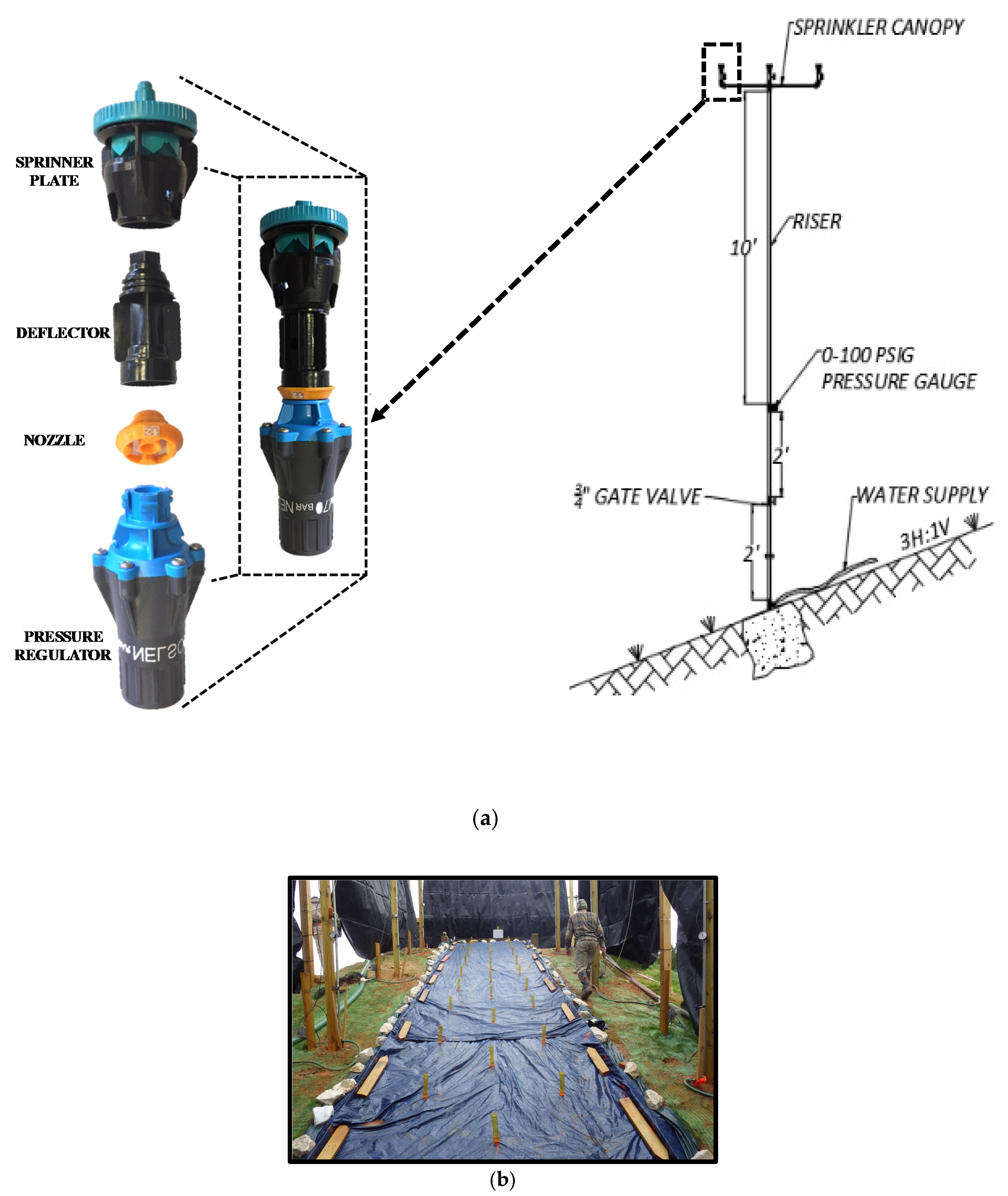
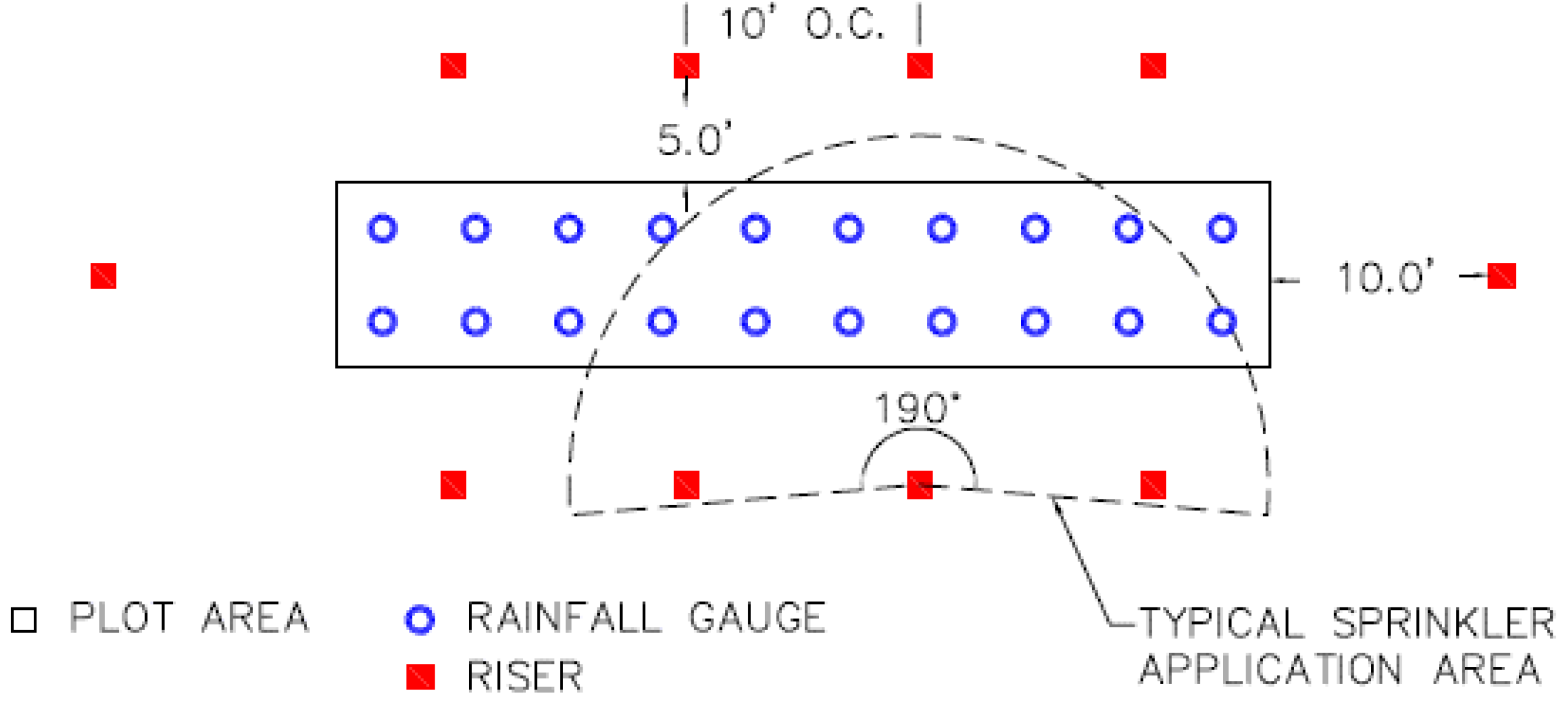
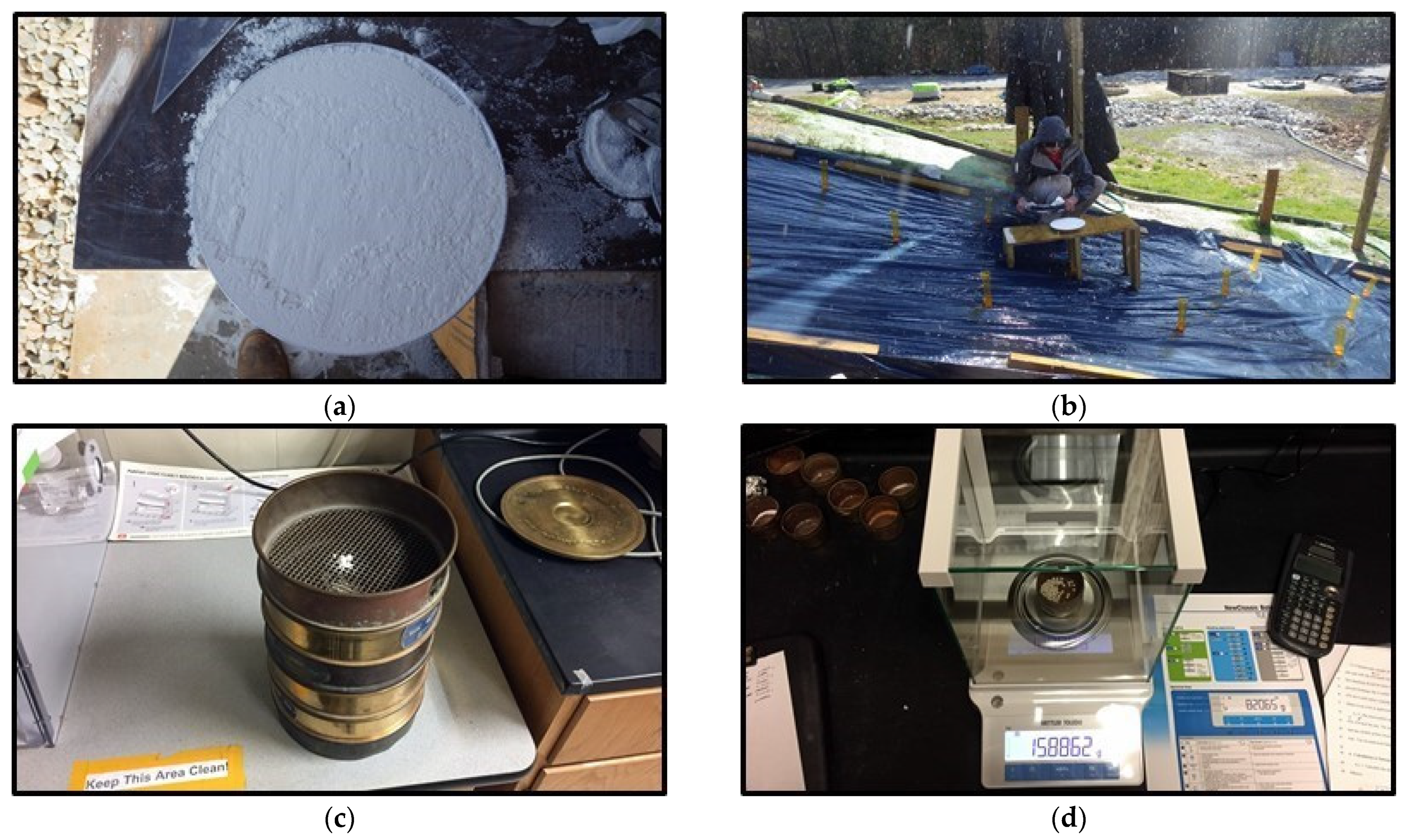
Following ASTM D6459-15, the rainfall simulator includes the use of sprinkler heads, sprinkler risers, pressure gauges, and valves. The ASTM design consists of nine sprinkler risers spaced evenly around the test plot. Raindrop sizes should vary from 1.0 to 6.0 mm (0.04 to 0.25 in.). Furthermore, the risers should be constructed to generate a minimum raindrop fall height of 4.3 m (14 ft). To conduct large-scale testing, a 12 m (40 ft) long by 2.4 m (8.0 ft) wide test plot must be constructed on a 3H:1V slope. The soil veneer used for testing should be placed in two, 15 cm (6.0 in.) lifts and must consist of either a loam, sand, or clay soil. The drop size distribution for a specific intensity is determined using the flour pan method [
24,
25]. Specified rainfall intensities are 50.8, 101.6, and 152.4 mm/hr (2.0, 4.0, and 6.0 in./hr). The test consists of three, 20-min intervals of increasing rainfall intensity for a total of 60 min.
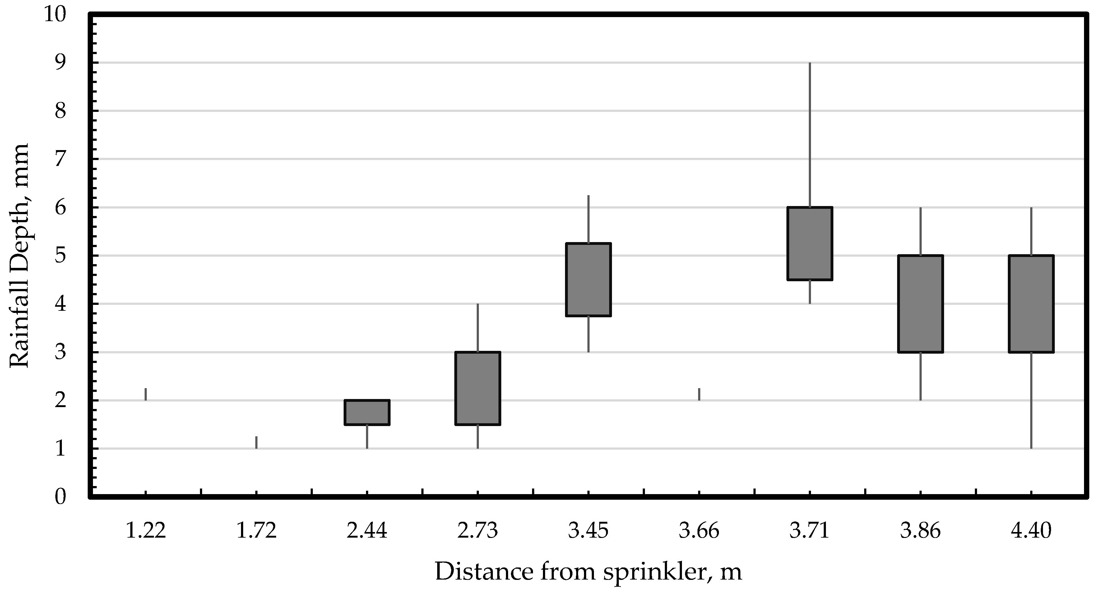
The ASTM standard requires apparatus calibration to ensure experimental values for uniformity of rainfall distribution, rainfall intensity, and drop size distribution are similar to natural rainfall. A calibration test consists of running the simulator at a specific intensity for 15 min. A collection of 20 rain gauges should be spaced throughout the test plot to collect rainfall data. The recorded rainfall depth in each rain gauge is analyzed to determine the experimental values for rainfall uniformity and intensity.
4. Results and Discussion
Calibration experiments were conducted to provide a means to quantify the performance of the rainfall simulator and determine if the apparatus is capable of simulating rainfall with characteristics similar to natural rainfall on a consistent basis. The methods and procedures previously discussed produced a multitude of data in the form of rainfall depth measured from each of the 29 rain gauges after each calibration test. The data from each test were analyzed to determine the average rainfall intensity and CUC. Finally, the values calculated from the calibration tests for each target rainfall intensity were averaged to provide a generalized report on the performance of the rainfall simulator in terms of experimental rainfall intensity and uniformity of rainfall distribution.
To validate the calibration process, a minimum of ten calibration tests for each intensity were conducted. If the standard deviation was less than or equal to 2.54 mm/hr (0.10 in./hr), testing efforts would proceed to the next interval. A maximum deviation of 2.54 mm/hr was set as the realistic limit for the simulator performing in a consistent and repeatable fashion. A total of 30, 15-min calibration tests were performed. The results from the calibration tests for all test intervals are summarized in
Table 3. The flow rate column represents the sum of the flow rates provided by the nozzles at a constant pressure of 41.4 kPa (6.0 psi).
After analyzing the values in
Table 3, it was concluded that the rainfall simulator consistently produced rainfall intensities slightly higher than the theoretical target. According to Meyer [
3] the experimental intensities should only vary from the theoretical intensities by a few percent. For the purpose of this study, the benchmark was set at 5.0%. Although the average rainfall intensities were higher than the theoretical target, the standard deviation between the 30 calibration tests was only 1.78 mm/hr (0.07 in./hr). This result ensured that the rainfall simulator was producing repeatable results in terms of rainfall intensity for all test intervals.
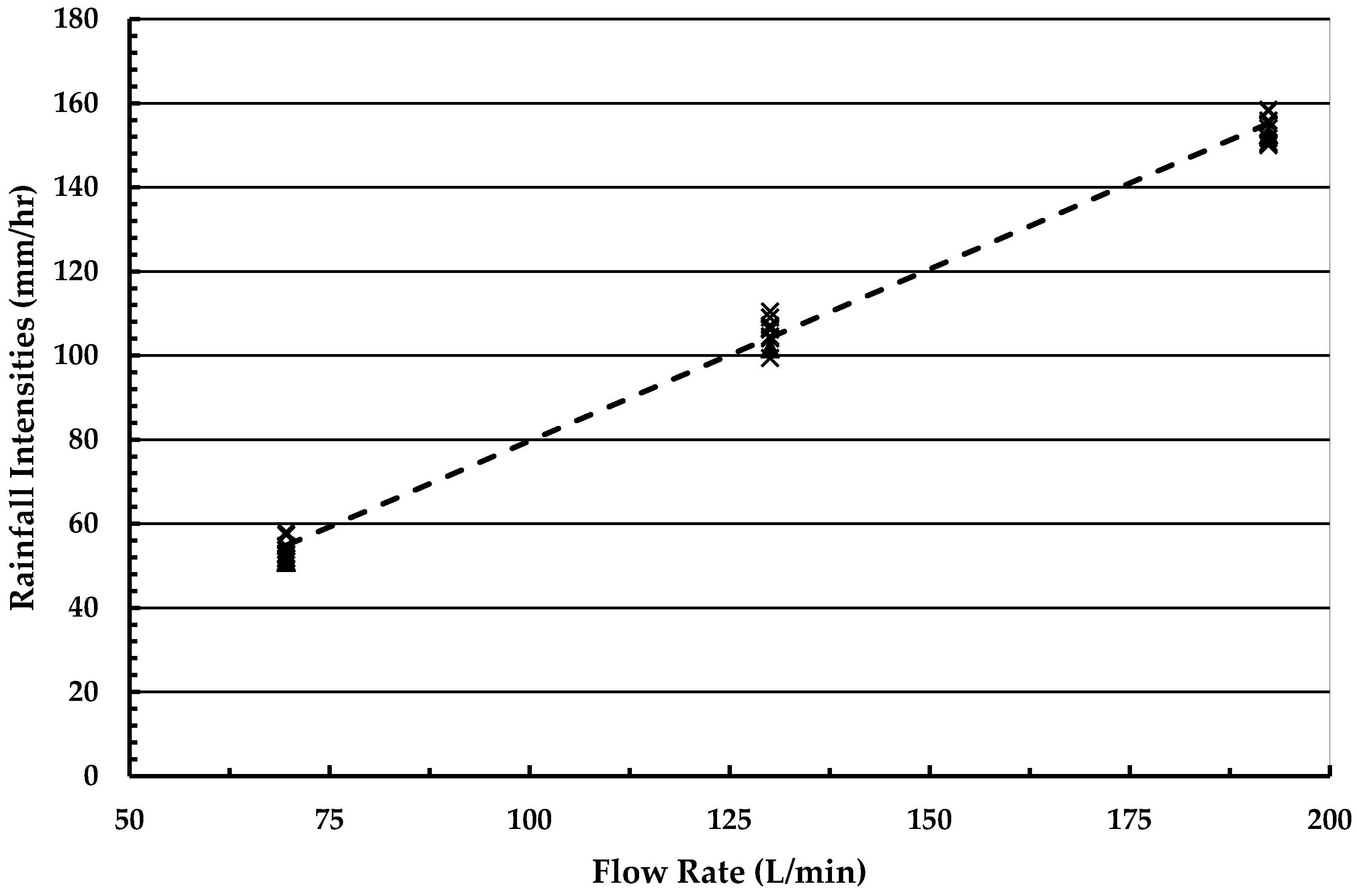
Figure 7 graphically illustrates that the experimental rainfall intensities calculated during calibration were typically slightly higher than the theoretical targets. The intensity produced by the rainfall simulator follows a linear pattern based on the total flow rate in the sprinkler heads. The
R2 value quantifies how accurately the trend line fits the data. With a
R2 value of 0.994, the linear trend line serves as a reliable means for estimating flow rates and corresponding nozzle sizes required to simulate specific rainfall intensities.
The average experimental rainfall intensities were used to calculate the
EI using Equation (6) and to compare against theoretical values.
EI is used in calculating the rainfall-runoff erosivity factor (R-factor) used in the RUSLE calculations for expected erosion over a given area. The R-factor is used to quantify the erosive energy of rainfall associated with specific storm events. The results from this analysis are presented in
Table 4.
The calculated values in
Table 4 correspond with the results from
Figure 6. The higher rainfall intensities produced by the rainfall simulator result in greater erosive potential on the test slope. The ensuing result is that higher rates of soil erosion are generated by the simulated rainfall versus what should be expected from the actual storm event. However, as the rainfall intensities increase, the relative error between the experimental and theoretical values decrease.
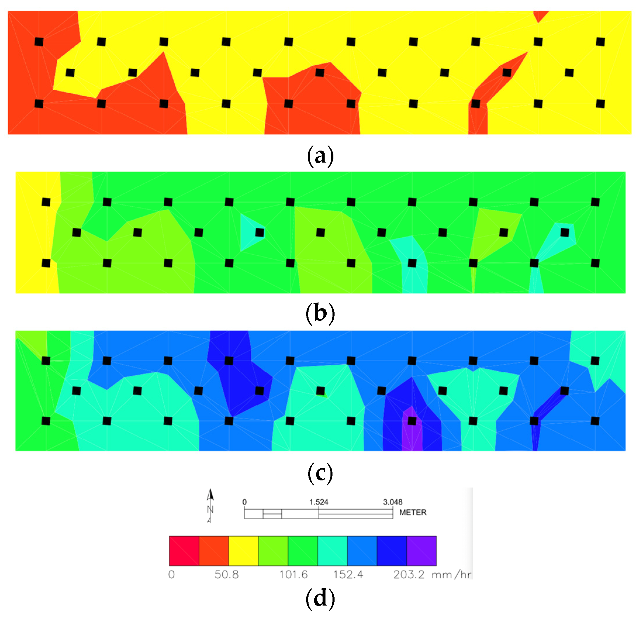
To aid in the visualization of the uniformity of rainfall distribution for each test interval, raster surfaces showing rainfall intensity were generated using AutoCAD Civil 3D
TM and overlaid on an aerial photo of the test plot as shown in
Figure 8. For each test interval, the rainfall intensities,
Figure 8a–c, were greatest in the middle of the test plot and lowest at the bottom of the test plot. The average uniformity of rainfall distribution for all tests performed ranged between 87.0 to 87.7%.
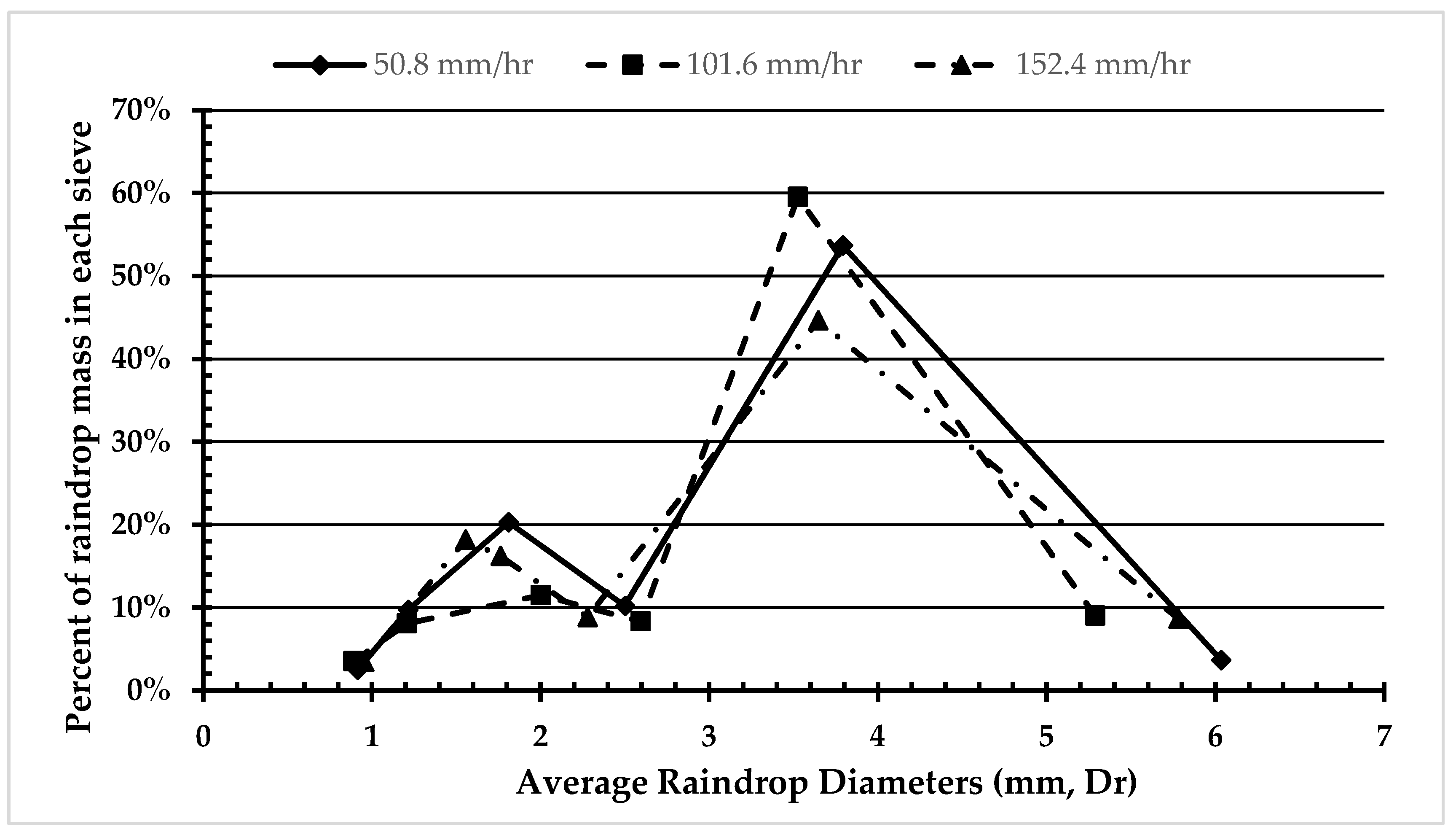
The rain drop diameters produced by the simulator were calculated using the flour pan method. The average drop diameter was then used to calculate the average mass of the rain drops (
Table 5). At each intensity, the calculated drop diameter was smaller than the theoretical value. Smaller diameter raindrops are produced when pressurized flow is discharged through small nozzle openings.
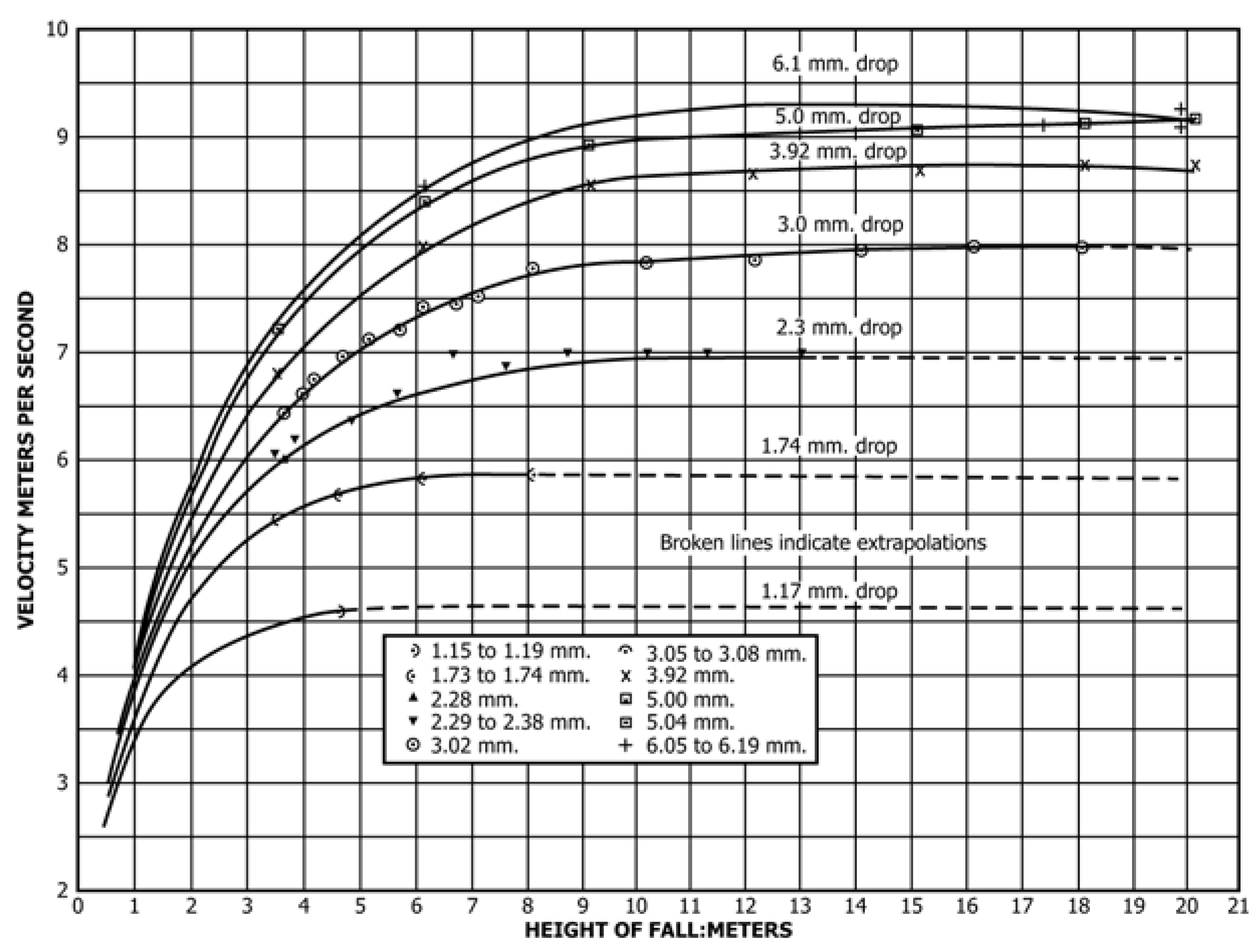
The values for average drop mass calculated previously were used to determine the experimental kinetic energy generated by the rainfall simulator (
Table 5). Values for rain drop velocity were estimated based on the diameter of the drop and the height from which the drops fell. In reality, the velocity of the drops is greater than estimated since the drops are projected from the sprinkler head with an initial outward and downward vector velocity. However, the actual velocities of raindrops were not quantified in this study.
As shown in
Table 5 above, the measured average drop diameter (D
50, in mm) for each interval was less than the theoretical drop diameters. However, the experimental drop diameters are consistent with other pressurized rainfall simulators as detailed in Bubenzer [
28]. As shown in Bubenzer [
28], the median drop diameter for pressured simulators ranged from 0.6 to 2.6 mm (0.02 to 0.10 in.), with the majority of the simulators producing a median drop diameter of 2.1 mm (0.08 in.).
For each rainfall intensity, the kinetic energy of a single raindrop is negligible. However, when combined with the energy of the thousands of other raindrops impacting the slope each second, the summation of this energy would be much more considerable.
4.1. Bare Soil Control Testing
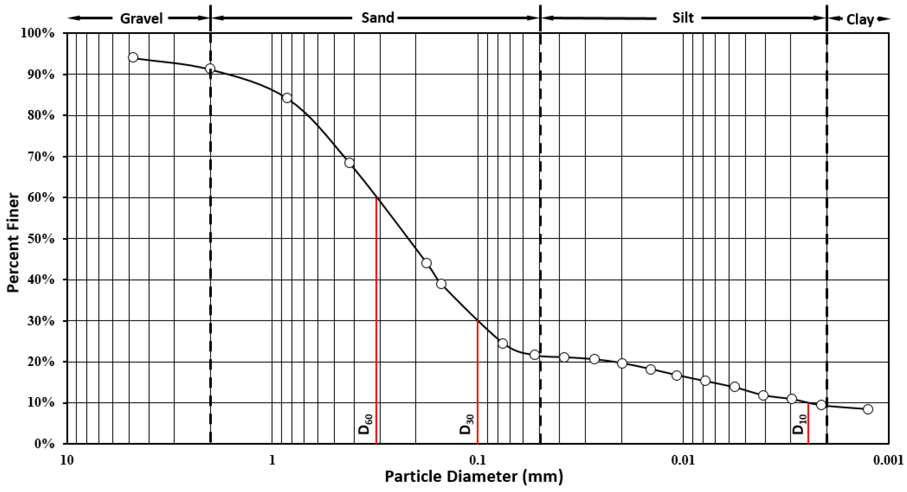
Once the rainfall simulator was calibrated, the next phase of the study involved performing a series of bare soil control tests for the design storm as specified in ASTM D6459-15. The tests consisted of a 60-min rainfall simulation with three separate intensities of 50.8, 101.6, and 152.4 mm/hr (2.0, 4.0, and 6.0 in/hr) for 20 min each. For these control tests, the soil tested was classified as a sandy loam as per the USDA soil texture triangle. The particle size distribution is shown below in
Figure 9.
Prior to performing each simulation, the test slope was prepared by tilling to a minimum depth of 10.2 cm (4.0 in.) and then compacting through the use of a lawn roller apparatus. The moisture content and compaction of the soil is then determined using the procedures outlined in ASTM D2937-10. During the simulation, grab samples of the runoff generated from the plot were captured at a maximum of every three minutes beginning once runoff began exiting the plot and continuing until the runoff ceased.
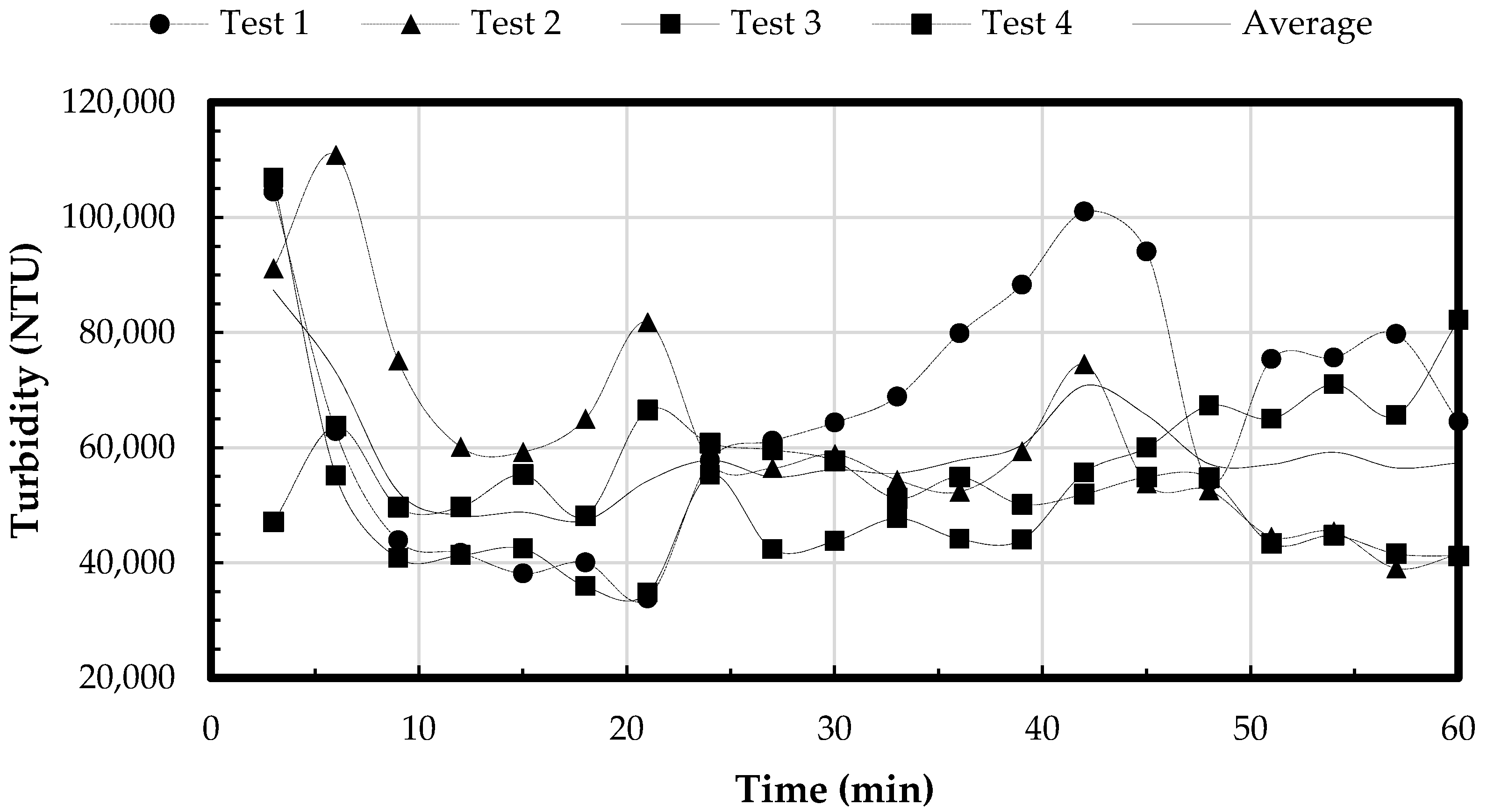
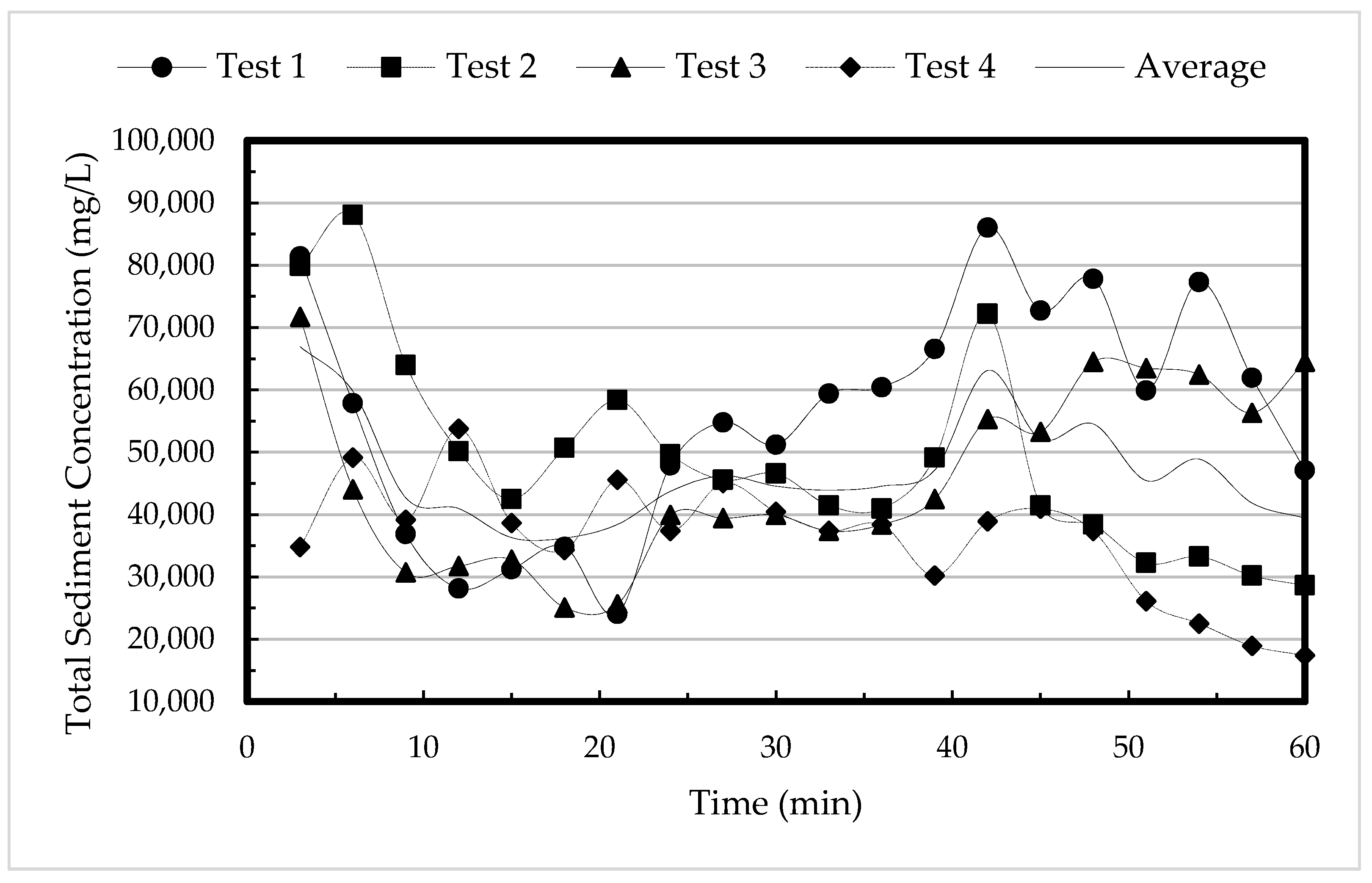
Summary plots are provided below in
Figure 10 and
Figure 11 for both turbidity and total sediment concentration, respectively, for the four bare soil control tests conducted. A summary of the results is shown below in
Table 6.
4.2. Use of the Erosion Index Equation for Simulated Rainfall
It should be considered that the erosion index described in Equation (4) was developed from analyzing soil erosion resulting from years of naturally occurring rainfall events. This results in an assumption of naturally occurring drop size distribution and the raindrops falling at terminal velocity. For predicting naturally occurring erosion rates based upon this Equation, these assumptions are relatively valid for in-field conditions. However, for synthetic rainfall produced by rainfall simulators, these conditions are difficult to create. For instance, based upon
Figure 6, a 3.0 mm (0.12 in.) raindrop has to fall approximately 16.0 m (52.5 ft) in a wind-free environment before reaching terminal velocity. ASTM D6459-15 only requires a minimum fall height of 4.26 m (14.0 ft). The nearest drop size plotted for this height in
Figure 6 is 1.17 mm (0.05 in.) drop diameter, which is smaller than the average drop size produced by most rainfall simulators used for erosion testing. This issue is addressed in ASTM D 6459-15, but only minimally. After calculating the erosion index using Equation (4), the standard specifies that the results of this calculation must then be corrected for the kinetic energy of the drops that are falling at less than terminal velocity. Since no further guidance in the standard is provided for correcting the results of Equation (4), it is left to the user to determine how to adjust.
However, adjusting the output of Equation (4) as the ASTM standard stipulates may not be necessary and potentially improper. It can be seen from this previous discussion that intensity is the correlative variable that helps define the energy of a naturally occurring storm event using Equations (3), (4), and (9). However, should “correcting Equation (4) for kinetic energy” be performed since the simulators are not producing naturally occurring rainfall energy? The point of using Equations (3), (4), and (9) is to bypass determining the kinetic energy of each storm directly by using intensity as a means of estimating energy. To be able to adjust EI from Equation (4), the kinetic energy from the simulated storm must be known. Therefore, since the storm is not naturally occurring and may not be adequately represented by Equation (4), it may be more prudent to simply use the kinetic energy calculations from Equation (9) and directly calculate EI30 using the simulator’s actual measured kinetic energy, instead of correcting Equation (4) that represents naturally occurring kinetic energy. These concepts require further evaluation and research, which is beyond the scope of this paper.
5. Summary and Conclusions
The purpose of this research study was to design and construct a large-scale rainfall simulator capable of repeatedly simulating rainfall with characteristics similar to natural rainfall. The design for the rainfall simulator was largely based on existing designs in ASTM D6459-15. However, changes were made due to the lack of specified products available for purchase and a desire to improve upon the existing ASTM standard testing method. Changes included: (1) using Nelson Irrigation PC-S3000 sprinkler heads in lieu of nozzles, no longer commercially available, stated in ASTM D6459-15) and (2) substituting solenoid valves in lieu of manual ball values. Discussion into the proper use of ASTM specified equations and their appropriateness were also introduced.
In accordance with ASTM D6459-15, rainfall intensities of 50.8, 101.6, 152.4 mm/hr (2.0, 4.0, and 6.0 in./hr) were simulated. Thirty, 15-min calibration experiments were conducted to determine the average experimental rainfall intensities and uniformities, drop size distribution, and erosive energy produced by the rainfall simulator. The experimental values were then compared with their corresponding theoretical targets to determine if the apparatus was adequately simulating natural rainfall. The theoretical target rainfall intensities for this study were 50.8, 101.6, and 152.4 mm/hr (2.0, 4.0, and 6.0 in./hr). The average experimental rainfall intensities produced by the rainfall simulator were found to be 53.8, 105.9, and 154.2 mm/hr (2.12, 4.17, and 6.07 in./hr), respectively. The uniformity of the rainfall distribution, quantified using CUC, was calculated to range between 87.0 to 87.7%. The corresponding average drop size were calculated to be 2.39, 2.58, and 2.35 mm (0.094, 0.101, and 0.093 in.), respectively. These results indicate that the rainfall simulator provides repeatable rainfall intensities, achieves uniformity, and produces consistent drop sizes.
As shown in
Figure 9 and
Figure 10 above, the simulator was also used to perform a series of bare soil control tests to establish a baseline for future evaluation of hillslope erosion control products. The results summarized in
Table 6 as well as the visual inspection of the test plot after each control test provide evidence that the rainfall simulator produced erosion results consistent within expected ranges. Visual inspections provided evidence of the occurrence of consistent splash erosion, sheet erosion, and rill erosion patterns; as well as consistent sediment yield, turbidity, and sediment concentrations measurements. Future research is also planned to test and evaluate various erosion control measures (i.e., rolled erosion control products, hydromulch, conventional mulching practices, etc.) on the test slope and to compare the performance and effectiveness of each respective practice in reducing erosion.


 ,
, 


