Identification of the Most Suitable Probability Distribution Models for Maximum, Minimum, and Mean Streamflow


Abstract
1. Introduction
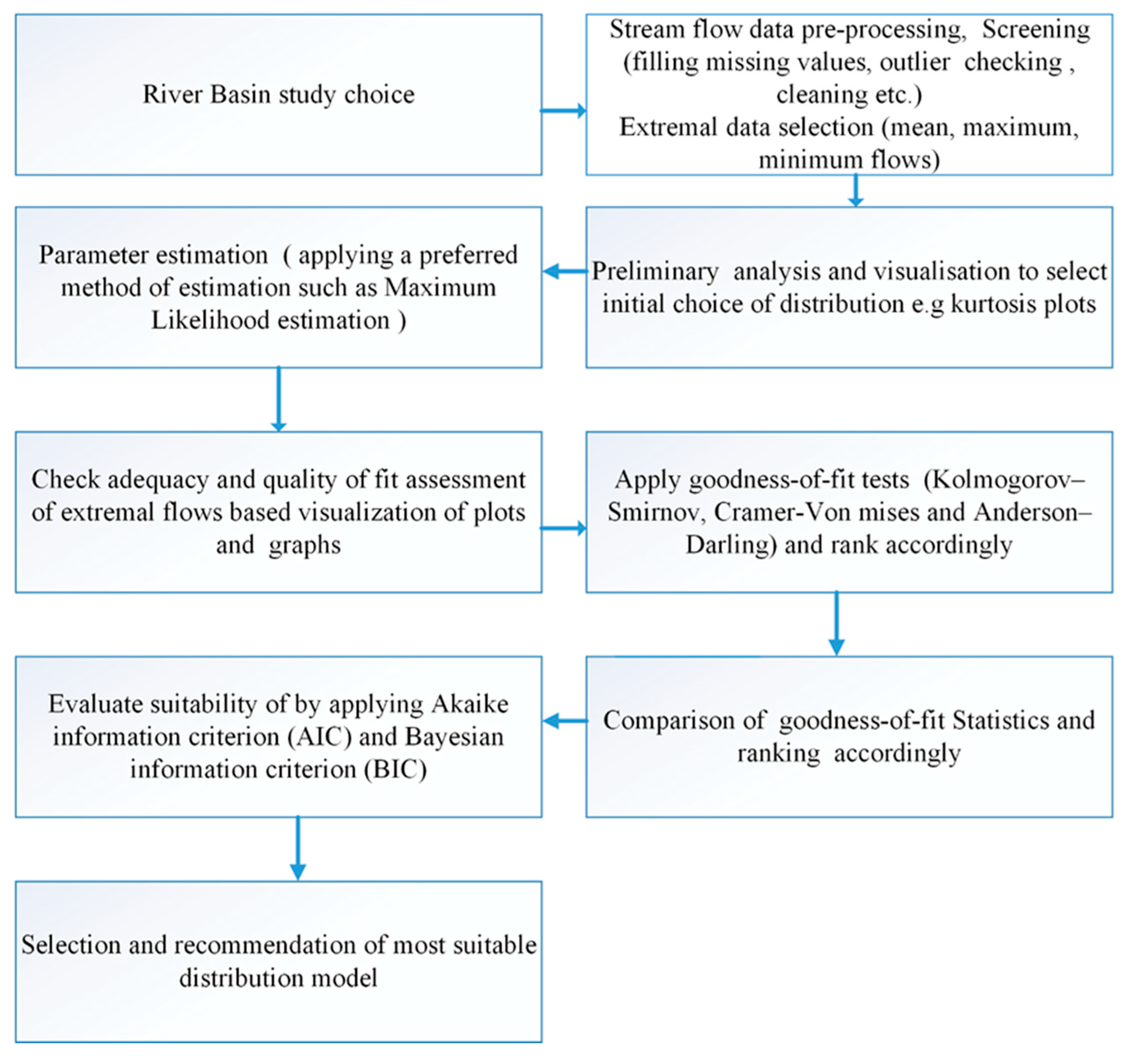
2. Basic Steps in the Identification of Probability Distribution Models
3. Study Site, Theoretical Descriptions, and Method
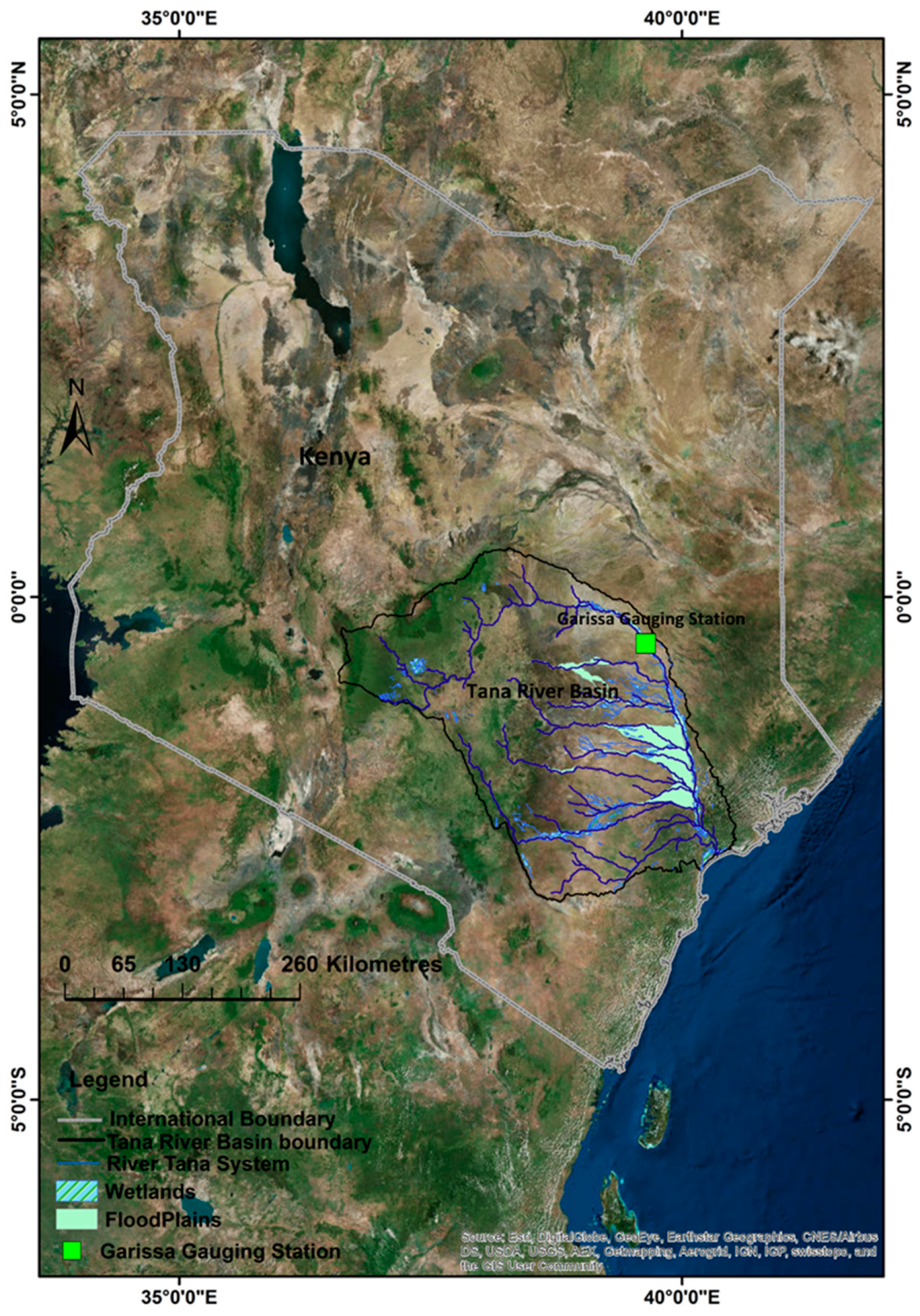
3.1. Study Site and Data
3.2. Maximum Likelihood Estimation Theory
3.3. Goodness of Fit (GoF) Test
3.4. Anderson–Darling (AD) Test
3.5. Kolmogorov–Smirnov Test
3.6. Cramer–Von Mises Test
3.7. Method
4. Results
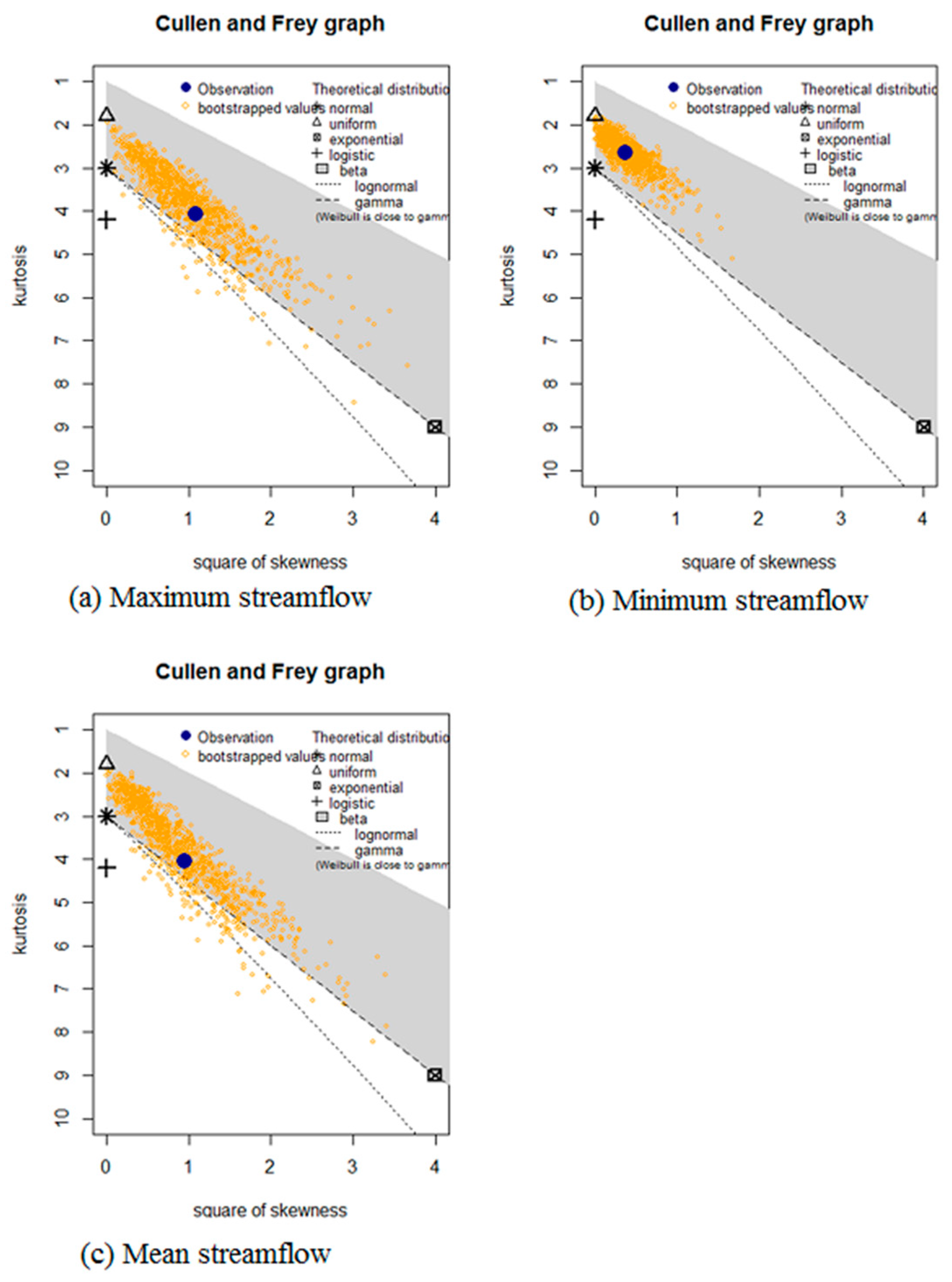
4.1. Preliminary Assessment and Visualisation
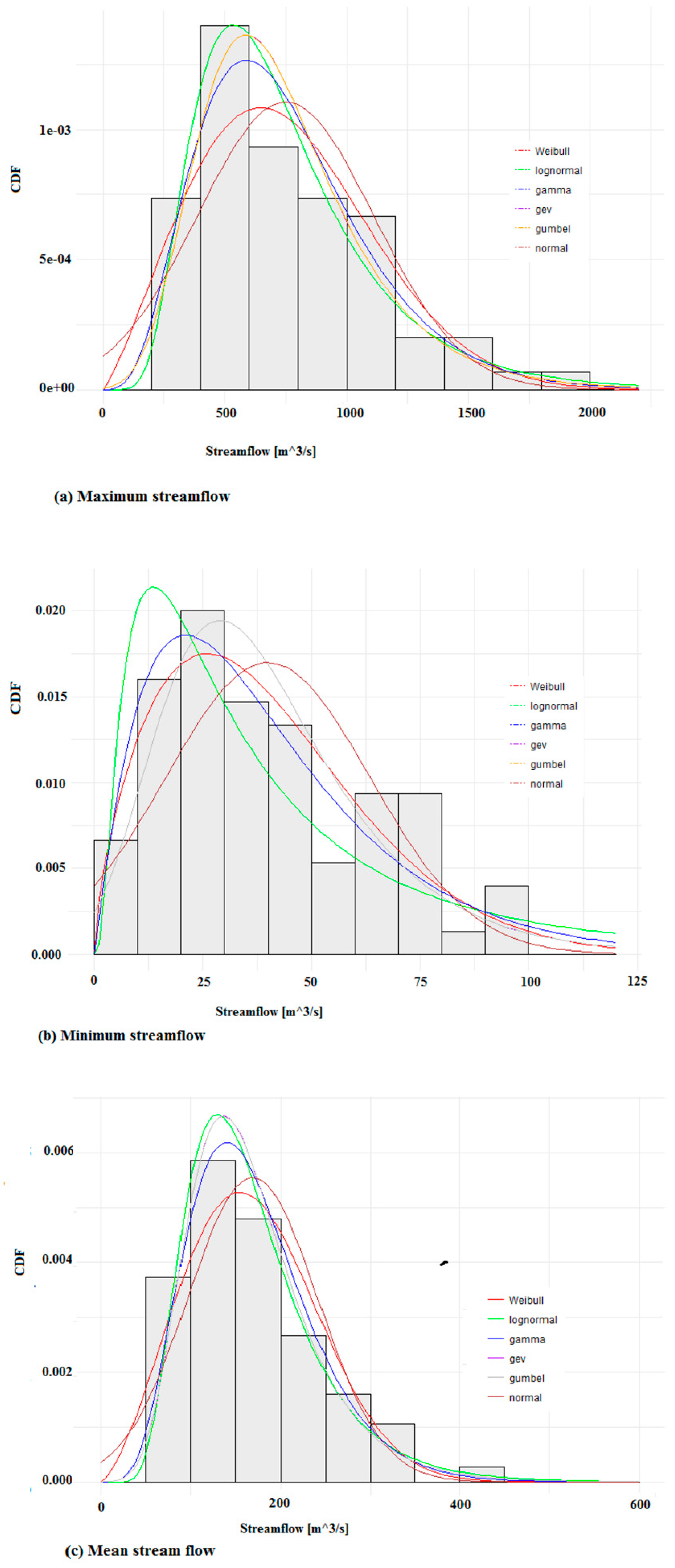
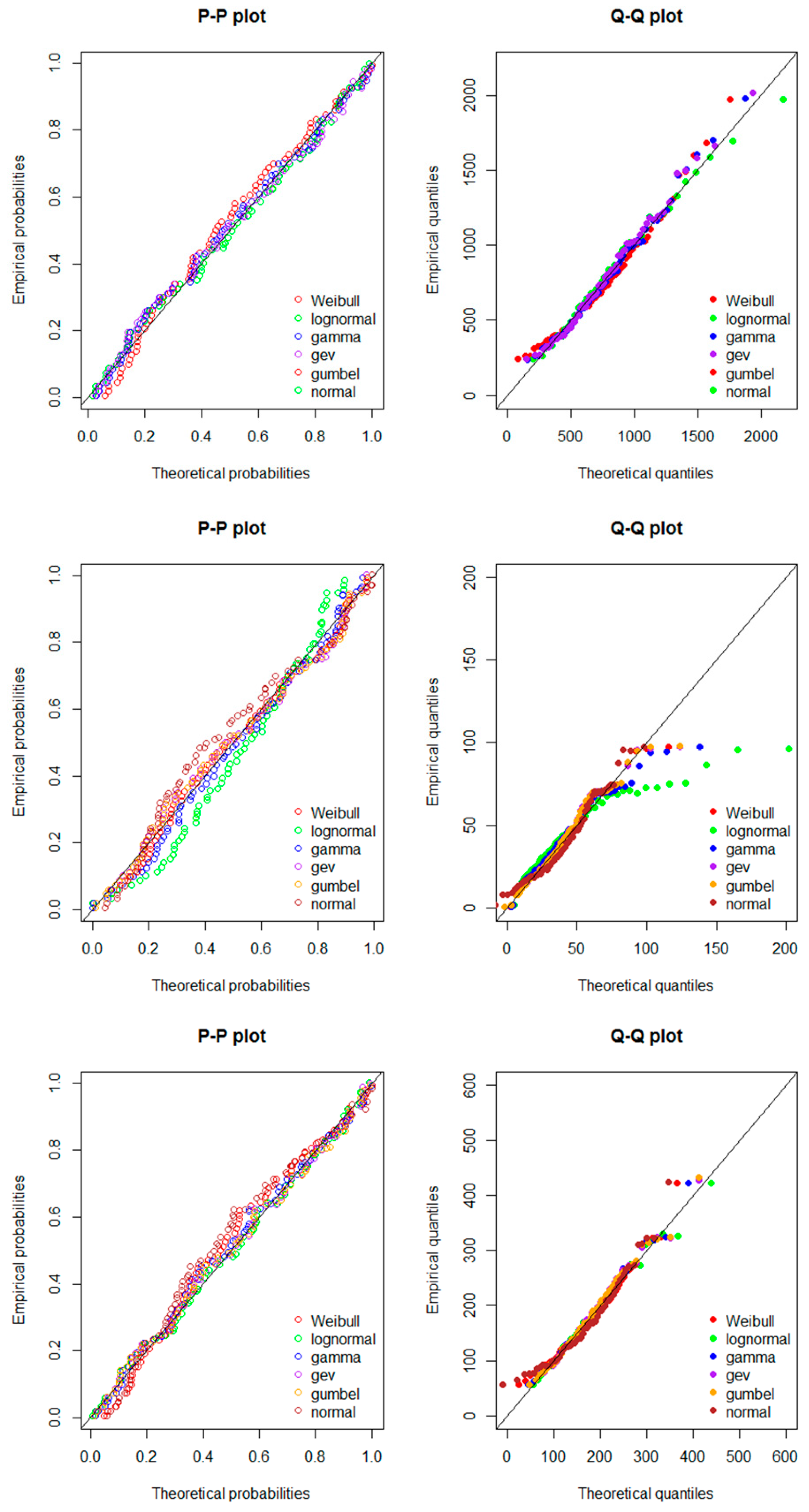
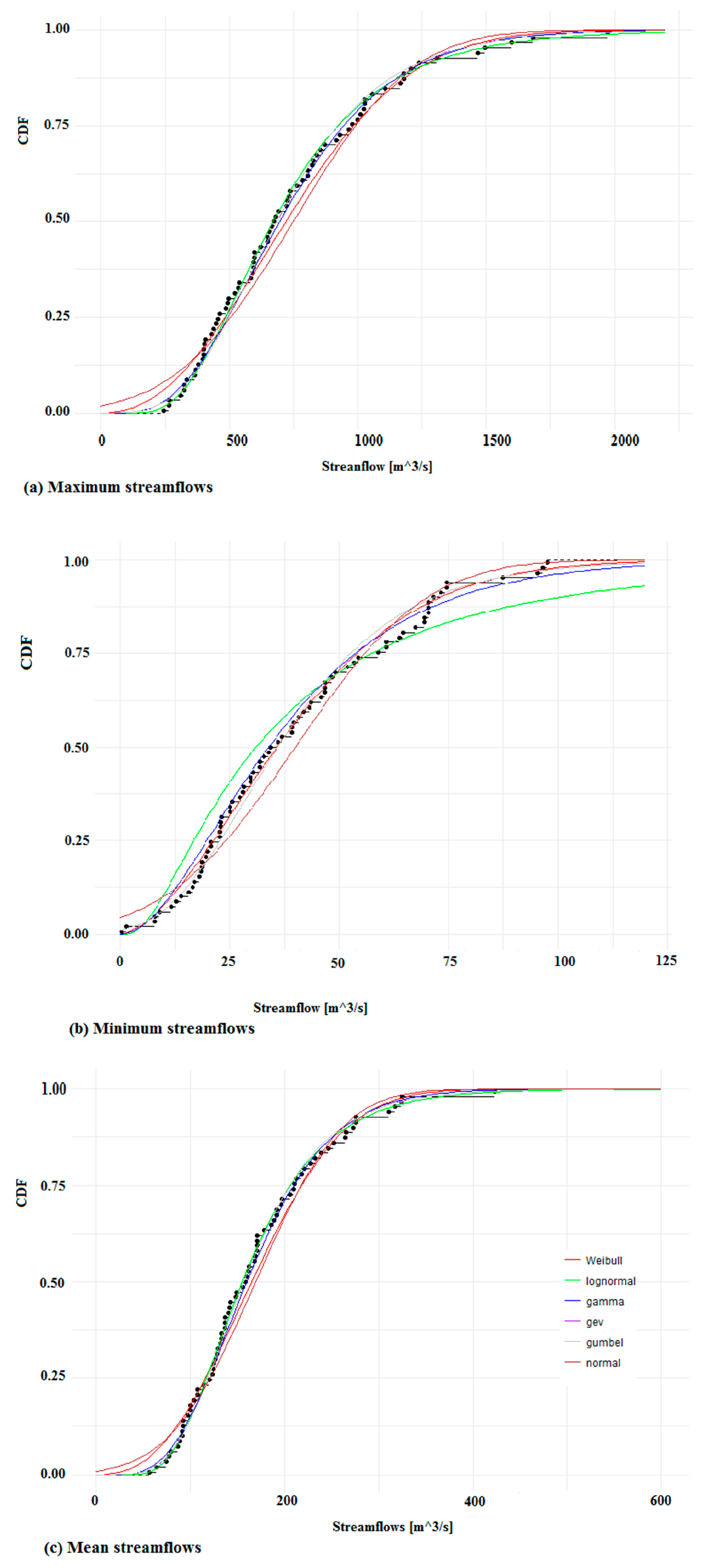
4.2. Goodness of Fit Using Assessment-Based Graphs
4.3. GoF Test-Based Analysis
4.4. Best-Fit Distribution Model
5. Discussion
6. Conclusions
- a.
- Gamma (Pearson type 3) and lognormal distribution models were selected as the best-fit functions for maximum streamflows. The Weibull, GEV, and Gumbel functions were the best-fit functions for the Tana River annual minimum flows, while the lognormal and GEV distribution functions were the best-fit functions for the Tana River annual mean flows. The models may be used in forecasting hydrologic events, detecting the inherent stochastic characteristics of hydrologic variables, filling missing data of observations in proximal areas, and extending records for predictions and water engineering purposes.
- b.
- The GoF tests-based analysis and procedures are useful in the selection of suitable distribution model functions for the site
- c.
- Different distribution functions may be suitable for the minimum, mean, and maximum flood frequency estimations at the same site; therefore, the choice of a suitable model for flood frequency analysis at a site with the same climatic, catchment, and hydrological characteristics depends on the frequency regime of the data series.
Author Contributions
Acknowledgments
Conflicts of Interest
References
- Myronidis, D.; Stathis, D.; Sapountzis, M. Post-Evaluation of Flood Hazards Induced by Former Artificial Interventions along a Coastal Mediterranean Settlement. J. Hydrol. Eng. 2016, 21, 05016022. [Google Scholar] [CrossRef]
- Smith, J.A.; Baeck, M.L.; Villarini, G.; Wright, D.B.; Krajewski, W. Extreme flood response: The June 2008 flooding in Iowa. J. Hydrometeorol. 2013, 14, 1810–1825. [Google Scholar] [CrossRef]
- Tegos, A.; Schlüter, W.; Gibbons, N.; Katselis, Y.; Efstratiadis, A. Assessment of Environmental Flows from Complexity to Parsimony—Lessons from Lesotho. Water 2018, 10, 1293. [Google Scholar] [CrossRef]
- Srikanthan, R.; Amirthanathan, G.; Kuczera, G. Real-time flood forecasting using ensemble kalman filter. In MODSIM 2007 International Congress on Modelling and Simulation; Modelling and Simulation Society of Australia and New Zealand: Christchurch, New Zealand, 2007; pp. 1789–1795. [Google Scholar]
- Bolaji, G.; Agbede, O.; Adewumi, J.; Akinyemi, J. Selection of flood frequency model in niger basin using maximum likelihood method. In Water and Urban Development Paradigms: Towards an Integration of Engineering, Design and Management Approaches; Taylor & Francis: Abingdon, UK, 2008; p. 337. [Google Scholar]
- Cunnane, C. Statistical distributions for flood frequency analysis. In Operational Hydrology Report (WMO); WMO: Geneva, Switzerland, 1989. [Google Scholar]
- Myronidis, D.; Ioannou, K. Forecasting the urban expansion effects on the design storm hydrograph and sediment yield using artificial neural networks. Water 2019, 11, 31. [Google Scholar] [CrossRef]
- Flynn, K.M.; Kirby, W.H.; Hummel, P.R. User’s Manual for Program Peakfq, Annual Flood-Frequency Analysis Using Bulletin 17b Guidelines; U.S. Geological Survey: Reston, VA, USA, 2006; pp. 2328–7055.
- Hill, P.; Graszkiewicz, Z.; Sih, K.; Nathan, R.; Loveridge, M.; Rahman, A. Outcomes from a pilot study on modelling losses for design flood estimation. In Proceedings of the Hydrology and Water Resources Symposium 2012, Sydney, Australia, 19–22 November 2012; p. 1449. [Google Scholar]
- Loveridge, M.; Rahman, A. Probabilistic losses for design flood estimation: A case study in new south wales. In Proceedings of the Hydrology and Water Resources Symposium 2012, Sydney, Australia, 19–22 Noveber 2012; p. 9. [Google Scholar]
- Helsel, D.R.; Hirsch, R.M. Statistical Methods in Water Resources; US Geological Survey: Reston, VA, USA, 2002; Volume 323. [Google Scholar]
- Ndetei, C.; Opere, A.; Mutua, F. Flood frequency analysis in lake victoria basin based on tail behaviour of distributions. J. Kenya Meteorol. Soc. 2007, 1, 44–54. [Google Scholar]
- Khosravi, G.; Majidi, A.; Nohegar, A. Determination of suitable probability distribution for annual mean and peak discharges estimation (case study: Minab river-barantin gage, iran). Int. J. Probab. Stat. 2012, 1, 160–163. [Google Scholar] [CrossRef][Green Version]
- Bobee, B.; Cavadias, G.; Ashkar, F.; Bernier, J.; Rasmussen, P. Towards a systematic approach to comparing distributions used in flood frequency analysis. J. Hydrol. 1993, 142, 121–136. [Google Scholar] [CrossRef]
- Serinaldi, F.; Kilsby, C.G.; Lombardo, F. Untenable nonstationarity: An assessment of the fitness for purpose of trend tests in hydrology. Adv. Water Resour. 2018, 111, 132–155. [Google Scholar] [CrossRef]
- Thomas, W.O., Jr. A uniform technique for flood frequency analysis. J. Water Resour. Plan. Manag. 1985, 111, 321–337. [Google Scholar] [CrossRef]
- Stedinger, J.R.; Griffis, V.W. Flood Frequency Analysis in the United States: Time to Update; American Society of Civil Engineers: Reston, VA, USA, 2008. [Google Scholar]
- Koskinas, A.; Tegos, A.; Tsira, P.; Dimitriadis, P.; Iliopoulou, T.; Papanicolaou, P.; Koutsoyiannis, D.; Williamson, T. Insights into the oroville dam 2017 spillway incident. Geosciences 2019, 9, 37. [Google Scholar]
- Olofintoye, O.; Sule, B.; Salami, A. Best–fit probability distribution model for peak daily rainfall of selected cities in nigeria. N. Y. Sci. J. 2009, 2, 1–12. [Google Scholar]
- Engeland, K.; Hisdal, H.; Frigessi, A. Practical extreme value modelling of hydrological floods and droughts: A case study. Extremes 2004, 7, 5–30. [Google Scholar] [CrossRef]
- Potter, K.W.; Lettenmaier, D.P. A comparison of regional flood frequency estimation methods using a resampling method. Water Resour. Res. 1990, 26, 415–424. [Google Scholar] [CrossRef]
- Hosking, J.R. L-moments: Analysis and estimation of distributions using linear combinations of order statistics. J. R. Stat. Soc. Ser. B (Methodol.) 1990, 105–124. [Google Scholar] [CrossRef]
- Vogel, R.M.; McMahon, T.A.; Chiew, F.H. Floodflow frequency model selection in australia. J. Hydrol. 1993, 146, 421–449. [Google Scholar] [CrossRef]
- Hoskins, J.; Wallis, J. Regional Frequency Analysis: An Approach Based on L-Moments; Cambridge University: Cambridge, UK, 1997. [Google Scholar]
- Kysely, J.; Picek, J. Regional growth curves and improved design value estimates of extreme precipitation events in the czech republic. Clim. Res. 2007, 33, 243–255. [Google Scholar] [CrossRef]
- Elamir, E.A.; Seheult, A.H. Trimmed l-moments. Comput. Stat. Data Anal. 2003, 43, 299–314. [Google Scholar] [CrossRef]
- Wang, Q.J. Lh moments for statistical analysis of extreme events. Water Resour. Res. 1997, 33, 2841–2848. [Google Scholar] [CrossRef]
- Nouri Gheidari, M.H. Comparisons of the l-and lh-moments in the selection of the best distribution for regional flood frequency analysis in lake urmia basin. Civ. Eng. Environ. Syst. 2013, 30, 72–84. [Google Scholar] [CrossRef]
- Cohn, T.; Lane, W.; Baier, W. An algorithm for computing moments-based flood quantile estimates when historical flood information is available. Water Resour. Res. 1997, 33, 2089–2096. [Google Scholar] [CrossRef]
- Griffis, V.; Stedinger, J.; Cohn, T. Log pearson type 3 quantile estimators with regional skew information and low outlier adjustments. Water Resour. Res. 2004, 40. [Google Scholar] [CrossRef]
- Greenwood, J.A.; Landwehr, J.M.; Matalas, N.C.; Wallis, J.R. Probability weighted moments: Definition and relation to parameters of several distributions expressable in inverse form. Water Resour. Res. 1979, 15, 1049–1054. [Google Scholar] [CrossRef]
- Kuczera, G. Comprehensive at-site flood frequency analysis using monte carlo bayesian inference. Water Resour. Res. 1999, 35, 1551–1557. [Google Scholar] [CrossRef]
- Ribatet, M.; Sauquet, E.; Grésillon, J.-M.; Ouarda, T.B.M.J. A regional bayesian pot model for flood frequency analysis. Stoch. Environ. Res. Risk Assess. 2007, 21, 327–339. [Google Scholar] [CrossRef]
- Ouarda, T.; El-Adlouni, S. Bayesian nonstationary frequency analysis of hydrological variables 1. J. Am. Water Resour. Assoc. 2011, 47, 496–505. [Google Scholar] [CrossRef]
- Wang, X.; Zhou, J.; Zhang, L. The probability density evolution method for flood frequency analysis: A case study of the nen river in china. Water 2015, 7, 5134–5151. [Google Scholar] [CrossRef]
- Strupczewski, W.; Singh, V.; Feluch, W. Non-stationary approach to at-site flood frequency modelling i. Maximum likelihood estimation. J. Hydrol. 2001, 248, 123–142. [Google Scholar] [CrossRef]
- Jin, M.; Stedinger, J.R. Flood frequency analysis with regional and historical information. Water Resour. Res. 1989, 25, 925–936. [Google Scholar] [CrossRef]
- Martins, E.S.; Stedinger, J.R. Generalized maximum-likelihood generalized extreme-value quantile estimators for hydrologic data. Water Resour. Res. 2000, 36, 737–744. [Google Scholar] [CrossRef]
- Hosking, J.R. Moments or l moments? An example comparing two measures of distributional shape. Am. Stat. 1992, 46, 186–189. [Google Scholar] [CrossRef]
- Madsen, H.; Pearson, C.P.; Rosbjerg, D. Comparison of annual maximum series and partial duration series methods for modeling extreme hydrologic events: 2. Regional modeling. Water Resour. Res. 1997, 33, 759–769. [Google Scholar] [CrossRef]
- Laio, F.; Di Baldassarre, G.; Montanari, A. Model selection techniques for the frequency analysis of hydrological extremes. Water Resour. Res. 2009, 45. [Google Scholar] [CrossRef]
- Haddad, K.; Rahman, A. Selection of the best fit flood frequency distribution and parameter estimation procedure: A case study for tasmania in australia. Stoch. Environ. Res. Risk Assess. 2011, 25, 415–428. [Google Scholar] [CrossRef]
- Griffis, V.; Stedinger, J. Log-pearson type 3 distribution and its application in flood frequency analysis. I: Distribution characteristics. J. Hydrol. Eng. 2007, 12, 482–491. [Google Scholar] [CrossRef]
- Rahman, A.S.; Rahman, A.; Zaman, M.A.; Haddad, K.; Ahsan, A.; Imteaz, M. A study on selection of probability distributions for at-site flood frequency analysis in australia. Natural Hazards 2013, 69, 1803–1813. [Google Scholar] [CrossRef]
- Vogel, R.M.; Thomas, W.O., Jr.; McMahon, T.A. Flood-flow frequency model selection in southwestern united states. J. Water Resour. Plan. Manag. 1993, 119, 353–366. [Google Scholar] [CrossRef]
- Langat, P.K.; Kumar, L.; Koech, R. Understanding water and land use within tana and athi river basins in kenya: Opportunities for improvement. Sustain. Water Resour. Manag. 2018, 1–11. [Google Scholar] [CrossRef]
- van Beukering, P.; de Moel, H.; Botzen, W.; Eiselin, M.; Kamau, P.; Lange, K.; van Maanen, E.; Mogol, S.; Mulwa, R.; Otieno, P. The economics of ecosystem services of the tana river basin-assessment of the impact of large infrastructural interventions. R-Report 2015, 15, 3. [Google Scholar]
- Saji, N.; Goswami, B.; Vinayachandran, P.; Yamagata, T. A dipole mode in the tropical indian ocean. Nature 1999, 401, 360. [Google Scholar] [CrossRef]
- Birkett, C.; Murtugudde, R.; Allan, T. Indian ocean climate event brings floods to east africa’s lakes and the sudd marsh. Geophys. Res. Lett. 1999, 26, 1031–1034. [Google Scholar] [CrossRef]
- Koei, N. The Project on the Development of the National Water Master Plan 2030; Final Report; Volume v Sectoral Report (e)—Agriculture and Irrigation; the Republic of Kenya; Water Resources Management Authority: Nairobi, Kenya, 2013.
- Langat, P.K.; Kumar, L.; Koech, R. Temporal variability and trends of rainfall and streamflow in tana river basin, kenya. Sustainability 2017, 9, 1963. [Google Scholar] [CrossRef]
- Seckin, N.; Yurtal, R.; Haktanir, T.; Dogan, A. Comparison of probability weighted moments and maximum likelihood methods used in flood frequency analysis for ceyhan river basin. Arab. J. Sci. Eng. 2010, 35, 49. [Google Scholar]
- Ojha, C.; Berndtsson, R.; Bhunya, P.A. Books published. Environ. Manag. 2009, 1, 117–131. [Google Scholar]
- Rao, A.; Hamed, K. The logistic distribution. In Flood Frequency Analysis; CRC Press: Boca Raton, FL, USA, 2000; pp. 291–321. [Google Scholar]
- Zhang, J. Powerful goodness-of-fit tests based on the likelihood ratio. J. R. Stat.Soc. Ser. B (Stat. Methodol.) 2002, 64, 281–294. [Google Scholar] [CrossRef]
- Anderson, T.W.; Darling, D.A. Asymptotic theory of certain” goodness of fit” criteria based on stochastic processes. Ann. Math. Stat. 1952, 23, 193–212. [Google Scholar] [CrossRef]
- Chakravarti, I.M.; Laha, R.G.; Roy, J. Handbook of Methods of Applied Statistics; Wiley Series in Probability and Mathematical Statistics (USA) eng; Wiley: Hoboken, NJ, USA, 1967. [Google Scholar]
- Stephens, M.A. Tests based on edf statistics. In Goodness-of-Fit Techniques; d’agostino, R.B., Stephens, M.A., Eds.; Marcel Dekker: New York, NY, USA, 1986; pp. 1–15. [Google Scholar]
- Cullen, A.C.; Frey, H.C.; Frey, C.H. Probabilistic Techniques in Exposure Assessment: A Handbook for Dealing with Variability and Uncertainty in Models and Inputs; Springer Science & Business Media: New York, NY, USA, 1999. [Google Scholar]
- D’Agostino, R.B.; Stephens, M.A. Goodness-fo-Fit-Techniques; Taylor & Francis: Abingdon, UK, 1986. [Google Scholar]
- Akaike, H. Information theory and an extension of the maximum likelihood principle. In Selected Papers of Hirotugu Akaike; Springer: Berlin/Heidelberg, Germany, 1998; pp. 199–213. [Google Scholar]
- Raftery, A.E. Bayesian model selection in social research. Sociol. Methodol. 1995, 25, 111–163. [Google Scholar] [CrossRef]
- Dewan, A.; Corner, R.; Saleem, A.; Rahman, M.M.; Haider, M.R.; Rahman, M.M.; Sarker, M.H. Assessing channel changes of the ganges-padma river system in bangladesh using landsat and hydrological data. Geomorphology 2017, 276, 257–279. [Google Scholar] [CrossRef]
- Ihaka, R.; Gentleman, R. R: A language for data analysis and graphics. J. Comput. Graph. Stat. 1996, 5, 299–314. [Google Scholar]
- Zambrano-Bigiarini, M. Package ‘hydroTSM: Time Series Management, Analyis and Interpolation for Hydrological Modelling. 2017. Available online: https://cran.r-project.org/package=hydroTSM (accessed on 25 October 2017).
- Cisty, M.; Celar, L. Using r in water resources education. Int. J. Innov. Educ. Res. 2015, 3, 97–117. [Google Scholar]
- Delignette-Muller, M.L.; Dutang, C.; Pouillot, R.; Denis, J.-B.; Siberchicot, A.; Siberchicot, M.A. Package ‘fitdistrplus’. R Foundation for Statistical Computing, Vienna, Austria. 2017. Available online: http://www. R-project. org (accessed on 25 October 2017).
- Babu, G.J.; Rao, C. Goodness-of-fit tests when parameters are estimated. Sankhya 2004, 66, 63–74. [Google Scholar]
- Volpi, E.; Fiori, A.; Grimaldi, S.; Lombardo, F.; Koutsoyiannis, D. Save hydrological observations! Return period estimation without data decimation. J. Hydrol. 2019, 571, 782–792. [Google Scholar] [CrossRef]
- Blom, G. Statistical Estimates and Transformed Beta Variables; Wiley: New York, NY, USA, 1958. [Google Scholar]
- Thyer, M.; Renard, B.; Kavetski, D.; Kuczera, G.; Franks, S.W.; Srikanthan, S. Critical evaluation of parameter consistency and predictive uncertainty in hydrological modeling: A case study using bayesian total error analysis. Water Resour. Res. 2009, 45. [Google Scholar] [CrossRef]
- Beard, L.R. Book review: The gamma family and derived distributions applied in hydrology. By bernard bobee and fahim ashkar, water resources publications, littleton, co 80161-2841, USA, 1991, 203 pp., soft cover, $38.00, isbn 0-918334-68-3. J. Hydrol. 1992, 132, 383. [Google Scholar] [CrossRef]
- Guru, N.; Jha, R. Flood frequency analysis of tel basin of mahanadi river system, india using annual maximum and pot flood data. Aquat. Procedia 2015, 4, 427–434. [Google Scholar] [CrossRef]
- Vogel, R.M.; Wilson, I. Probability distribution of annual maximum, mean, and minimum streamflows in the united states. J. Hydrol. Eng. 1996, 1, 69–76. [Google Scholar] [CrossRef]
- Survey, G.; Speer, P.R.; Golden, H.G. Low-Flow Characteristics of Streams in the Mississippi Embayment in Mississippi and Alabama; US Government Printing Office: Washington, DC, USA, 1964.
- Agwata, J.F. Water resources utilization, conflicts and interventions in the tana basin of Kenya. FWU Water Resour. Publ. 2005, 3, 13–23. [Google Scholar]
- Eris, E.; Aksoy, H.; Onoz, B.; Cetin, M.; Yuce, M.I.; Selek, B.; Aksu, H.; Burgan, H.I.; Esit, M.; Yildirim, I. Frequency analysis of low flows in intermittent and non-intermittent rivers from hydrological basins in turkey. Water Sci. Technol. Water Supp. 2019, 19, 30–39. [Google Scholar] [CrossRef]
- Laio, F. Cramer–von mises and anderson-darling goodness of fit tests for extreme value distributions with unknown parameters. Water Resour. Res. 2004, 40. [Google Scholar] [CrossRef]
- Blum, A.G.; Archfield, S.A.; Vogel, R.M. On the probability distribution of daily streamflow in the united states. Hydrol. Earth Syst. Sci. 2017, 21, 3093–3103. [Google Scholar] [CrossRef]
- Dimitriadis, P.; Koutsoyiannis, D. Stochastic synthesis approximating any process dependence and distribution. Stoch. Environ. Res. Risk Assess. 2018, 32, 1493–1515. [Google Scholar] [CrossRef]
- Dimitriadis, P.; Koutsoyiannis, D. Climacogram versus autocovariance and power spectrum in stochastic modelling for markovian and hurst–kolmogorov processes. Stoch. Environ. Res. Risk Assess. 2015, 29, 1649–1669. [Google Scholar] [CrossRef]
- Koutsoyiannis, D. Statistics of extremes and estimation of extreme rainfall: I. Theoretical investigation/statistiques de valeurs extrêmes et estimation de précipitations extrêmes: I. Recherche théorique. Hydrol. Sci. J. 2004, 49. [Google Scholar] [CrossRef]
- Dimitriadis, P.; Tegos, A.; Oikonomou, A.; Pagana, V.; Koukouvinos, A.; Mamassis, N.; Koutsoyiannis, D.; Efstratiadis, A. Comparative evaluation of 1d and quasi-2d hydraulic models based on benchmark and real-world applications for uncertainty assessment in flood mapping. J. Hydrol. 2016, 534, 478–492. [Google Scholar] [CrossRef]
- Ngongondo, C.; Li, L.; Gong, L.; Xu, C.-Y.; Alemaw, B.F. Flood frequency under changing climate in the upper kafue river basin, southern africa: A large scale hydrological model application. Stoch. Environ. Res. Risk Assess. 2013, 27, 1883–1898. [Google Scholar] [CrossRef]
- Koutsoyiannis, D. Generic and parsimonious stochastic modelling for hydrology and beyond. Hydrol. Sci. J. 2016, 61, 225–244. [Google Scholar] [CrossRef]


| Distribution Model | Probability Distribution Function (PDF) | Range |
|---|---|---|
| Gamma (Pearson type 3) | Q ≥ 0, α, β > 0 | |
| Lognormal | < Q < | |
| Weibull | ||
| GEV | Q > for | |
| Gumbel | ||
| Normal |
| Statistic | Extreme Streamflow Datasets | ||
|---|---|---|---|
| Maximum Streamflow | Minimum Streamflow | Mean Streamflow | |
| Minimum (m3/s) | 244.89 | 0.22 | 56.73 |
| Maximum (m3/s) | 1974.02 | 97.61 | 423.04 |
| Median (m3/s) | 674.05 | 34.37 | 157.93 |
| Mean (m3/s) | 749.22 | 39.98 | 169.21 |
| Estimated standard deviation (m3/s) | 363.10 | 23.65 | 72.29 |
| Estimated skewness | 1.04 | 0.62 | 0.98 |
| Estimated kurtosis | 4.063 | 2.645 | 4.048 |
| Maximum Flows | Minimum Flows | Mean Flows | |||||||||||
|---|---|---|---|---|---|---|---|---|---|---|---|---|---|
| Distribution | Standard Error | Correlation Matrix | Standard Error | Correlation Matrix | Standard Error | Correlation Matrix | |||||||
| Sample estimate | Standard Error | Shape | Scale | Sample Estimate | Standard Error | Shape | Scale | Sample estimate | Standard Error | Shape | Scale | ||
| Gamma (Pearson type 3) | shape | 4.65 | 0.64 | 1.00 | 0.93 | 2.11 | 0.32 | 1.00 | 0.89 | 5.92 | 0.93 | 1.00 | 0.96 |
| scale | 0.01 | 0.00 | 0.93 | 1.00 | 0.05 | 0.01 | 0.89 | 1.00 | 0.03 | 0.01 | 0.96 | 1.00 | |
| Lognormal | shape | 6.51 | 0.48 | 1.00 | 0.00 | 3.43 | 0.11 | 0.00 | 1.00 | 5.04 | 0.05 | 1.00 | 0.00 |
| scale | 0.05 | 0.04 | 0.00 | 1.00 | 0.91 | 0.07 | 1.00 | 0.00 | 0.42 | 0.03 | 0.00 | 1.00 | |
| Weibull | shape | 2.22 | 0.19 | 1.00 | 0.33 | 1.68 | 0.16 | 1.00 | 0.30 | 2.50 | 0.05 | 1.00 | 0.00 |
| scale | 849.40 | 46.93 | 0.33 | 1.00 | 44.49 | 3.20 | 0.30 | 1.00 | 0.42 | 0.03 | 0.00 | 1.00 | |
| GEV | shape | 587.02 | 32.71 | 1.00 | 0.31 | 28.99 | 2.30 | 1.00 | 0.32 | 136.67 | 6.70 | 1.00 | 0.31 |
| scale | 269.54 | 25.18 | 0.31 | 1.00 | 18.92 | 1.73 | 0.32 | 1.00 | 55.12 | 5.08 | 0.31 | 1.00 | |
| Gumbel | shape | 587.07 | 32.72 | 1.00 | 0.31 | 28.99 | 2.30 | 1.00 | 0.32 | 136.66 | 6.70 | 1.00 | 0.31 |
| scale | 269.62 | 25.20 | 0.31 | 1.00 | 18.92 | 1.73 | 0.32 | 1.00 | 55.17 | 5.09 | 0.31 | 1.00 | |
| Normal | shape | 749.22 | 41.65 | 1.00 | 0.00 | 39.98 | 2.71 | 1.00 | 0.00 | 169.21 | 8.29 | 1.00 | 0.00 |
| scale | 360.66 | 29.45 | 0.00 | 1.00 | 23.49 | 1.92 | 0.00 | 1.00 | 71.81 | 5.86 | 0.00 | 1.00 | |
| Distribution | Kolmogorov–Smirnov (Critical Value at 0.05 = 0.20517) | Cramer–von Mises (Critical Value at 0.05 = 0.221) | Anderson–Darling (Critical Value at 0.05 = 2.5018) | |||
|---|---|---|---|---|---|---|
| Statistic | Rank | Statistic | Rank | Statistic | Rank | |
| Maximum Streamflow | ||||||
| Gamma (Pearson type 3) | 0.0568 | 2 | 0.0377 | 2 | 0.2771 | 2 |
| Lognormal | 0.0545 | 1 | 0.0307 | 1 | 0.2048 | 1 |
| Weibull | 0.0705 | 5 | 0.0845 | 5 | 0.6521 | 5 |
| GEV | 0.0635 | 3 | 0.0452 | 3 | 0.3294 | 3 |
| Gumbel | 0.0692 | 4 | 0.0633 | 4 | 0.4271 | 4 |
| Normal | 0.1011 | 6 | 0.2088 | 6 | 1.2463 | 6 |
| Minimum Streamflow | ||||||
| Gamma (Pearson type 3) | 0.0711 | 4 | 0.0668 | 4 | 0.6331 | 4 |
| Lognormal | 0.1296 | 6 | 0.3389 | 6 | 2.4926 | 6 |
| Weibull | 0.0549 | 1 | 0.0411 | 1 | 0.4007 | 1 |
| GEV | 0.0693 | 2 | 0.0633 | 2 | 0.4272 | 3 |
| Gumbel | 0.0693 | 2 | 0.0633 | 2 | 0.4271 | 2 |
| Normal | 0.1011 | 5 | 0.2088 | 5 | 1.2463 | 5 |
| Mean Streamflow | ||||||
| Gamma (Pearson type 3) | 0.0621 | 4 | 0.0349 | 4 | 0.2341 | 4 |
| Lognormal | 0.0410 | 1 | 0.0193 | 1 | 0.1425 | 1 |
| Weibull | 0.0956 | 5 | 0.1068 | 5 | 0.7245 | 5 |
| GEV | 0.0455 | 3 | 0.0269 | 3 | 0.1988 | 3 |
| Gumbel | 0.0453 | 2 | 0.0267 | 2 | 0.1972 | 2 |
| Normal | 0.1168 | 6 | 0.1883 | 6 | 1.1685 | 6 |
| Distribution | Maximum Streamflow | Minimum Streamflow | Mean Streamflow | |||
|---|---|---|---|---|---|---|
| AIC | BIC | AIC | BIC | AIC | BIC | |
| Gamma (Pearson type 3) | 1083.1 | 1087.7 | 687.3 | 691.9 | 844.4 | 849.0 |
| Lognormal | 1081.4 | 1086.0 | 718.0 | 722.7 | 843.2 | 847.8 |
| Weibull | 1089.5 | 1094.1 | 682.1 | 686.8 | 851.5 | 856.2 |
| GEV | 1083.7 | 1088.4 | 682.2 | 686.8 | 844.1 | 848.7 |
| Gumbel | 1083.7 | 1088.4 | 682.2 | 686.8 | 844.1 | 857.9 |
| Normal | 1100.0 | 1104.7 | 690.3 | 694.9 | 848.7 | 862.6 |
© 2019 by the authors. Licensee MDPI, Basel, Switzerland. This article is an open access article distributed under the terms and conditions of the Creative Commons Attribution (CC BY) license (http://creativecommons.org/licenses/by/4.0/).
Share and Cite
Langat, P.K.; Kumar, L.; Koech, R. Identification of the Most Suitable Probability Distribution Models for Maximum, Minimum, and Mean Streamflow. Water 2019, 11, 734. https://doi.org/10.3390/w11040734
Langat PK, Kumar L, Koech R. Identification of the Most Suitable Probability Distribution Models for Maximum, Minimum, and Mean Streamflow. Water. 2019; 11(4):734. https://doi.org/10.3390/w11040734
Chicago/Turabian StyleLangat, Philip Kibet, Lalit Kumar, and Richard Koech. 2019. "Identification of the Most Suitable Probability Distribution Models for Maximum, Minimum, and Mean Streamflow" Water 11, no. 4: 734. https://doi.org/10.3390/w11040734
APA StyleLangat, P. K., Kumar, L., & Koech, R. (2019). Identification of the Most Suitable Probability Distribution Models for Maximum, Minimum, and Mean Streamflow. Water, 11(4), 734. https://doi.org/10.3390/w11040734