1. Introduction
In the past decade, there has been an increasing use of dual-drainage models, linking storm water pipe flow (the buried system or minor system) to the overland flow (the major system). Models of the minor system increasingly allow for detailed modelling of the network through representing all manholes, combined sewer overflows, outlet devices, control facilities, among others, usually by defining discharge coefficients [
1,
2]. On the other hand, some particular structures and devices, such as gullies and manholes, have been analyzed using either experimental investigation [
3,
4] or computational fluid dynamics (
) [
2] in order to understand flows and search for parameters that characterize such flows. The understanding of the underlying physics and the capability to model these physical phenomena allowing to adequately predict the flow field is of paramount importance to perform numerical environmental studies [
5]. This detail has not been extended effectively to the interface devices between the overland drainage system and the buried drainage infrastructure, although it is well known that flooding can be caused or aggravated by insufficient flow capacity of the inlet devices [
6,
7,
8]. The hydraulic capacity of gullies has been related with factors such as the flow depth on the surface, surface flow conditions, grate type and clogging conditions, inlet area and dimensions, geometry and slope of streets and gullies [
8,
9,
10,
11]. Factors such as the local geometry and the location of the gully outlet are also known to influence the flow.
is becoming increasingly used as part of simulation schemes for hydraulic structures in urban drainage systems [
2,
11,
12,
13]. In particular, Beg et al. [
2] tested different turbulence models and compared them with experimental measurements, concluding that Shear Stress Transport (
)
k-
and Renormalization Group (
)
k-
turbulence models reached best accuracy. Also Lopes et al. [
13] presented simulations of a specific gully using
-
with a high accuracy.
Different gully geometries may be found throughout the world. It seems that their geometry and details follow some regional traditional criteria and that sometimes they are constrained by the street and sewer system location.
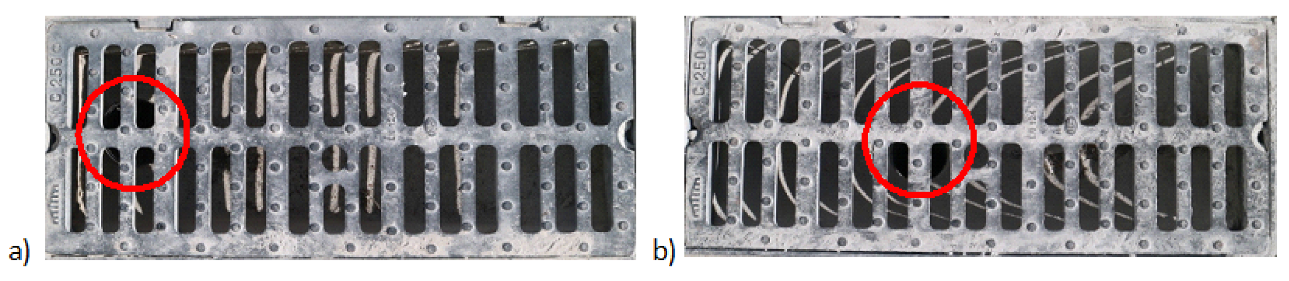
Figure 1 illustrates two gullies, where the connections to the buried system are vertical and located in two different positions along the gully longitudinal axis. The inlet efficiency of gullies is not well known, and their discharge coefficients depend mainly on the geometry, the hydraulic head, and the velocity field [
14]. In that work, the authors found that the initial conditions have a great influence in the time to attain steady conditions. They concluded that the outlet position can influence discharge coefficients. This work aims to study the hydraulic behavior of gullies in usual drainage conditions featuring different locations of the vertical outlet pipe that connects the gully to the buried drainage system, taking into consideration different outlet dimensions, as well as a large range of discharge flows, and 2D and 3D analyses.
The
model constructed using
code was validated in [
10,
11,
15,
16], and [
13] by comparing with experimental measurements. Different gully models for different outlet locations and dimensions were now constructed and those were used to simulate a wide range of discharge flows. We present the qualitative description of the gully flow in steady and unsteady conditions as well as the quantitative analysis of the following parameters along the gully: water depths, streamlines, velocity, pressure fields, and the inlet discharge capacity.
2. Numerical Model
The numerical model is based on the Navier–Stokes equations/Reynolds-Averaged Navier–Stokes (
) equations governing the motion of the
incompressible and isothermal flows in which the free surface is described using a Volume-Of-Fluid method (
). According to this description [
17,
18], the
-function,
, ranging from 0 to 1 and corresponding respectively to cells without water and full occupied by water, is included in the mass and momentum conservation equations. It is also updated using an advection equation for
F. Some improvements of
models were developed including surface tension and the interface curvature, as well as the artificial compression of the interface, to improve accuracy of the interface [
19]. The
method used in the interFoam solver implemented in the
(Equations (
1)–(
3)) has two particularities: a volumetric surface force, explicitly estimated by the Continuum Surface Force (
) function of the surface tension, and the interface curvature, which are included in the momentum equation [
20]; the compression of the interface is achieved by introducing an extra, artificial compression term in the advection equation [
19,
21].
where
is the mean velocity vector,
is the modified pressure adapted by removing the hydrostatic pressure from the total pressure,
is the
F function,
t is the time,
is the fluid density,
is the acceleration due to gravity,
is the shear stress tensor,
is the volumetric surface tension force (where
and interface curvature are included) and
is the compression velocity.
Further in the mass and momentum conservation equations,
-function is included through physical properties such as density and viscosity, which are defined by a weighting of the values for air and water. Lopes et al. [
13] developed an air-entrainment model. The new solver, airInterFoam, considers the air entrainment triggered by an additional advection equation for dispersed gas phase. Lopes et al. [
13] thus simulated a gully with air and water flow, led to conclusion on whether to consider the air-entrainment or not. Although important air-entrainment occurs, it revealed small influence on the hydraulic performance of the gully. They also used a turbulence model, where turbulence variables were calculated with the
-
turbulence model. This is known for the best combination of two Reynolds-Averaged Simulation (
) formulations, using high-Reynolds-number formulation of k-
model for the free-stream region and taking advantage of the accuracy and robustness of
k-
model in the near-wall zone. This study follows the Lopes et al. [
13] methodology. However, the air-entrainment model was not used as it is not needed for the detailed requirements, saving computer time.
Total Variation Diminishing (
) limited form of central-differencing is used for convective terms in momentum equation. The Van-Leer scheme is used for the convective term in
-advection equation and ‘Interface Compression’ scheme is used in order to bound the solution of the compressive term between 0 and 1. To ensure boundedness of the phase fraction and avoid interface smearing, the solution of the
equation is done with the Multidimensional Universal Limiter for Explicit Solutions (
). The Pressure-Implicit with Splitting of Operators (
) procedure proposed by [
22] is used for pressure velocity coupling in transient calculations with 3 loops. We used the same discretization schemes employed in previous works on gullies tested with positive outcome [
10,
13] as well as we used turbulence models with the best accuracy [
2].
The computational domain of the flow, aiming to represent a length (L) × width × height = m × m × m gully placed in a 1% sloped piece of the street pavement, was defined by a box m long ( m m), m wide ( m m) and m high ( m m), using a grid of cells with variable spacing ( m minimum).
The gully was placed between
m and
m of the street (
m
m). The mesh analysis was done and presented in [
13]. We tested three meshes. The two finer meshes showed equivalent vortex details, therefore we choose an intermediate mesh size, which retains the main features of the vortices, while also keeping the calculation time acceptable. We constructed the
geometry using blockMesh utility from
adapting the work of [
10,
13].
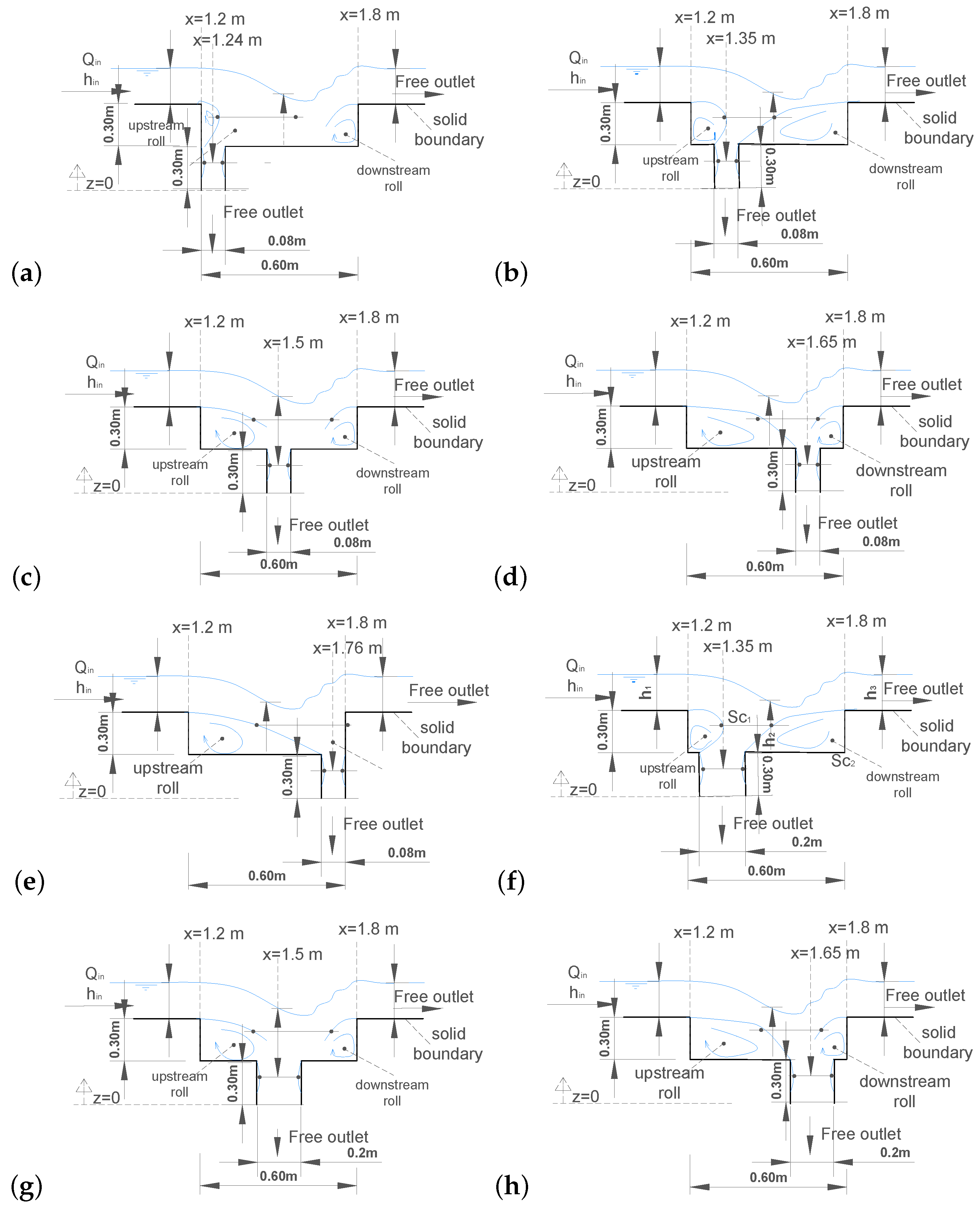
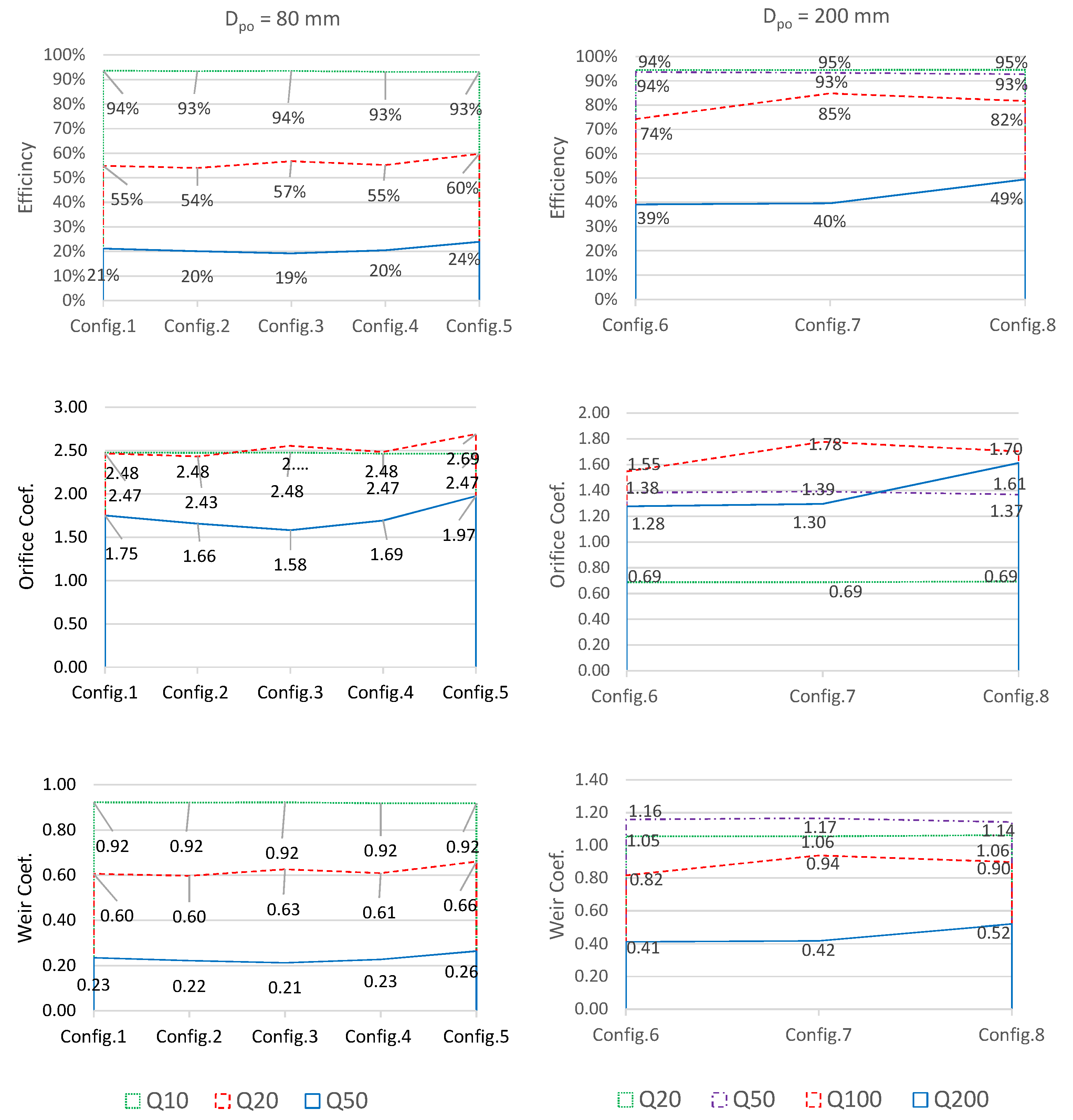
Figure 2 presents the longitudinal cross sections of the eight gully configurations studied indicating the outlet vertical pipe position center (
). We consider five configurations for an outlet pipe of diameter
= 80 mm (Configurations 1 to 5, which corresponds to five different locations from upstream to downstream) and three configurations for an outlet pipe of diameter
= 200 mm (Configurations 6 to 8, which corresponds to three different locations from upstream to downstream).
Table 1 summarizes the outlet pipe characteristics for each configuration.
To simplify the mesh construction, we considered xx-axis parallel to the channel bottom instead of it being horizontal. Thus, the acceleration due to gravity, instead of being considered vertical, was set to to consider a 1% slope. The different configurations of the gully outlet were simulated for different flow rates (3 discharges for Config. 1 to 5: Q10, Q20, and Q50) and 4 discharges for Config.6 to 8: Q20, Q50, Q100, and Q200).
The upstream inflow boundary condition (BC) defined as Dirichlet-BC, at
0, was set according to supercritical uniform conditions in a hypothetical
m wide channel and 1% slope street.
Table 2 presents the inflow conditions for the different discharge flows in supercritical uniform conditions, supercritical uniform height,
, and uniform velocity,
, which was considered constant along the depth, as well as Froude and Reynolds numbers (
,
, with
being the viscosity).
The inlet and outlet at the right boundary (downstream channel) were defined by a specific gradient for dynamic part of pressure (). In the outlet at the bottom (outlet pipe) a hydrostatic pressure was assumed. The top boundary considered hydrostatic pressure and specific gradient for VOF and velocity. The remain boundaries were considered as walls, imposing zero velocity in the vicinity of the face using Dirichlet-BC.


 .
.


