Intelligent Control/Operational Strategies in WWTPs through an Integrated Q-Learning Algorithm with ASM2d-Guided Reward

Abstract

The operation of a wastewater treatment plant (WWTP) is a typical complex control problem, with nonlinear dynamics and coupling effects among the variables, which renders the implementation of real-time optimal control an enormous challenge. In this study, a Q-learning algorithm with activated sludge model No. 2d-guided (ASM2d-guided) reward setting (an integrated ASM2d-QL algorithm) is proposed, and the widely applied anaerobic-anoxic-oxic (AAO) system is chosen as the research paradigm. The integrated ASM2d-QL algorithms equipped with a self-learning mechanism are derived for optimizing the control strategies (hydraulic retention time (HRT) and internal recycling ratio (IRR)) of the AAO system. To optimize the control strategies of the AAO system under varying influent loads, Q matrixes were built for both HRTs and IRR optimization through the pair of <max reward-action> based on the integrated ASM2d-QL algorithm. 8 days of actual influent qualities of a certain municipal AAO wastewater treatment plant in June were arbitrarily chosen as the influent concentrations for model verification. Good agreement between the values of the model simulations and experimental results indicated that this proposed integrated ASM2d-QL algorithm performed properly and successfully realized intelligent modeling and stable optimal control strategies under fluctuating influent loads during wastewater treatment.

1. Introduction

Wastewater treatment plants (WWTPs), recognized as the fundamental tools for municipal and industrial wastewater treatment, are the crucial urban infrastructures to improve the water environment [1]. However, today, the performance of the existing WWTPs worldwide is facing more and more severe challenges [2,3,4]. For instance, in China, the existing WWTPs are confronted with considerable non-standard wastewater discharge and serious abnormal operation issues [5]. By the end of 2013, 3508 WWTPs had been built in 31 provinces in China; however, almost 90% of them have inescapable problems with nutrient removal, and roughly ⁓50% of WWTPs could not meet the nitrogen discharge standard [6]. Since the quality of the discharged effluent is one of the most serious environmental problems today, the ever increasingly stringent standards and regulations for the operation of WWTPs have been imposed by authorities and legislation [7,8]. Therefore, the implementation of effluent standards requires refined and sophisticated control strategies able to deal with this nonlinear and multivariable system with complex dynamics [9,10].

The task of optimizing wastewater treatment process is highly challenging since the optimal operating conditions of the WWTP are difficult to be controlled due to its biological, physical, and chemical processes are complex, interrelated, and highly nonlinear [11]. Increasing attention to modeling wastewater processes has led to the development of several mechanistic models capable of describing the complicated processes involved in WWTPs (e.g., activated sludge model (ASM) family, including ASM1, ASM2, ASM2d, and ASM3) [12,13,14,15]. However, these mechanistic models have complex structures, making them unsuitable for controlling purposes [16]. Moreover, the dynamical behavior of WWTPs is strongly influenced by many simultaneous objective variations, such as uncertain environmental conditions, strong interactions between the process variables involved, and wide variations in the flow rate and concentration of the composition of the influent of WWTPs [5,10,16]. These many variations increase the enormous challenges and difficulties of implementing the optimal operation control tasks in practical applications.

The conventional control parameters optimization for the wastewater treatment process has traditionally relied on the common expert knowledge and previous experience, which require specific technical know-how and often involve laboratory and pilot trials [7]. However, these approaches resulted in reduced responsiveness in taking corrective action and a high possibility of missing major events negatively impacting water quality and process management [17]. Furthermore, although progress in the development of appropriate experimental instruments have contributed to a number of reliable online/real-time monitoring systems available for rapid detection and monitoring [18,19], the major issue in the automation of the control of WWTPs occurs when the control system does not respond as it should due to changes in influent load or flow [20]. Currently, this role of control or adjustment is mainly played by plant operators [20]. Nevertheless, even for expert engineers, determining the optimal operating strategy for WWTPs remains quite difficult and laborious given the complexity of the underlying biochemical phenomena, their interaction, and the large number of operating parameters to deal with [21]. In addition, the commonly used proportional-integral and proportional-integral-derivative controllers in the context of control in WWTPs cannot predict the problematic situations nor lead back the control process toward optimal conditions [20,22,23,24]. Therefore, given the strengthening of stringent discharge standards and highly dynamic influent loadings with variable concentration of pollutants, it is very challenging to design, and then effectively implement, real-time optimal control strategies for the existing wastewater treatment processes [7].

Artificial intelligence (AI) has been already applied to facilitate the control of WWTPs [25,26,27,28,29,30]. Currently, expert systems (ESs) may supervise the plant 24 h/day assisting the plant operators in their daily work. However, the knowledge of the ESs must be elicited previously from interviews to plant operators and/or extracted from data stored in databases [20]. Its main disadvantage is that the design and development of the ESs require to extract the knowledge on which these systems are based; however, this previously “extracted” expertise does not evolve once placed into the ESs. Today, with the cutting-edge technology of AI improving our daily life, traditional WWTPs arouse more intelligent and smarter operation and management [10,26,27]. Although these AI approaches still have a place in the control of WWTPs, we aim to develop autonomous systems that learn from the direct interaction with the WWTPs and that can operate taking into account changing environmental conditions [20].

In the context of smart and intelligent optimization control domain, Machine Learning (ML) is a powerful tool for assisting and supporting designers and operators in determining the optimal operating conditions for existing WWTPs and simultaneously predicting the optimal design and operation for future plants [21,28]. ML algorithms, such as adaptive neural fuzzy inference system (ANFIS), deep learning neural network (DLNN) [27], artificial neural networks (ANN) [29], and support vector regression (SVR) [30], are relatively new black box methods that can be employed in water and environmental domains (e.g., performance prediction, fault diagnosis, energy cost modelling, and monitoring) as well as in the assessment of the WWTP performance [10,31,32]. Despite of their popularity and ability to model complex relationships between variables [28,33], current learning techniques face issues like poor generalization for highly nonlinear systems, underutilized unlabeled data, inappropriate choice for prognostications due to random initialization and variation of the stopping criteria during the optimization of the model parameters, as well as inability to predict multiple outputs simultaneously, thus requiring high computational effort to process large amount of data [25,34]. Moreover, there is no model until now that can exactly predict, feedback, and then provide real-time control strategies to the complex biological phenomena occurring in WWTPs: therefore, these computational solutions are not reliable, while their true potential of optimization is unknown [21].

Among the ML, the Q-learning (QL) is one of the reinforcement learning (RL) methods and a provably convergent direct optimal adaptive control algorithm [35]. Since offering the significant advantages of learning mechanisms that can ensure the inherent adaptability for a dynamic environment, QL can be used to find an optimal action-selection policy based on the historical and/or present state and action control [35,36,37], even for the completely uncertain or unknown dynamics [38]. Figuratively speaking, as a real human environment, the QL algorithm does not necessarily rely on a single agent to search the complete state-action space to obtain the optimal policy, but exchanges information, learning from the others [39]. Recently, the model-free QL algorithm has been applied in wastewater treatment fields [20,40]. However, black box modeling poses a limitation on mechanism cognition: it is still necessary to elucidate the cause-effect relationship for input and output values for process control [30]. Nevertheless, application of the RL algorithm may also be combined with the proposed mechanistic models to integrate a set of models to generate a new model, which could produce higher accuracy and more reliable estimates than individual models [10]. To the best of our knowledge, there are no studies in the literature on the integration of the QL algorithm with an ASM mechanistic model that determine the smart optimal operation and solves control issues in WWTPs. Thus, this study focused on the realization of the intelligent optimization of operation and control strategies through the QL algorithm with ASM2d-guided reward setting (an integrated ASM2d-QL algorithm) in the wastewater treatment field.

The main objective of this study is to derive an ASM2d-guided reward function in the QL algorithm to realize decision-making strategies for the essential operating parameters in a WWTP. As one of the most widely used wastewater treatment systems due to the simultaneous biological nutrients removal (carbon, nitrogen, and phosphorus) without any chemicals [41,42], an anaerobic/anoxic/oxic (AAO) system was applied here as the research paradigm. To optimize the control strategies under varying influent loads, Q matrixes were built for the optimization of the hydraulic retention time (HRT) and internal recycling ratio (IRR) in the AAO system. The major contribution was to realize the intelligent optimization of control strategies under dynamic influent loads through an integrated ASM2d-QL algorithm.

2. Materials and Methods

2.1. Experimental Setup and Operation

Activated sludge, after one month cultivation, was inoculated into the tested continuous-flow AAO systems (Figure 1). Electric agitators were employed to generate a homogeneous distribution of the mixed liquid and sludge in the anaerobic and anoxic tanks. Air supply was dispersed at the bottom of the oxic tank by using a mass flow controller to ensure a well-distributed aerated condition. Dissolved oxygen (DO) value was monitored by a portable DO meter with a DO probe (Germany WTW Company ORP/Oxi 340i main engine, Germany). For HRTs and IRR optimization, the peristaltic pumps were controlled by the communication bus (RS-485) through the proposed integrated ASM2d-QL algorithm (Figure 1). The function of the secondary settling tank in AAO is assumed to be the ideal solid-liquid phase separation of treated water and the activated sludge based on International Association on Water Quality (IAWQ) activated sludge model. In the optimization process of AAO system, the secondary settling tank participated in the modeling development in the form of returned activated sludge. Thus, the components of returned activated sludge from the secondary settling tank, which mean the influent sludge components and the corresponding kinetic parameters in ASM2d (Table S1) participated in the development of control strategies of AAO system.

For validating the proposed integrated ASM-QL algorithm, eight continuous-flow AAO systems were set up and numbered from #1 to #8 (

Table 1. The characteristics of the influent concentrations in the eight AAO systems.

Systems	COD (mg/L)	NH4+-N (mg/L)	TP (mg/L)
#1	264.54	13.12	2.38
#2	244.62	22.78	1.82
#3	288.84	18.12	3.21
#4	300.39	25.15	2.14
#5	326.26	24.34	3.96
#6	335.80	22.78	2.09
#7	345.35	14.03	1.06
#8	385.26	22.45	2.66

). The concentrations of the influent synthetic wastewater applied in the eight AAO systems were the same as the arbitrarily chosen eight days of a municipal WWTP in June. The characteristics of the influent qualities for the eight AAO systems are shown in Table 1. The corresponding control parameters are reported in

Table 2. Operational parameters and control strategies of the HRTs optimization for #1, #2, …, #8 AAO systems.

Parameters	#1	#2	#3	#4	#5	#6	#7	#8
Effective volume of anaerobic tank (L)	2.50	1.25	3.75	2.50	5.00	2.50	1.25	3.75
Effective volume of anoxic tank (L)	5.00	8.75	5.00	8.75	6.25	7.50	5.00	6.25
Effective volume of oxic tank (L)	6.25	5.00	7.50	8.75	8.75	7.50	8.75	8.75
DO in anaerobic tank (mg/L)	–	–	–	–	–	–	–	–
DO in anoxic tank (mg/L)	–	–	–	–	–	–	–	–
DO in oxic tank (mg/L)	3.0	3.0	3.0	3.0	3.0	3.0	3.0	3.0
HRT in anaerobic tank (h)	1.0	0.5	1.5	1.0	2.0	1.0	0.5	1.5
HRT in anoxic tank (h)	2.0	3.5	2.0	3.5	2.5	3.0	2.0	2.5
HRT in oxic tank (h)	2.5	2.0	3.0	3.5	3.5	3.0	3.5	3.5
HRT in settling tank (h)	2.0	2.0	2.0	2.0	2.0	2.0	2.0	2.0
Influent flow (L/h)	2.5	2.5	2.5	2.5	2.5	2.5	2.5	2.5
IRR (%)	260	310	240	320	290	280	230	250
Sludge return rate (%)	0–100	0–100	0–100	0–100	0–100	0–100	0–100	0–100
MLSS in the main reactor (mg/L)	3500 ± 500	3500 ± 500	3500 ± 500	3500 ± 500	3500 ± 500	3500 ± 500	3500 ± 500	3500 ± 500

. Each test was operated for 30 days at 20 ± 0.5 °C. During the operation period, measurements of chemical oxygen demand (COD), total phosphorus (TP), ammonia nitrogen (NH₄⁺-N), and mixed liquor suspended solids (MLSS) were conducted in accordance with standard methods [43]. The acetate (in COD) was used as the carbon source. The COD, NH₄⁺-N, TP, and MLSS were measured daily in triplicate (n = 3, mean ± error bar).

2.2. Q-Learning Algorithm

Q-learning, proposed by Watkins [44,45], is a representative data-based adaptive dynamic programming algorithm. In the QL algorithm, the Q function depends on both system state and control, and updates policy through continuous observation of rewards of all state-action pairs [37]. The value of an action at any state can be defined using a Q-value, which is the sum of the immediate reward after executing action “a” at state “s” and the discounted reward from subsequent actions according to the best strategy. The Q function is the learned action-value and is defined as the maximum expected, discounted, cumulative reward the decision maker can achieve by following the selected policy [46]. The expression of the Q-value algorithm is shown in Equation (1):

$$Q\left(s_t,a_t\right)\leftarrow \left(1-\alpha \right)Q\left(s_t,a_t\right)+\alpha \left[r_{t+1}+\gamma \underset{a_{t+1}}{\max } Q\left(s_{t+1},a_{t+1}\right)\right]$$

(1)

where $Q\left(s_t,a_t\right)$ represents the cumulative quality or the action reward when taken the action “a” as the first action from the state “s”. $s_t$ is the state of the reaction tank at time t, while $a_t$ is the action executed by reaction tank at time t. After the executed action $a_t$, $s_{t+1}$ and $r_{t+1}$ represent the resulting state and the received reward in the next step. α is the learning rate, whereas $\gamma$ is the discount rate. $Q\left(s_{t+1},a_{t+1}\right)$ is nominated as the value for the next state that has a higher chance of being correct. At each time t, s the reaction tank is in a state of s_t, takes an action a_t, and observes the reward $r_{t+1}$. Afterwards, it moves to the next state $s_{t+1}$. When $s_{t+1}$ is terminal, $Q\left(s_{t+1},a_{t+1}\right)$ is defined as 0. The discount concept essentially measures the present value of the sum of the rewards earned in the future over an infinite time, where $\gamma$ is used to discount the maximum Q-value in the next state.

$Q\left(s,a\right)$ is exactly the quantity that is maximized in Equation (1) in order to choose the optimal action a in state s. The QL algorithm begins with some initial values of $Q\left(s,a\right)$ and chooses an initial state $s_0$; then, it observes the current state, selects an action, and updates $Q\left(s,a\right)$ recursively using the actual received reward [39]. The optimal policy for each single state s can be achieved by the algorithm, as shown in Equation (2):

$${\pi }^{*}\left(s\right)=\arg \underset{a}{\max } Q\left(s, a\right)$$

(2)

where ${\pi }^{*}$ denotes an optimal policy. The QL algorithm and theory are described by Mitchell [47].

3. Development with an ASM2d-QL Algorithm for AAO System

3.1. ASM2d-QL Algorithm Architecture

For the AAO system, the concentrations of influent and effluent from each reaction tank are set as two concentration vectors: the influent concentration vector and the effluent concentration vector, respectively. As shown in Equation (3), the concentration vector is regarded as the state in the ASM2d-QL algorithm

s = (x¹, x², …, x^m)

(3)

s represents the state in QL algorithm, x^j (j ∈ {1, m}) represents the concentration of the jth components in ASM2d (Table S2), and m represents the number of all the components that are involved in the reaction during wastewater treatment process in AAO.

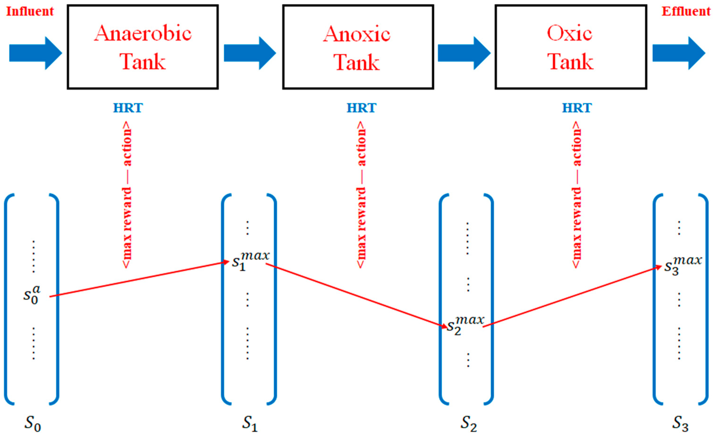
Due to the characteristics of the wastewater treatment processes associated with the successive and coupled reaction units in the AAO system, the effluent concentration vector of the former reaction tank corresponds to the influent concentration vector of the subsequently connected reaction tank. Thus, there are 4 states can be set in the AAO system: $s_0$ is the influent concentration vector of the anaerobic tank; $s_1$ is the influent concentration vector of the anoxic tank (or the effluent concentration vector of the anaerobic tank); $s_2$, is the influent concentration vector of the oxic tank (or the effluent concentration vector of the anoxic tank); $s_3$ is the effluent concentration vector of the oxic tank. For the operation of an AAO system, different control strategies cause different effluent concentrations results. As a direct consequence, in the QL algorithm, different control strategies lead to different transition states, which are represented as s_tⁿ, t ∈ {0, 3}, and four state sets defined as S_t ∈ {s_t¹, s_t^n(t)}. The subscript t of $s_t$ represents the time point corresponds to the influent from the current tank (or the time point corresponds to the effluent from former tank). Therefore, the optimization of the control strategy for the AAO system becomes the state transfer based on the Q matrix.

Figure 2 reports an example of the Q matrix and the corresponding simplified mapping function of AAO system. In Figure 2, each row in the Q matrix is a start state, while each column indicates a transition state. The color of the palette represents the reward under one control strategy, thus different colors correspond to different rewards, which are also distinct control strategies for AAO system. As can be observed in Figure 2, one start state can transfer to many transition states under different control strategies; thus, the Q matrix (or the simplified mapping function) of AAO system is established to choose a strategy to realize the control optimization. Hence, the critical issue is to calculate the transition rewards and then to obtain the pair of <reward-action> (the action in AAO represents the control strategy: HRT and IRR), suggesting that the overall optimization of the control strategy can be realized by following the transition states according to the maximum transition reward (max reward, $s_t^{max}$) in the corresponding state sets (S_t).

Before optimizing the control strategies through the integrated ASM2d-QL algorithm, the continuous concentration data are discretized. Based on the varying concentrations of the influent and the reaction processes in the eight AAO systems, the upper limits of COD (x³), ${\mathrm{NH}}_4^{+}–\mathrm{N}$ (x⁴) and ${\mathrm{PO}}_4^{3-}–\mathrm{P}$. (x⁵) concentrations in this study were set as 500, 50, and 50 mg/L, respectively. The concentrations division intervals of COD, ${\mathrm{NH}}_4^{+}–\mathrm{N}$ and ${\mathrm{PO}}_4^{3-}–\mathrm{P}$ were, respectively, 50, 5, and 0.5 based on the First A level of National Discharge Standard (effluent COD ≤ 50 mg/L, effluent ${\mathrm{NH}}_4^{+}–\mathrm{N}$ ≤ 5 mg/L, and effluent ${\mathrm{PO}}_4^{3-}–\mathrm{P}$ ≤ 0.5 mg/L). According to the Q matrix in Figure 2, the minimum concentration corresponds to state $s_t^1$, while for any other concentration, there is only one corresponding state $s_t^p$, $p\in \left\{1,n\left(t\right)\right\}$. The division of the component concentrations is conducted based on the discretization formula, as shown in Equation (4):

$$p=\left(\lceil \frac{x^3}{50}\rceil -1\right)\times 1000+\left(\lceil \frac{x^4}{5}\rceil -1\right)\times 100+\lceil \frac{x^5}{0.5}\rceil$$

(4)

where $1000=\lceil \frac{50}{5}\rceil \times \lceil \frac{50}{0.5}\rceil$, and $100=\lceil \frac{50}{0.5}\rceil$. The operator “$\lceil \rceil$” represents the rounding up.

In this study, the self-learning of the proposed algorithm is mainly embodied in two aspects. Firstly, owing to the concentration of the component is a continuous parameter and its effluent concentration from each tank varies with different control strategies, the Q matrix composed of <state-value> will automatically update from a sparse matrix to a dense matrix as the number of the simulations increases. The increases in simulation times are achieved by the algorithm itself, and then realize the iteration update of the Q matrix. On the other hand, because of the division of the component concentrations based on the discretization formula (Equation (4)), each state has more corresponding concentrations, while the calculation of the corresponding Q-value is based on the specific concentration. Consequently, there will be multiple values for the same state s. Equipped with the characteristics of self-learning, the proposed algorithm will update the values according to the increases in the number of the simulation times with the maximum reward. When a fluctuating influent load is obtained, the corresponding state of the effluent quality of each tank can be found by searching the maximum reward according to the Q matrix, and then the final overall optimized control strategy can be obtained.

3.2. HRT Optimization Based on ASM2d-Guided Reward

3.2.1. QL Modeling for HRT Optimization

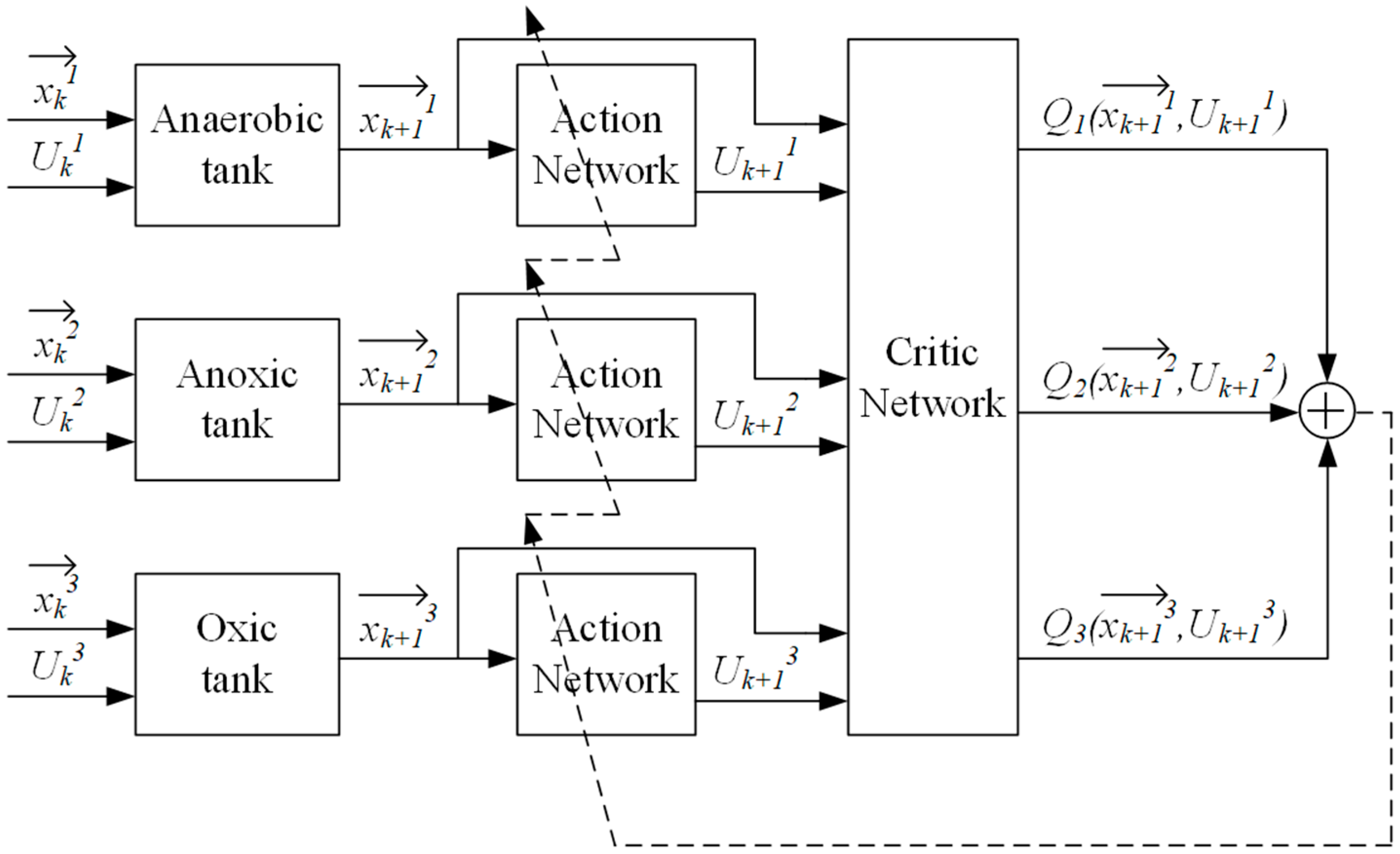
For the AAO system in this study, the concentrations from the three reaction tanks are set as $\overrightarrow{x_k^1}$, $\overrightarrow{x_k^2}$, and $\overrightarrow{x_k^3}$ at a certain time k; $\overrightarrow{x_k^i}=\left(x_k^1,x_k^2\cdot \cdot \cdot x_k^m\right)$ in which i = 1, 2, and 3 denote the three reaction tanks (anaerobic tank, anoxic tank, and oxic tank, respectively) for the AAO system. At time k, the control functions for the three reaction tanks are $U_k^1$, $U_k^2$, and $U_k^3$. Under the same control mode, the corresponding concentrations of $\overrightarrow{x_{k+1}^1}$, $\overrightarrow{x_{k+1}^2}$, and $\overrightarrow{x_{k+1}^3}$ from the three reaction tanks are obtained at time k + 1. Thus, the control functions of $U_{k+1}^1$, $U_{k+1}^2$, and $U_{k+1}^3$ at time k + 1 are obtained according to Action Network. The evaluation function and the Q function for each reaction tank are generated via the QL algorithm. The critic network is further acquired. The logical relationship diagram of the HRT optimal control for the AAO system is depicted in Figure 3. Based on the above analyses, three Q₁, Q₂, and Q₃ functions for each reaction tank, as well as the Q function for the overall AAO system, which are the key to realize the optimal control of the HRTs of the AAO system, could be obtained. This proposed integrated ASM2d-QL algorithm equipped with a self-learning mechanism was gradually formed based on the results of the learning process through a QL algorithm based on the ASM2d model. In the following model development section, the HRTs in anaerobic, anoxic, and oxic tanks of the AAO system with a QL algorithm based on ASM2d were developed and optimized.

3.2.2. ASM2d-Guided Reward Setting in QL Algorithm

For the operation of an AAO system, the optimal control strategy is obtained to reduce all concentration components to the lowest values. Hence, in this case, the Euclidean distance formula, which is widely selected for multi-objective optimization [47], is applied to calculate the evaluation function of the overall descent rate between the descent rate of each component and the minimum descent rate (0%). The evaluation function $V^{\pi }\left(s\right)$ can be calculated with Equation (5):

$$V^{\pi }\left(s\right)=\sqrt{{{\displaystyle \sum _{j=1}^m\left(\frac{{x_{k_0}^j|}_3-{x_0^j|}_1}{{x_0^j|}_1}\right)}}^2}$$

(5)

${x_k^j|}_i$ represents the instantaneous concentration of the jth component in the ith reaction tank at each time k. ${x_{k_0}^j|}_i$ and ${x_0^j|}_i$ represent the effluent and influent concentrations, respectively. The HRT is the reaction time from 0 to k₀. $\pi$ represents the mapping of the control strategy under the corresponding Q-value, and ${\pi }^{*}$ denotes the optimal control strategy based on Equation (2). According to Equation (5), the larger the overall descent rate is (the closer it is to 100%), the better the control strategy can be obtained.

Based on the ASM2d model, Equation (6) can be obtained as follows:

$$\frac{d{x_k^j|}_i}{dk}={\displaystyle \sum _{l=1}^W\left({\rho }_l\cdot {\nu }_l\right)}$$

(6)

where ${\nu }_l$ is the stoichiometric coefficients of the ASM2d, ${\rho }_l$ is the process kinetic rate expression for the component $l$, whereas ${\rho }_l·{\nu }_l$ is composed of $x^1$, $x^2$, …, $x^m$. W is the corresponding reaction processes in ASM2d.

Through integration, Equation (6) can be transformed into Equation (7):

$${\displaystyle {\int }_0^{k_0}\frac{d\left({x_k^j|}_i\right)}{dk}\cdot dk={\displaystyle {\int }_0^{k_0}{\displaystyle \sum _{l=1}^W{\rho }_l\cdot {\nu }_l}\cdot dt}}$$

(7)

Thus, for each reaction tank i, Equation (8) can be obtained as follows:

$${x_{k_0}^j|}_i-{x_0^j|}_i=F_j(\cdot )$$

(8)

where function F_j (·) is the integration of partial differential function for j component in ASM2d, in which the interval of upper and lower bounds of integrals is the HRT.

Based on Equations (5) and (8), the ASM2d-guided reward in QL algorithm can be obtained, as shown in Equation (9):

$$r_i={\displaystyle \sum _{j=1}^m\frac{F_j(\cdot )}{{x_0^j|}_i}}$$

(9)

As HRT becomes the parameter in Equation (9), the reward and HRT can be described as a pair of <reward-HRT>, which indicates that one reward corresponds to one HRT.

The above integrated ASM2d-QL algorithm is described in the pseudo-code of the QL algorithm for the HRTs in the AAO system in

Table 3. Pseudo-code of the QL algorithm for the HRTs in the AAO system.

For each s, t initialize the table entry $\widehat{Q}\left(s,t\right)$ to zero. Observe the current state s While $\left|V^{\pi }\left(s\right)\right|>standard B$ For circulation equals 3 to simulate the whole AAO treatment, do the following: Select an action a and execute it Receive immediate reward r Observe the new state s′ Update the table entry for $\widehat{Q}\left(s,t\right)$ as follows: $$\widehat{Q}\left(s,t\right)=r+\underset{t^{\prime }}{\max }\widehat{Q}\left(s^{\prime },t^{\prime }\right)$$ s ← s′

. The details formula derivation processes are summarized in the supplementary material (see Supplementary Material Section).

3.3. IRR Optimization Based on ASM2d-Guided Reward

IRR optimization is conducted to further obtain the overall optimal control of the whole AAO system. The logical relationship of the control strategy for the IRR optimization is similar to those of the HRTs (Figure 4).

In combination of the above expression and the HRTs optimization process, in one reaction cycle in AAO, the parameter IRR influences the HRTs in anoxic and oxic tanks, whereas the parameter IRR further influences the influent concentrations (${x_0^j|}_i$, i = 2, 3) of the anoxic and oxic tanks. Thus, by combining the pseudo-code of the HRT, the maximum value of the Q function (the optimal control strategy of IRR) can be achieved only through two-time regression.

Hence, based on the above analysis, the integration formula for IRR optimization is shown as Equation (10):

$${\displaystyle {\int }_0^{k_0}\frac{d\left({x_k^j|}_i\right)}{dk}\cdot dk={\displaystyle {\int }_0^{\raisebox{1ex}{$k_0$}\!\left/ \!\raisebox{-1ex}{$q$}\right.}{\displaystyle \sum _{l=1}^W{\rho }_l\cdot {\nu }_l}\cdot dt}}$$

(10)

where q represents the IRR of the AAO system.

Finally, the expression of the ASM2d-guided reward in QL algorithm for IRR optimization based on Equation (10) is obtained, as shown in Equation (11):

$$r_i={\displaystyle \sum _{j=1}^m\frac{G_j(\cdot )}{{x_0^j|}_i}}$$

(11)

where function G_j (·) is the integration of partial differential function in ASM2d for the jth component. Following the same approach used in the HRT optimization in Equation (9), IRR becomes the parameter in Equation (11): thus, the reward and IRR can be described as a pair of <reward-IRR>.

4. Results

4.1. Model Description

To optimize the control strategies of AAO system under varying influent loads based on the proposed ASM2d-QL algorithm, three Q matrixes of the respective anaerobic, anoxic, and oxic tanks have been built for the optimization of HRTs and one Q matrix (one IRR) of the anoxic and oxic reaction tanks has been created for the IRR optimization. Figure 4 depicts the simplified mapping functions for HRTs optimization by the integrated ASM2d-QL algorithm. Because data streams of the influent and effluent concentrations are continuous and that the reward is guided by ASM2d, three simplified mapping functions for respective anaerobic, aerobic, and oxic tanks, instead of the Q matrixes, have been established to choose the optimized control strategies (HRTs) in AAO. In Figure 2, the optimized control strategies of the three HRTs can be calculated through the transition rewards; then, the optimized HRT can be obtained through the pair of <max reward-action>, where action indicates HRT and IRR. By taking the HRT optimization in the anaerobic tank as an example (Figure 4), the influent concentration is $s_0^a$: thus, thanks to the ASM2d-guided reward, the max reward for anaerobic reaction tank can be calculated, while the corresponding HRT can be determined with the pair of <max reward-action>; as a consequence, the effluent concentration will be known as $s_1^{max}$, which is also known as the influent concentration for anoxic reaction tank. Similarly to the HRT optimization of anaerobic tank, the optimized HRTs of anoxic and oxic tanks can be calculated with their own max reward and <max reward-action> pair. By following the transition state transfers from the start state $s_0^a$ to $s_t^{max}$ in the state set S_t, the overall HRT optimization is the combination of the HRTs in each reaction tank.

Similarly, one simplified mapping function can be built to optimize the IRR from start state to transition state for the anoxic and oxic tanks in AAO (Figure 5). Based on the reward calculated by Equation (11), the optimization controlling of IRR can be realized by following the transition state transfers from the start state $s_0^a$ under the control strategy optimized with $s_1^{max}$ in the state set S₁ (Figure 5). Therefore, through the proposed integrated ASM-QL algorithm, the real-time modeling and stable optimal control strategies under fluctuating influent loads (e.g., variations in COD, phosphorus, and nitrogen concentrations) can be obtained by applying the established simplified mapping functions for HRTs and IRR optimization in the AAO system (Figure 4 and Figure 5).

4.2. Model Validation

Experiments and simulation analyses based on eight continuous-flow AAO systems operated under different influent loads (Table 1) were conducted to validate the proposed integrated ASM-QL algorithm. By conducting the iterated and updated optimization of the HRTs through the ASM-QL algorithm, the step length of the control parameters of the HRTs under different reaction tanks in AAO system was set at 0.5 h; the control parameter of the IRR was set as the fixed value of 200% in validation experiments. According to the model developed in Section 3.1, different defined evaluation functions $V^{\pi }\left(s\right)$ correspond to different optimal policies. Herein, we set the evaluation function as $V_{total}^{\pi }\left(s\right)={\displaystyle \sum _{j=3}^5\frac{\left(x_{influent}^j-x_{effluent}^j\right)}{x_{influent}^j}}$ representing the overall maximal removal efficiencies to evaluate the effluent qualities (Equation (4)), where j = 3, 4, and 5 represent S_A, S_NH4, and S_PO4 (Table S2). Then, we utilized the ASM2d-QL algorithms to iterate and update the control parameters of the HRT for all the eight tested systems.

We take here the #1 AAO system as an example to explain how the Q-learning algorithm works with the AAO system optimization under ASM2d-guided reward. Based on the analysis above, we can obtain the pair of <reward-action> for each reaction tank for HRT optimization, which is displayed in Figure 6, with the step of HRT being 0.5 h. The optimized HRT for the AAO system is the combination of the HRT for each reaction tank under its max reward. Therefore, for the #1 influent concentration (Table 1), the combination of HRT is 1 h:2 h:2.5 h (Figure 6), which means that, under that HRT combination, the overall removal efficiency is maximum. The explanation of IRR optimization is similar to the HRT optimization with the step of IRR being 10% times of influent flow rate. From Figure 7 we can observe that the optimized IRR is 260% with the maximum reward.

Table 4. Control strategies of the IRR optimization for #1, #2, …, #8 AAO systems.

Parameters	#1	#2	#3	#4	#5	#6	#7	#8
HRT in anaerobic tank (h)	1.0	0.5	1.5	1.0	2.0	1.0	0.5	1.5
HRT in anoxic tank (h)	2.0	3.5	2.0	3.5	2.5	3.0	2.0	2.5
HRT in oxic tank (h)	2.5	2.0	3.0	3.5	3.5	3.0	3.5	3.5
q (%)	260	310	240	320	290	280	230	250

shows the obtained optimal action-selection policies based on HRTs optimization for the 8 AAO systems. According to the comparison results in Figure 8a₁–c₁, the model simulations and experiment results exhibit similar change tendencies and better fitting degrees. The IRR optimization of the AAO system was further conducted on account of the optimal control strategies of the HRT obtained. Based on Equation (9) and Figure 4, the HRTs for the eight AAO systems were regarded as the fixed values, while the control strategies of the IRR for the eight AAO systems were optimized (Table 4). The model simulations and experimental results for the IRR optimization of the 8 group experiments were finally compared (Figure 8a₂–c₂). As shown in Figure 8a₂–c₂, there is a good agreement between the values of the proposed ASM2d-QL model simulations and the experimental results. To further confirm the goodness-of-fit of the simulation and experiment results after further IRR optimization, we can observe in Figure 8a₂–c₂ that the proposed ASM2d-QL model performed properly and the derived Q functions based on ASM2d successfully realize real-time modeling and stable optimal control strategies under fluctuating influent loads during wastewater treatment.

5. Discussion

5.1. Advantages of the Integrated ASM2d-QL Algorithm

The integrated ASM2d-QL algorithm offers significant advantage of learning mechanisms that can ensure the inherent adaptability for a dynamic environment. In other words, a QL algorithm integrated with mechanistic models can learn from the direct interaction with characteristics of the WWTPs and thus operate considering the practical operation and changeable conditions. Notice that we invest only once in the existing or newly-built WWTPs. Afterwards, the operation of the system with the QL algorithm will adapt to each plant by itself [20]. In this paper, a QL algorithm with ASM2d-guided reward setting is proposed to optimize the control strategies of AAO system under varying influent loads. The verification tests on model performance guarantee the goodness-of-fit of the model and the results (Figure 8). This integrated algorithm provides proper and successful intelligent modeling and stable optimal control strategies under fluctuating influent loads.

5.2. Limitations of the Integrated ASM2d-QL Algorithm

The optimization process of the derived QL algorithm in this study is conducted based on the ASM2d model. However, some restrictive conditions of the ASM2d models, e.g., 20 °C operating temperature, render it not suitable for practical application and changeable conditions. Moreover, other actual influencing factors that affect the selection and operation of WWTPs, such as different influent components, distinct technic characteristics, natural conditions, social situations, even the orientations of process designers, must be taken into account. Therefore, for practical application, whatever it is the lab-, pilot-, or full-scale WWTPs, the data from the ASM2d model by applying this Q function in this study can be replaced with the practically measured values: thus, the actual influencing factors could be taken into consideration. Nowadays, data availability is not the limiting factor for the use of this algorithm due to the development of those real-time data monitoring approaches [17,18,19,25,29]. Through this iterative approach, the Q function based on the practically measured values can be obtained leading to the real-time and precise parameters control.

5.3. Future Developments

This proposed algorithm seems even worthier when we focus on the energy consumption and costs in operation process of the WWTPs. In terms of previous studies [4,31], the optimization of the control process can significantly improve the energy efficiency with very low investments and short payback times. Therefore, a more detailed study on the effect of energy costs is recommended to support decision-makers in future studies. Moreover, more crucial control strategies should be established in this ASM-QL algorithm based on practical applications and specific requirements. In case of environmental changes, a “smart” QL-WWTP can intelligently provide the real-time intelligent decision-making strategies, dynamic optimization control, stable and fast security analysis, and self-healing/self-correction responses without human intervention. It can be envisioned that the QL-WWTPs will become an “ambient intelligence” in all aspects during wastewater treatment.

6. Conclusions

In this study, an integrated ASM2d-QL algorithm was proposed to realize the optimal control strategies of HRTs and IRR in AAO system. To optimize the control strategies under varying influent loads, the simplified mapping functions for HRTs and IRR optimization of AAO system were built based on the proposed ASM2d-QL algorithm. The expressions of the ASM2d-guided reward in QL algorithms for HRTs and IRR optimization were derived. Based on the integrated ASM2d-QL algorithm, the optimized HRTs and IRR were calculated with their own max reward and <max reward-action> pair, respectively. Good agreement between values of the proposed ASM2d-QL model simulations and the experimental results of the eight validation experiments had been proved. This study successfully realizes the intelligent optimization of control strategies under dynamic influent loads through an integrated ASM2d-QL algorithm during wastewater treatment.

References

1. Abbassi, B.E.; Abuharb, R.; Ammary, B.; Almanaseer, N.; Kinsley, C. Modified Septic Tank: Innovative Onsite Wastewater Treatment System. Water 2018, 10, 578. [Google Scholar] [CrossRef]
2. Angelakis, A.N.; Snyder, S.A. Wastewater Treatment and Reuse: Past, Present, and Future. Water 2015, 7, 4887–4895. [Google Scholar] [CrossRef]
3. Jover-Smet, M.; Martín-Pascual, J.; Trapote, A. Model of Suspended Solids Removal in the Primary Sedimentation Tanks for the Treatment of Urban Wastewater. Water 2017, 9, 448. [Google Scholar] [CrossRef]
4. Longo, S.; Mirko d’Antoni, B.; Bongards, M.; Chaparro, A.; Cronrath, A.; Fatone, F.; Lema, J.M.; Mauricio-Iglesias, M.; Soares, A.; Hospido, A. Monitoring and diagnosis of energy consumption in wastewater treatment plants. A state of the art and proposals for improvement. Appl. Energy. 2016, 179, 1251–1268. [Google Scholar] [CrossRef]
5. Zhang, Q.H.; Yang, W.N.; Ngo, H.H.; Guo, W.S.; Jin, P.K.; Dzakpasu, M.; Yang, S.J.; Wang, Q.; Wang, X.C.; Ao, D. Current status of urban wastewater treatment plants in China. Environ. Int. 2016, 92–93, 11–22. [Google Scholar] [CrossRef]
6. Jin, L.Y.; Zhang, G.M.; Tian, H.F. Current state of sewage treatment in China. Water Res. 2014, 66, 85–98. [Google Scholar] [CrossRef]
7. Lu, B.; Huang, S.; Grossmann, I.E. Optimal Synthesis and Operation of Wastewater Treatment Process with Dynamic Influent. Ind. Eng. Chem. Res. 2017, 56, 8663–8676. [Google Scholar] [CrossRef]
8. Jiang, Y.; Dinar, A.; Hellegers, P. Economics of social trade-off: Balancing wastewater treatment cost and ecosystem damage. J. Environ. Manag. 2018, 211, 42–52. [Google Scholar] [CrossRef]
9. Zuluaga-Bedoya, C.; Ruiz-Botero, M.; Ospina-Alarcón, M.; Garcia-Tirado, J. A dynamical model of an aeration plant for wastewater treatment using a phenomenological based semi-physical modeling methodology. Comput. Chem. Eng. 2018, 117, 420–432. [Google Scholar] [CrossRef]
10. Nourani, V.; Elkiran, G.; Abba, S.I. Wastewater treatment plant performance analysis using artificial intelligence-an ensemble approach. Water Sci. Technol. 2018, 78, 2064–2076. [Google Scholar] [CrossRef] [PubMed]
11. Han, H.G.; Qian, H.H.; Qiao, J.F. Nonlinear multiobjective model-predictive control scheme for wastewater treatment process. J. Process Contr. 2014, 24, 47–59. [Google Scholar] [CrossRef]
12. Henze, M.; Gujer, W.; Mino, T.; van Loosedrecht, M. Activated Sludge Models ASM1, ASM2, ASM2d and ASM3; IWA Scientific and Technical Report No. 9; IWA Publishing: London, UK, 2000. [Google Scholar]
13. Drewnowski, J.; Makinia, J.; Szaja, A.; Łagód, G.; Kopeć, Ł.; Aguilar, J.A. Comparative Study of Balancing SRT by Using Modified ASM2d in Control and Operation Strategy at Full-Scale WWTP. Water 2019, 11, 485. [Google Scholar] [CrossRef]
14. Wu, X.H.; Yang, Y.; Wu, G.M.; Mao, J.; Zhou, T. Simulation and optimization of a coking wastewater biological treatment process by activated sludge models (ASM). J. Environ. Manag. 2016, 165, 235–242. [Google Scholar] [CrossRef] [PubMed]
15. Yang, S.S.; Pang, J.W.; Guo, W.Q.; Yang, X.Y.; Wu, Z.Y.; Ren, N.Q.; Zhao, Z.Q. Biological phosphorus removal in an extended ASM2 model: Roles of extracellular polymeric substances and kinetic modeling. Bioresour. Technol. 2017, 232, 412–416. [Google Scholar] [CrossRef] [PubMed]
16. Harrou, F.; Dairi, A.; Sun, Y.; Senouci, M. Statistical monitoring of a wastewater treatment plant: A case study. J. Environ. Manag. 2018, 223, 807–814. [Google Scholar] [CrossRef] [PubMed]
17. Chow, C.; Saint, C.; Zappia, L.; Henderson, R.; Roeszler, G.; Dexter, R.; Nguyen, T.; Stuetz, R.; Byrne, A.; Trolio, R.; et al. Online water quality monitoring-the voice of experience, meeting the challenges and removing barriers to implementing online monitoring schemes. AWA Water J. 2014, 41, 60–67. [Google Scholar]
18. Chow, C.W.K.; Liu, J.; Li, J.; Swain, N.; Reid, K.; Saint, C.P. Development of smart data analytics tools to support wastewater treatment plant operation. Chemometr. Intell. Lab. 2018, 177, 140–150. [Google Scholar] [CrossRef]
19. Van den Broeke, J.; Carpentier, C.; Moore, C.; Carswell, L.; Jonsson, J.; Sivil, D.; Rosen, J.S.; Cade, L.; Mofidi, A.; Swartz, C.; et al. Compendium of Sensors and Monitors and Their Use in the Global Water Industry; Water Environment Research Foundation: Alexandria, VA, USA; Global Water Research Coalition: Unley, SA, Australia, 2014. [Google Scholar]
20. Hernández-del-Olmo, F.; Llanes, F.H.; Gaudioso, E. An emergent approach for the control of wastewater treatment plants by means of reinforcement learning techniques. Expert Syst. Appl. 2012, 39, 2355–2360. [Google Scholar] [CrossRef]
21. Hreiz, R.; Latifi, M.A.; Roche, N. Optimal design and operation of activated sludge processes: State-of-the-art. Chem. Eng. J. 2015, 281, 900–920. [Google Scholar] [CrossRef]
22. Al Jibouri, A.K.H.; Upreti, S.R.; Wu, J. Optimal control of continuous ozonation of non-biodegradable pollutants. J. Process Contr. 2018, 66, 1–11. [Google Scholar] [CrossRef]
23. De Araújo, A.C.B.; Gallani, S.; Mulas, M.; Olsson, G. Systematic approach to the design of operation and control policies in activated sludge systems. Ind. Eng. Chem. Res. 2011, 50, 8542–8557. [Google Scholar] [CrossRef]
24. Machado, V.C.; Gabriel, D.; Lafuente, J.; Baeza, J.A. Cost and effluent quality controllers design based on the relative gain array for a nutrient removal WWTP. Water Res. 2009, 43, 5129–5141. [Google Scholar] [CrossRef] [PubMed]
25. Gopakumar, V.; Tiwari, S.; Rahman, I. A deep learning based data driven soft sensor for bioprocesses. Biochem. Eng. J. 2018, 136, 28–39. [Google Scholar] [CrossRef]
26. Han, H.G.; Liu, Z.; Guo, Y.N.; Qiao, J.F. An intelligent detection method for bulking sludge of wastewater treatment process. J. Process Contr. 2018, 68, 118–128. [Google Scholar] [CrossRef]
27. Shi, S.; Xu, G. Novel performance prediction model of a biofilm system treating domestic wastewater based on stacked denoising auto-encoders deep learning network. Chem. Eng. J. 2018, 347, 280–290. [Google Scholar] [CrossRef]
28. Torregrossa, D.; Leopold, U.; Hernández-Sancho, F.; Hansen, J. Machine learning for energy cost modelling in wastewater treatment plants. J. Environ. Manag. 2018, 223, 1061–1067. [Google Scholar] [CrossRef]
29. Zhu, J.; Kang, L.; Anderson, P.R. Predicting influent biochemical oxygen demand: Balancing energy demand and risk management. Water Res. 2018, 128, 304–313. [Google Scholar] [CrossRef]
30. Guo, H.; Jeong, K.; Lim, J.; Jo, J.; Kim, Y.M.; Park, J.P.; Kim, J.H. Prediction of effluent concentration in a wastewater treatment plant using machine learning models. J. Environ. Sci. China 2015, 32, 90–101. [Google Scholar] [CrossRef]
31. Guerrini, A.; Romano, G.; Indipendenza, A. Energy Efficiency Drivers in Wastewater Treatment Plants: A Double Bootstrap DEA Analysis. Sustainability 2017, 9, 1126. [Google Scholar] [CrossRef]
32. Turunen, V.; Sorvari, J.; Mikola, A. A decision support tool for selecting the optimal sewage sludge treatment. Chemosphere 2018, 193, 521–529. [Google Scholar] [CrossRef]
33. Marvuglia, A.; Kanevski, M.; Benetto, E. Machine learning for toxicity characterization of organic chemical emissions using USEtox database: Learning the structure of the input space. Environ. Int. 2015, 83, 72–85. [Google Scholar] [CrossRef] [PubMed]
34. Mesbah, M.; Soroush, E.; Rezakazemi, M. Development of a least squares support vector machine model for prediction of natural gas hydrate formation temperature. Chin. J. Chem. Eng. 2017, 25, 1238–1248. [Google Scholar] [CrossRef]
35. Vamvoudakis, K.G.; Mojoodi, A.; Ferraz, H. Event-triggered optimal tracking control of nonlinear systems. Int. J. Robust Nonlin. 2017, 27, 598–619. [Google Scholar] [CrossRef]
36. Wei, Q.L.; Liu, D.R.; Shi, G. A Novel Dual Iterative Q-Learning Method for Optimal Battery Management in Smart Residential Environments. IEEE Trans. Ind. Electron. 2015, 62, 2509–2518. [Google Scholar] [CrossRef]
37. Wei, Q.L.; Song, R.Z.; Sun, Q.Y. Nonlinear neuro-optimal tracking control via stable iterative Q-learning algorithm. Neurocomputing 2015, 168, 520–528. [Google Scholar] [CrossRef]
38. Kiumarsi, B.; Lewis, F.L.; Modares, H.; Karimpour, A.; Naghibi-Sistani, M.B. Reinforcement-learning for optimal tracking control of linear discrete-time systems with unknown dynamics. Automatica 2014, 50, 1167–1175. [Google Scholar] [CrossRef]
39. Wang, K.; Chai, T.Y.; Wong, W.C. Routing, power control and rate adaptation: A Q-learning-based cross-layer design. Comput. Netw. 2016, 102, 20–37. [Google Scholar] [CrossRef]
40. Syafiie, S.; Tadeo, F.; Martinez, E.; Alvarez, T. Model-free control based on reinforcement learning for a wastewater treatment problem. Appl. Soft Comput. 2011, 11, 73–82. [Google Scholar] [CrossRef]
41. Zhang, W.T.; Hou, F.; Peng, Y.Z.; Liu, Q.S.; Wang, S.Y. Optimizing aeration rate in an external nitrification–denitrifying phosphorus removal (ENDPR) system for domestic wastewater treatment. Chem. Eng. J. 2014, 245, 342–347. [Google Scholar] [CrossRef]
42. Fang, F.; Qiao, L.L.; Cao, J.S.; Li, Y.; Xie, W.M.; Sheng, G.P.; Yu, H.Q. Quantitative evaluation of A2O and reversed A2O processes for biological municipal wastewater treatment using a projection pursuit method. Sep. Purific. Tech. 2016, 166, 164–170. [Google Scholar] [CrossRef]
43. APHA (American Public Health Association). Standard Methods for the Examination of Water and Wastewater, 21st ed.; APHA: Washington, DC, USA, 2005. [Google Scholar]
44. Watkins, C. Learning from Delayed Rewards. Ph.D. Thesis, Cambridge University, Cambridge, UK, 1989. [Google Scholar]
45. Watkins, C.; Dayan, P. Q-learning. Mach. Learn. 1992, 8, 279–292. [Google Scholar] [CrossRef]
46. Arin, A.; Rabadi, G. Integrating estimation of distribution algorithms versus Q-learning into Meta-RaPS for solving the 0–1 multidimensional knapsack problem. Comput. Ind. Eng. 2017, 112, 706–720. [Google Scholar] [CrossRef]
47. Mitchell, T.M. Machine Learning; McGraw-Hill Science/Engineering/Math: New York, NY, USA, 1997; pp. 367–379. ISBN 0070428077. [Google Scholar]
Figure 1. The schematic flow diagram of the continuous-flow anaerobic/anoxic/oxic (AAO) systems for model validation.
Water 11 00927 g001
Figure 2. An example of the Q matrix and the corresponding simplified mapping function of the AAO system.
Water 11 00927 g002
Figure 3. The logical relationship diagram of the HRTs optimal control for the AAO system.
Water 11 00927 g003
Figure 4. Simplified mapping functions for HRTs optimization in AAO system by an integrated ASM-QL algorithm.
Water 11 00927 g004
Figure 5. Simplified mapping function for IRR optimization in AAO system by an integrated ASM-QL algorithm.
Water 11 00927 g005
Figure 6. The pair of <reward-action> for HRTs optimization for (a) anaerobic tank, (b) anoxic tank, and (c) oxic tank.
Water 11 00927 g006
Figure 7. The pair of <reward-action> for IRR optimization.
Water 11 00927 g007
Figure 8. Model simulations and experimental results for eight AAO systems: (a1,a2) COD effluent concentrations; (b1,b2) NH4-N effluent concentrations; and (c1,c2) TP effluent concentrations of the HRTs optimization and the IRR optimization.
Water 11 00927 g008aWater 11 00927 g008b