Next Article in Journal
Opportunities and Challenges for the Sustainability of Lakes and Reservoirs in Relation to the Sustainable Development Goals (SDGs)
Previous Article in Journal
Spatial–Temporal Matching Characteristics between Agricultural Water and Land Resources in Ningxia, Northwest China
 
 
Correction published on 3 February 2020, see Water 2020, 12(2), 408.
Article

Combination of Discrete Element Method and Artificial Neural Network for Predicting Porosity of Gravel-Bed River

1
Institute of Hydraulic and Water Resources Engineering, Technische Universität München, Arcisstrasse 21, D-80333 München, Germany
2
Faculty of Mechanical Engineering, Thuyloi University, 175 Tay Son, Dong Da, Hanoi 100000, Vietnam
*
Author to whom correspondence should be addressed.
Water 2019, 11(7), 1461; https://doi.org/10.3390/w11071461
Submission received: 12 June 2019 / Revised: 5 July 2019 / Accepted: 12 July 2019 / Published: 14 July 2019
(This article belongs to the Section Hydraulics and Hydrodynamics)

Abstract

:
In gravel-bed rivers, monitoring porosity is vital for fluvial geomorphology assessment as well as in river ecosystem management. Conventional porosity prediction methods are restricting in terms of the number of considered factors and are also time-consuming. We present a framework, the combination of the Discrete Element Method (DEM) and Artificial Neural Network (ANN), to study the relationship between porosity and the grain size distribution. DEM was applied to simulate the 3D structure of the packing gravel-bed and fine sediment infiltration processes under various forces. The results of the DEM simulations were verified with the experimental data of porosity and fine sediment distribution. Further, an algorithm was developed for calculating high-resolution results of porosity and grain size distribution in vertical and horizontal directions from the DEM results, which were applied to develop a Feed Forward Neural Network (FNN) to predict bed porosity based on grain size distribution. The reliable results of DEM simulation and FNN prediction confirm that our framework is successful in predicting porosity change of gravel-bed.

1. Introduction

The significantly different size of fine sediment and coarse bed material is the reason for the change in the void space of gravel-bed rivers. If finer sediments occupy the interstitial spaces of coarser bed materials, the void space of the bed material decreases. If finer sediments are supplied at a small rate to a riverbed covered by a completely developed armor coat, the fine sediments can infiltrate into the interstitial spaces of the coarser bed material and move into void spaces. As a result of fine sediment exchange in void space, the ratio of void space over the total amount of gravel-bed and the porosity change [1,2]. The study of porosity variation plays an important role for fluvial geomorphology assessment and in river ecosystem management. From a river management point of view, the amount of fine sediment stored in the void space of the gravel-bed up to 22% may be neglected and porosity can be considered constant [1]. The impact the void spaces of gravel-bed have on habitats for fish and aquatic species are substantial, and are of important considerations in assessing changes in the void structure of bed materials [3]. Morphologically, the porosity strongly influences the rate of bed level changes [4,5]. The reduction of porosity due to the excess of fine sediment prevents hydrologic exchange surface and underground water [6]. Hence, the variation of the bed porosity should be considered in hydromorphological models for gravel-bed rivers and also in defining hydrological conductivity of modeling of ground water [7,8].
Porosity predictions for fluvial gravel-bed mixtures are classified into two types: Empirical prediction and theoretical prediction. The empirical prediction focuses mainly on the relationship between porosity and grain size [9,10,11]. Carling and Reader [12] studied the sedimentological properties upland streams in Britain, concentrating on consolidated, clast-supported gravel deposits with that had varying infills of sand and silt. A strong relation between porosity and median grain size was observed. Wu and Wang [9] revaluated previously collected laboratory and field data to improve the earlier porosity prediction made earlier by Komura [13]. In order to produce unimodal sand-gravel mixtures, Wooster et al. [10] mixed together grains ranging from 0.075 to 22 mm in size. After slight compaction of the samples, the porosity of the mixtures were found to be correlated to the standard deviation of the distribution of grain sizes. Peronius and Sweeting [11] had developed a quite different method of empirically predicting porosity. The impact grain shape on porosity was introduced and a Kolmogorov-Smirnov statistic was used to articulate the grain size. Porosity measurements in densified, artificially packed, and cohesionless mixtures were the basis for their predictor. An advantage of empirical predictions is that they are largely based on porosity measurements in natural sediments and are easy to apply because of their simple form; however, they cannot be confidently used in areas different than the original study area. Due to the limiting number of control factors considered (only median grain size and deviation of the grain size distribution), there is an overestimation of the porosity for almost uniform sediments when using the porosity calculation based on the relation between the sediment standard deviation. The porosity calculation based on the grain size distribution’s deviation, which leads to an increase in porosity seems valid, however, it does not result in an accurate porosity prediction [14].
Theoretical packing models exist that can be used to predict porosity in addition to the empirical predictors, as mentioned before. Most of theoretical models are derived from laboratory experiments with spherical grains and simple packing techniques (often consisting of only two size fractions). Early theoretical packing models simulated either the mixing process occupation or the mixing process filling [15]. Filling effects and occupation effects occur simultaneously in natural sediment mixtures containing a large range of grain sizes. Yu and Standish [16,17], who have produced one of the best performances for porosity prediction of sand gravel-bed [14], developed a method for predicting porosity for continuous grain size distributions that considers both mixing processes simultaneously. This mathematical model has required experimental coefficients and was recently verified for the binary mixture. A random-packing computer model of spherical particles, mainly used in the research field of powder technology, is a valuable tool towards obtaining porosity. Suzuki and Oshima [18] employed a random-packing model to find the positions of particles in a vessel by dropping and rolling. Nolan and Kavanagh [19] improved a random-packing model for a lognormal distribution. Kenneth and Weeks [20] developed a different random packing model to obtain the packing fraction. The significant time consumption of these processes leads to a difficultly in their application in a large domain or their integration into other calculation systems that requires the porosity recalculation at every time step of the size fraction change.
In recent decades, Artificial Neural Network (ANN), a computational intelligence technique, has been emerged as a powerful tool for handling the complex geoscience, and morphology problems [21,22]. Porosity prediction using ANN mostly originates from the field of petroleum engineering to investigate carbonate reservoirs based on well-log data (used the acoustic, nuclear, resistivity technology, sonic transit time, and density logs to obtain the porosity indirectly) [23,24,25]. Due to using the indirect measurement method and using many conversation formulas [21], porosity data obtained by well-log data has high errors and low resolution (porosity value is usually approximated in few meters). These prevented the application of ANN in predicting porosity of gravel-bed river where bed thickness is much smaller than carbonate reservoirs. However, with a high resolution of data, the porosity prediction from ANN enables us to overcome two weak points of empirical and theoretical porosity prediction in gravel-bed rivers, including limited multi controlling factor, and computation time.
Presently, Bui et al. [7] have developed a numerical hydromorphological model considering bed porosity changes and exchange fluxes of fine sediment between two different bed layers. The change in the bed elevation is calculated based on the mass conservation in the active layer. The grain sorting in the active layer occurs under the flow interaction and exchange processes occurring between the active layer and the active stratum layer. The grain sorting of the active stratum layer is only caused by the exchange process between these two layers. Further, the exchange rate for the fine fraction of size class can be quantified, based on the empirical equation of Toro-Escobar et al. [26]. After defining the grain size distribution, the bed porosity is calculated using the semi-empirical equations proposed by Reference [16]. This equation required an empirical coefficient and was verified for binary mixture. Therefore, the porosity calculation model needs to reduce computational time as well as increase accuracy by taking into account the change of multi size fraction of bed material.
In this study, a framework combining the Discrete Element Method (DEM) and Artificial Neural Network (ANN) was introduced to predict the porosity of gravel-bed rivers. Firstly, DEM was applied to simulate the 3D bed structure formed by fine sediment infiltrating into gravel packing bed. Then, the results of porosity and sediment distributions obtained by the DEM were compared with experimental results to confirm the capacity of the DEM model. An algorithm was developed for calculating porosity and grain size distribution by the depth of flumes and along the flume. Finally, datasets obtained by the DEM model were used to design an ANN model, called Feed Forward Neural Network (FNN), for predicting the bed porosity of gravel-bed river.

2. Methodology

In this study, we weave multiple techniques together into one platform, which is shown in Figure 1. The detailed implementation of each component is presented in the following subsections.

2.1. Discrete Element Method (DEM)

The Discrete Element Method (DEM) was initially suggested by Cundall and Strack [27] to model the mechanical behavior of granular flows and to simulate the forces acting on each particle and its motion. Typically, a particle can be classified into two types of motion in DEM: Translation and rotation. Momentum and energy of particles are exchanged during collisions with their neighbors or a boundary wall (contact forces), and particle-fluid interactions, as well as gravity. Through the application of Newton’s second law of motion, we can determine the trajectory of each i-particle (including its acceleration, velocity, and position) from the following equations:
m i d u i dt   = m i g + k f i , k + f i , f
I d ω i dt = d i 2 k ( n i , k × f i , k )
where mi = the mass of a particle i; u i = the velocity of a particle; g = Gravity acceleration; f i , k = interaction force between particle i and particle k (contact force); f i , f = interaction force between the particle i and the fluid; I = moment of inertia; ω i = angular velocity; di = diameter of the grain i; and n i , k = directional contact = vector connecting the center of grains i and k.
We use a contact force model based on the principle of spring-dashpot as well as suggestions of Hertz-Mindlin [28]. The contact force is obtained from a force analysis method; the stiffness and damping factors are analyzed in two directions: Orthogonal and tangent of the contact surface between the two grains (Figure 2):
f i , k ( n )   = k i ( n ) δ i , k ( n )   + α i ( n ) Δ u i ( n ) .
f i , k ( τ )   = k i ( τ ) δ i , k ( τ )   + α i ( τ ) Δ u i ( τ )
(n) and (τ) are known as two components of contact force in normal and tangential directions; ki = stiffness of grain i; δi,k = the characteristic of the contact and displacement (also called the length of the springs in the two directions above); αi = damping coefficient; and Δui = relative velocity of grain at the moment of collision. Following Coulomb, the value of tangential friction is determined by the product of the friction coefficient μ and the orthogonal force component. In the nonlinear contact force, Hertz-Mindlin model, the tangential force component will increase until the ratio (f(τ)/f(n)) reaches a value of μ, and it retains the maximum value until the particles are no longer in contact with each other. A detail of the force models, as well as the method for determining the relevant coefficients, can be found in Reference [28].
After calculating all forces acting on the sediment particles as well as the velocity and the position of the particle at a previous time step, we can determine the current velocity and position of grain by solving Equations (3) and (4). The grain size distribution, as well as the bed porosity for whole the domain, can be defined afterward. As a result, we can also estimate the exchange rate of the fine fraction between different bed layers.
The DEM simulations begin with defining the system geometry. This comprises boundary conditions, particle coordinates, and material properties by identifying the contact model parameters, such as the friction and stiffness coefficients. How loading or deforming occurs within the system can be determined by the user through adding loads, deformations, or settlements. The simulation begins as either a transient or dynamic analysis and runs until the completion of a defined number of time steps. An overlap check procedure starts after particles are inserted into the simulation box, which is conducted based on the geometry and coordinates of the particles. Upon the simulation of motions starting, particles that physically encounter each other are detected, and the contact forces are then calculated at each time step. The magnitude of particle forces is related to the distance between the each of the contacting particles. From this data, the resultant force including, body forces, external forces, and moment acting on each particle can be calculated.
Moreover, two sets of equations for the dynamic equilibrium of the particles are computed in the case when particle rotation is blocked. Each particle translational movement is derived from the resultant applied force and each particle rotational movement is formulated from the resultant applied moment. By knowing the inertia of the particles, particle translational, and rotational accelerations can be calculated. After new contract forces are determined, the particle positions and orientations are updated and ready for the next time step and will be repeated for all time steps. While this system seems to respond in an almost static manner, the Discrete Element Method is a transient or dynamic analysis.
Figure 3 shows the calculation series that occur within a given time step. Particle velocities and incremental displacements are the first to be calculated. Here, the equilibrium of each particle in the sequence is considered. In the second series of calculations, upon the system geometry being updated, the forces at each contact in the whole system are then calculated. The particle rotational moment is produced from the normal contact force, as well as the tangential component of the contact force. As the output of these calculated moments and forces, the new particle position is generated for the next time step, and the series of calculation begins again. For every particle-based DEM simulation, the following fundamental assumptions are accepted. The first consideration is that particles are rigid, each possessing a finite inertia that can be described analytically. Moreover, the particles can translate and rotate independently of each other. The detections of new particle contacts are automatically completed by a geometry check algorithm. Physical contacts of particles normally happen over an infinitesimally small area based on the allowed overlapping and consists of only two particles. Particles that interact in DEM simulations are authorized to overlap slightly at the contact point, where the magnitude of the overlap is required to be small. The compressive inter-particle forces can be calculated from the particles overlapping value. Tensile and compression forces can be transferred at particle contact points and is normal in the direction of contact, as well as a tangential force orthogonal to the normal contact force. Furthermore, there is distance between two separating particles where the tensile inter-particle forces are calculated. When particles collide, this force is its maximum value, and then the particles move away from each other, which also means that the contact area diminishing to zero and is no longer used in contact force calculations. The last key assumption is that clusters of the rigid base particles can be used to represent a single particle. A measurable deformation of the composite particles is caused by the relative motion of the base particles within the cluster. These particle agglomerates may also be rigid themselves.
In this study, we used the open Source Discrete Element Method Particle Simulation (LIGGGHTS) implemented a new Hertz-Mindlin granular contact model [28,30,31], where grains are modeled as compressible spheres with a diameter d that interacts when in contact via the Hertz-Mindlin model [28,30,31]. An algorithm was developed to calculate grain size distribution and porosity from the calculated results of location and diameter of grains.
Defining a simulation time step is one of many essential steps in setting up the DEM. Sufficiently short time steps ensure stability of the system and enable stimulation of the real processes. According to Johnson [27,28], disturbances that occur during motion of particles in a granular system propagate following the Rayleigh waves form along the surface of solid. The simulation time step is included in the Rayleigh time, which is the time the energy wave takes to transverse the smallest element in the system. The simulation time step should be small enough so that any disturbance of a particle’s motion only propagates to its nearest neighbors. Velocity and acceleration are assumed to be constant during the time step. Moreover, the time step duration should be smaller than the critical time increment evaluated from theory. Several equations have been proposed for calculating a critical time step [27]. In this study, we applied a time step of 0.00001 s, which is smaller than 20 percent of the Rayleigh time.

2.2. Algorithms for Calculating Grain Size Distribution and Porosity of a Cross Section from DEM Results

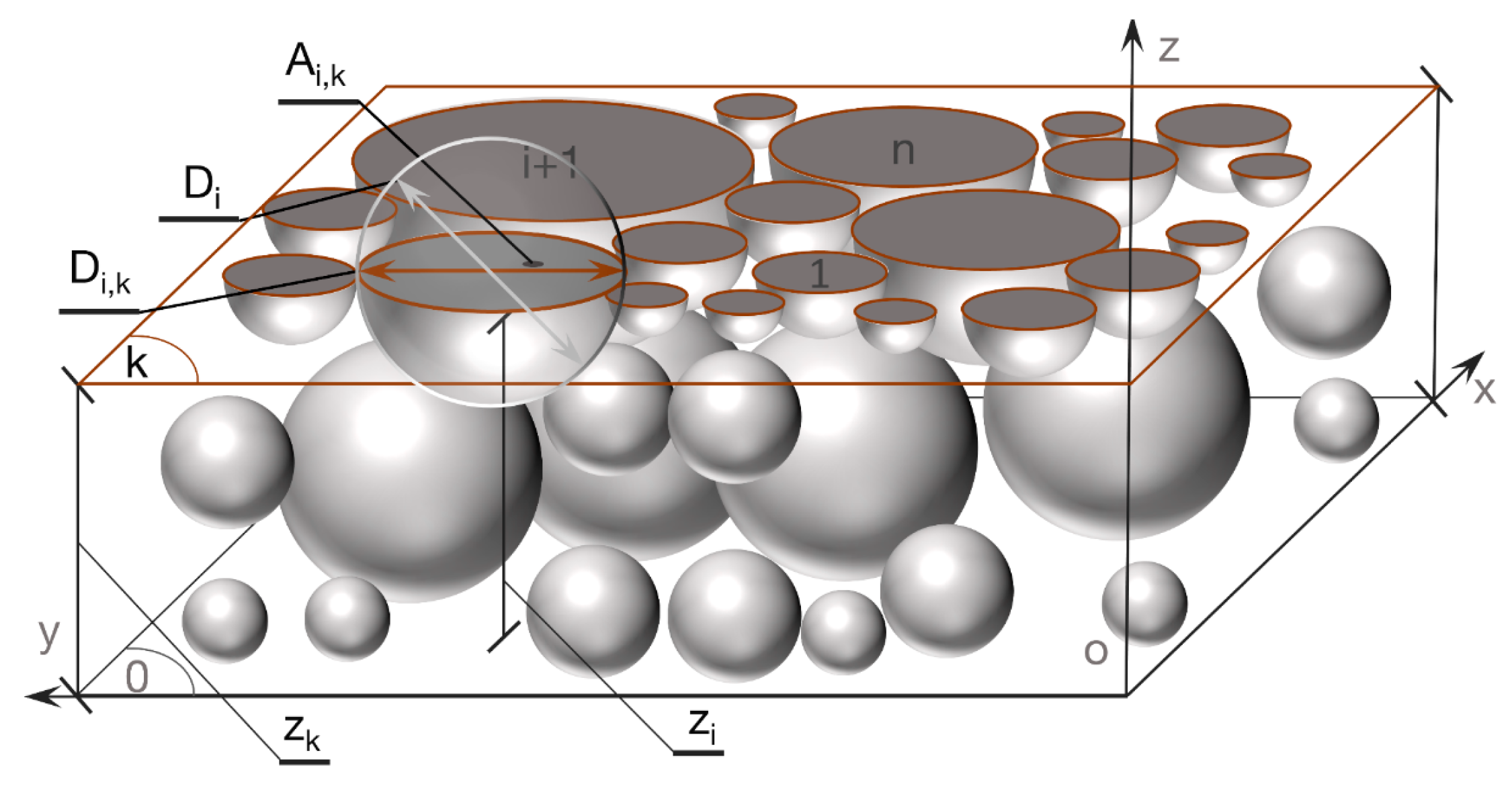
The results obtained from LIGGGHTS, an open source Discrete Element Method particle simulation software, contains 3D locations and diameter of grains. To calculate the porosity and grain size distribution, a simple algorithm was developed. We used the K different planes with elevations zk (k = 0, …, K), which intersect the spherical grain matrix. The diameter of generated circle i (i = 1, …, nk) is dependent on the spherical diameter and the relative position between the k-plane and grain i (Figure 4).
The diameter of each circle created by the intersection between plane k and grain ith is calculated as:
D i , k =   D i 2     4 ( z k z i ) 2   if   z i   D i 2   z k < z i +   D i 2
Total solid area (As,k) of all nk grains in plane k is determined:
A s , k   =   i = 1 n k A i , k =   i = 1 n k π D i , k 2 4
The total area At is calculated based on the shape generated by the plane k cut across the grain matrix, whereby porosity of cross section k is calculated by the following equation:
p k = 1   A s , k A t
To calculate the grain size distribution, the grains in cross-section k are divided into mk size fractions with characteristic grain size Dj (j = 1, …, mk) and Dj < Dj+1, then the area of each fraction is calculated by
A j ( k )   =   i = 1 n j , k π D i , k 2 4   if   D j 1 D i , k < D j
With
j = 1 m k n j , k = n k
The fraction of class j in cross-section k is calculated by the following equation:
β j ( k ) = A j ( k ) i = 1 m k A i ( k )

2.3. Feed Forward Neural Network (FNN)

Artificial Neural Network (ANN) is a general term encompassing many different network architectures. A Feedforward Neural Network (FNN) is an artificial neural network where connections between nodes do not form a cycle [32]. FNN is the first and simplest type of artificial neural network developed. Information of an FNN travels in only one direction, forward, from input nodes, through hidden nodes, then to the output nodes. Further, the most widely used FNN is a multilayer perceptron (MLP). An MLP model contains several artificial neurons otherwise known as processing elements or nodes. A neuron is a mathematical expression that filters signals traveling through the net. An individual neuron receives its weighted inputs from the connected neurons of the previous layer, which are normally aggregated along with a bias unit. The bias unit is purposed to scale the input to a useful range to improve the convergence properties of the neural network. The combined summation is delivered through a transfer function to generate the neuron output. Weighted connections modify the output as it is passed to neurons in the next layer, where the process is repeated. The weight vectors that connect the different network nodes are discovered through the so-called error back-propagation method. During training, these parameters values are varied in order for the FNN output to align with the measured output of a known dataset [33,34]. Changing the connections’ weights in the network, according to an error minimization criterion, achieves a trained response. Overfitting is avoided if a validation process is implemented during the training. When the network has been sufficiently trained to simulate the best response to input data, the network configuration is fixed and a test process is conducted to evaluate the performance of the FNN as a predictive tool [22].
In feed-forward networks (Figure 5), messages are passed forward only. A network with L layers has a parameter and a differentiable function f ( l )   :   R d 1   R d 1 corresponding to the lth layer. Given an input x ∈ R d o , the network outputs:
W ( l )   R d l × d l 1   y     a ( L )
where each a ( l )   R d l is defined and is defined recursively from the base case a ( 0 ) x as follows:
z ( l )   W ( l ) a ( l 1 ) a ( l ) f ( l ) z ( l )
The training process minimizes a loss function l :     R d L × d L     R over labeled examples (x, y). The gradient of the squared loss on (x, y) with respect to W(L) is
W ( L ) [ 1 2 | | y     a ( L ) | | 2 ] = [ ( a ( L )   y ) f ( L ) ( z ( L ) ) ] ( a ( L 1 ) ) T
The form mirrors the delta rule because a ( L ) = f ( L ) ( W ( L ) a ( L 1 ) ) T where a ( L 1 ) does not involve W ( L ) . By defining the “error term”,
δ ( L ) ( a ( L ) y ) f ( L ) ( z ( L ) )
we can simplify Equation (14) as δ ( L ) ( a ( L 1 ) ) T . Similarly, the gradient with respect to W ( l ) for l < L can be verified to be δ ( l ) ( a ( l 1 ) ) T where
δ ( l ) f ( l ) ( z ( l ) ) ( W ( l + 1 ) T δ ( l + 1 ) )
Computing all gradients in a multi-layer network in this manner is commonly known as “backpropagation”, which is just a special case of automatic differentiation. For concreteness, here is the backpropagation algorithm for an L-layer feedforward network with the squared loss
Input labeled example ( x , y ) = R d L × R d L parameters { W ( l ) } l = 1 L
Output:
W ¯ ( l ) W ( l ) [ 1 2 | | y a ( L ) | | 2 ]   for   l = 1 , ,   L
Feedforward phase
Set a ( 0 ) x , and for l = 1, …, L compute:
z ( l )   W ( l ) a ( l 1 ) a ( l )   f ( l ) z ( l )
Backpropagation phase
Set δ ( L ) ( a ( L ) y ) f ( L ) ( z ( L ) ) , and for l = L−1, …, 1 compute:
δ ( l ) f ( l ) ( z ( l ) ) ( W ( l + 1 ) T δ ( l + 1 ) )
Set W ¯ ( l ) δ ( l ) ( a ( l 1 ) ) T , and for l = 1, …, L.
The optimization algorithm (or optimizer) is the main approach used for training a machine-learning model to minimize its error rate. There are two metrics to determine the efficacy of an optimizer: Speed of convergence (the process of reaching a global optimum for gradient descent); and generalization (the model’s performance on new data). Popular algorithms such as Adaptive Moment Estimation (Adam) or Stochastic Gradient Descent (SGD) can capably cover one or the other metric. The Adam optimizer, presented by Kingma and Ba [35], is extensively used for deep learning models requiring first-order gradient-based descent with small memory and the ability to compute adaptive learning rates for different parameters [36]. This method is computationally efficient, easy to implement, and has proven to perform better than the RMSprop and Rprop optimizers [37]. Gradient rescaling is reliant on the magnitudes of parameter updates. The Adam optimizer does not require a stationary object and can work with more sparse gradients. We calculate the decaying averages of past and past squared gradients m t and v t , respectively, as follows:
m t = β 1 m t 1 + ( 1 β 1 ) g t
v t = β 2 v t 1 + ( 1 β 2 ) g t 2
m t and v t are estimates of the first moment (the mean) and the second moment (the uncentered variance) of the gradients, respectively. m t and v t are initialized as vectors of 0, the authors of Adam noticed that they are biased towards zero, particularly during the initial time steps and during smaller decay rates (i.e., β 1 and β 2 are close to 1).
Bias-corrected first and second moment estimates are computed to counteract these biases:
m ^ t = m t 1 β 1 t
v ^ t = v t 1 β 2 t
Parameters are then updated by:
θ t + 1 = θ t   η v ^ t + ϵ 1 m ^ t
The default value in this study: β 1 = 0.9 , β 2 = 0.999 and ϵ = 10 8 with learning rate = 0.001. More detail about this method is available in Reference [35]
To create the FNN architecture, one must first determine the number of layers of each type and the number of nodes in each of these layers. In an FNN, one or more hidden layer of sigmoid neurons are often found, subsequently followed by an output layer containing linear neurons or nodes. This is completed because by having multiple layers of neurons with nonlinear activation functions, it allows the network to learn nonlinear relationships that exist between input and output vectors [38]. There is debate surrounding if the performance of FNN improves from the addition of more hidden layers. It has been found that the instances where performance improves with a second (or third, etc.) hidden layer are very few. Thus, one hidden layer is claimed as adequate for most problems FNN aims to solve. Let it be known that the number of neurons in the input layer is equal to the number of input features in the data set. The output layer contains only a single node namely the bed porosity. The optimal size of the hidden layer is normally in the range of the size of the input and output layers [39]. In our study, an FNN, designed for the largest number of inputs 10, with three layers is created with number neural nodes in the input layer of 10, the hidden layer of 8, and the output layers of 1.

2.4. Evaluation of the Model Performance

The measures of correlation coefficient (R), root mean square error (RMSE), mean absolute error (MAE) are used to evaluate the performance of these two models, and are formulated in equations:
R = n i = 1 n ( x i y i ) ( i = 1 n x i ) ( i = 1 n y i ) [ n i = 1 n x i 2 ( i = 1 n x i ) 2 ] [ n i = 1 n y i 2 ( i = 1 n y i ) 2 ]
RMSE = 1 n i = 1 n ( x i y i ) 2
MAE = 1 n i = 1 n | x i y i |
where n is the number of measurements, xi is calculated value ith, yi represents the measured value ith.

3. Results and Discussions

3.1. Input Parameters for DEM

For modeling porosity, we considered the following two cases:
Case-1: Numerical simulations are carried out for a cylinder container with a diameter of 0.18 m. The container is filled with uniform coarse grains with size D = 10 mm and uniform fine grains with size d = 0.14 mm, which are similar to the experiments conducted by McGeary [40]. We simulate bed porosity for 13 different grain size distributions by varying the fraction of fine grains. The average height of the sediment layer is about 0.50 m.
Case-2: Only coarse grains with uniform size D = 8 mm with are contained in a flume with 78.1 cm long, 32.9 cm wide and 23.3 cm high. The calculated results are compared with the experimental results named ‘Run 1′ and ‘Run 2′ done by Navaratnam et at. [41].
For simulating the infiltration process, we considered a box with edges of 0.15 m and the sediment layer thickness of 0.1 m. The grain size distributions are as follow:
Case-3 (Bridging): Fine sediment with mean diameter dm = 0.353 mm and standard deviation σ(d) = 1.933; Gravel-bed with mean diameter Dm = 7.104 mm and standard deviation σ(D) =1.375.
Case-4 (Percolation): Fine sediment with mean diameter dm = 0.142 mm and standard deviation σ(d) = 1.837; Gravel-bed with mean diameter Dm = 7.482 mm and standard deviation σ(D) = 1.324.
Case-3 and Case-4 are similar to the experiment No.2 and No.3, respectively, conducted by Gibson et al. [42]. These experiments were used to investigate fine infiltration processes into gravel-bed, which were conducted in a flume that was 26 m long, 0.9 m wide, and 0.33 m deep (10 cm thick layer of gravel) [42]. A very slow water flowrate was used in experiment No.2 and No.3 (total 7 experiments). Hence, the effects of water flow on infiltration and packing processes can be neglected in the numerical model. The grain and water densities with four model parameters used in the DEM can be found in Table 1.

3.2. DEM Verification for Porosity

For 13 samples of Case-1, the diameter ratio of fine grain diameter to coarse grain diameter (d/D) is 0.14. In the DEM model, the vibration force with a wiggle amplitude of 0.001 m and a period of 0.06 s was applied to adjust the porosity. Figure 6a,b shows the 3D simulated results of 2/13 cylinder samples for the case without fine sediment and fine sediment fraction 0.4. Figure 6c shows the comparison between the measured and the calculated results for these 13 samples. We can realize that there is a difference between our simulation and measurement: Our simulation results (diamond markers)—the line shape is not as sharp as the measurement line (circle marker). This can be explained because the fine grain in our simulation did not completely fill in the void structure of coarse gravel due to the high friction coefficient of grain, and because of the short time and small amplitude of vibration. Another cause for the tolerance of the porosity in the simulation is the convex and concave surface of the cylinder, which may lead to an increase of porosity and therefore an increase in the total volume of the cylinder. However, in general, the agreement between our simulation and McGeary [40] depicted that DEM performs well for porosity simulation (Table 2).
Figure 7 shows the simulation result of the flume (Case-2) filled by uniform gravel with D = 8 mm. As can be seen in Figure 7b, our DEM model provided a value of 0.47 for bulk porosity along the flume, which is slightly smaller than the measured porosity in ‘Run 1′ (0.48) conducted by Navaratnam et at. [41]. Figure 7b shows the comparison of porosity variation by the depth between our simulation and two experiments, Run 1 and Run 2 [41], where Run 2 has been carried out in a larger flume. At the surface and bottom of the flume, our porosity results agree with the measurement data. In the middle of flume elevation, our porosity results did not change as dramatically as the experimental results due to the absolute uniformity of diameters in simulation, which is very difficult to mimic in experiment. In addition, in the middle of flume elevation, our result is significantly smaller than the experimental porosity results. This can be explained by the fact that the uniform spherical grains used in our simulation, required for grain close packing are different from the irregular shapes of gravel used in the experiment for loose packing. In general, from the statistical performance (Table 2), DEM simulations are in a good agreement with the experimental porosity measurement in gravel-bed flume.

3.3. DEM Verification for Infiltration

Numerical simulations were carried out for Case-3 and Case-4. We tested the DEM model with two small windows with an edge of 0.15 m. In the first 41,000 time-steps, 1878 gravel packings were generated and reached a stable state. In the case of bridging, from time-step 41,000th to 320,000th, the 120,000th fine grains sediment were inserted. The time it took for fine sediment to settle was 60,000 time-steps. In the case of percolation, from the time-step 41,000 to 480,000, fine sediment (255,976 grains) was fed into the generated gravel-bed. The time for fine sediment to settle was 120,000 time-steps. Real calculation times (in second) for each process extracted from the log file can be seen in the Table 3.
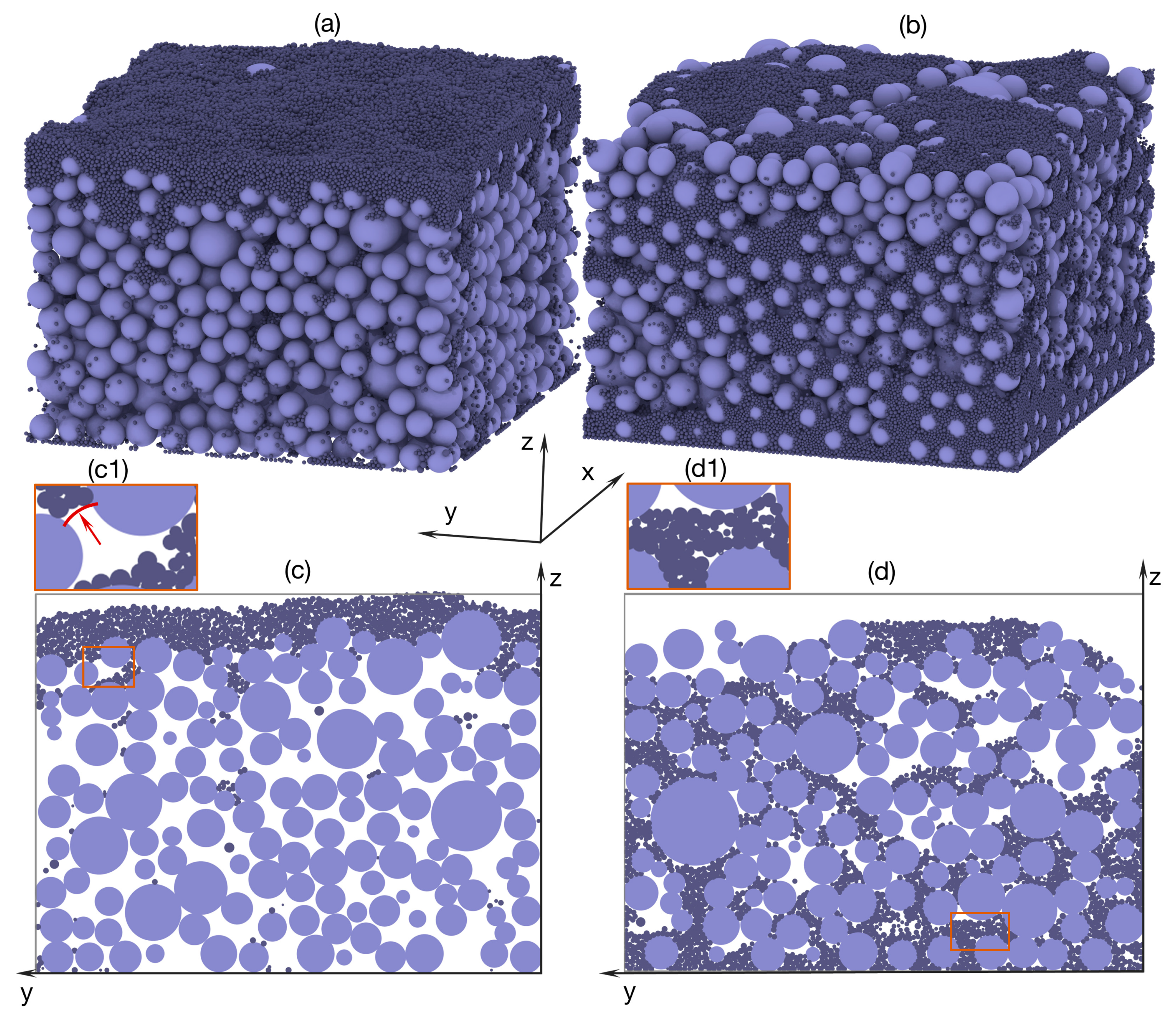
Figure 8 presents the structure of the gravel-bed as well as the distribution of fine sediments for Case-3 and Case-4 at the end of the simulation. Figure 8a shows the 3D structure of the gravel-bed and fine sediment distribution in the bridging case. The infiltration process was stopped when the top gravel layer was filled. Figure 8c shows exemplarily bed materials at the middle x cross-section at the end of the simulation, where the clogging of fine sediment occurs at the surface. The formed fine sediment layer prevented the upper sediment from filling to the sublayer, where almost all void space remained empty. As can be seen in Figure 8(c1), although the diameters of fine particles are significantly smaller than the void space, they connect to build the ‘bridge’ across gravel called ‘cake filtration’, which depends on the size ratio of gravel and the vertical fine sediment rate [43,44,45]. Figure 8b shows the 3D structure of a gravel-bed and fine sediment distribution in the percolation case. The ratio of mean diameter gravel and fine sediment (Dm/dm) in our simulation (52,69) is in the range of percolation (30–70). In this ratio, fine particles are easy to infill to gravel, a fact consistent with what has been found in previous studies [46]. Figure 8d shows the middle x axis cross-section with most of its void space filled by sediment, however, not all void space was entirely filled. In the bottom of the simulation domain (Figure 8(d1)), fine sediment could not move down because of the bottom walls effect, leading to a sudden increase of fine fraction near the flume bed. This phenomenon usually occurred in flume experiments with gravel and fine sediment [10,42,47]. While there are some limitations in the time and scale of the simulations, it can be said that DEM is suitable for simulating the realistic 3D structure of fine sediment and gravel.
Figure 9 shows the comparison between the predicted results of fine sediment distribution and Gibson’s [42] experiments in the bridging and percolation cases. In the top layer-bridging case, the fine sediment fraction reached its highest value (0.6) and values decrease with depth and a final large increase at the bottom. Opposition results found in the percolation case in Figure 9b presents a larger amount of fine sediment that was stored in the sublayer (average fine fraction 0.22) and at the surface layer (average fine fraction 0.19). From the bottom, we can observe a wave-form of fine fraction variation due to bottom wall effect and the interactions between particles. The amplitude of the wave is reduced with the elevation because of the influence of the wall effect, resulting in a reduction in chaotically stacked particles in the upper layer. To evaluate the performance of the model, the correlation coefficient (R), root mean square error (RMSE), and mean absolute error (MAE) are used—details of these equations are introduced in the next part. We reduced the resolution of simulated results from 500 points to 10 points because of the low resolution of the experiment results as well as the collected averaged seven measurements data at six different flume positions (5.5, 7.8, 9.8, 12.5, 16.5, 18.5 m, and ‘the still water’) [42]. It needs to be emphasized that the experiments and measurements have been conducted in a large flume with no sediment transport, while due to high computational requirements, our model only considered a small window, 0.15 m wide and 0.5 m long with quiescent water. There are small differences between our results and measurement data of Reference [42] due to the rescaling of the experiment. However, we obtained a good agreement between the experimental and numerical results (Table 4). The validated results of the DEM method for simulation with fine sediment infiltration into gravel-bed are used to generate data for the FNN model, which is introduced in the next part.

3.4. Input Data for FNN

As mentioned above, we used the results obtained by the DEM for Case-3 and Case-4 to develop FNN models. Furthermore, based on DEM grain mixtures, we create two groups of data namely Data-classification-1 and Data-classification-2 as follow:
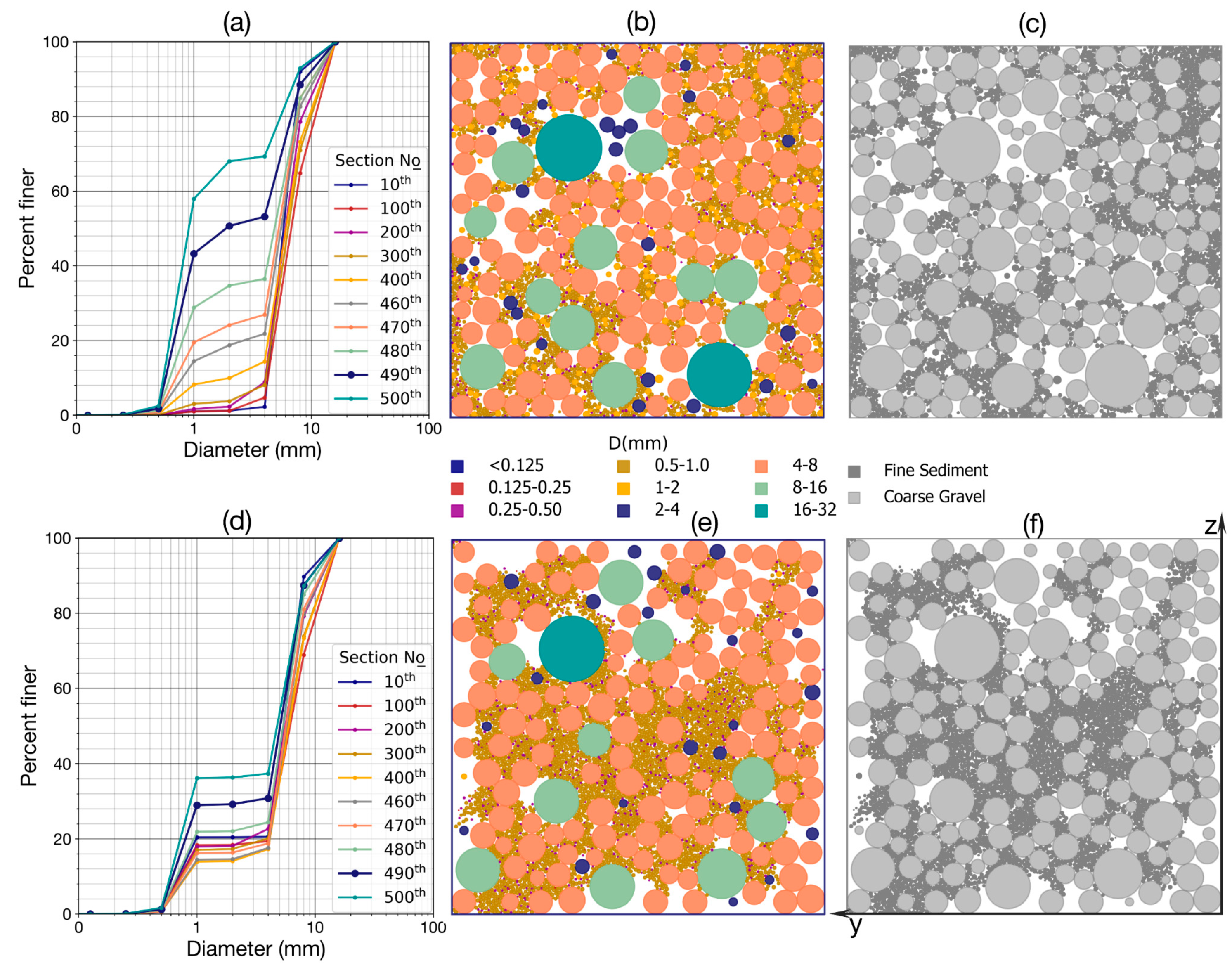
Data-classification-1: The mixture is characterized by 9 grain-sizes, inputs parameters included: location of sample (l), and 9 fractions: f1 (d1 < 0.125 mm), f2 (0.125 mm ≤ d2 < 0.25 mm), f3 (0.25 mm ≤ d3 < 0.5 mm), f4 (0.5 mm ≤ d4 < 1 mm), f5 (1 mm ≤ d5 < 2 mm), f6 (2 mm ≤ d6 < 4 mm), f7 (4 mm ≤ d7 < 8 mm), f8 (8 mm ≤ d8 < 16 mm), and f9 (16 mm ≤ d9).
Data-classification-2: The mixture is characterized by two grain-sizes. Inputs parameters included location of sample (l), fraction of fine grain (with d < 2 mm), and fraction of coarse grain (with D ≥ 2 mm).
Based on the DEM results, grain size distribution and porosity data were generated for 500 different cross sections along the depth (z-direction) and for 800 different cross sections along the flume (x-direction). That means, we created totally 8 datasets: the 1st dataset using Data-classification-1 for bridging case and in z-direction (called Dataset-1), the 2nd dataset using Data-classification-2 for bridging case and in z-direction (called Dataset-2), the 3rd dataset using Data-classification-1 for percolation case and in z-direction (called Dataset-3), the 4th dataset using Data-classification-2 for percolation case and in z-direction (called Dataset-4),the 5th dataset using Data-classification-1 for bridging case and in x-direction (called Dataset-5), the 6th dataset using Data-classification-2 for bridging case and in x-direction (called Dataset-6), the 7th dataset using Data-classification-1 for percolation case and in x-direction (called Dataset-7), and the 8th dataset using Data-classification-2 for percolation case and in x-direction (called Dataset-8). These datasets contain also the information of cross section location.
Each dataset in x-direction is randomly divided into two subsets of data, namely 80% (400 data) for training and 20% (100 data) for testing purposes. Similarly, we randomly split 800 samples in x-direction of each dataset into two subsets: 80% (640 data) for training and 20% (160 data) testing purposes. Figure 10 shows the exemplary cumulative distribution at 10 different cross sections and grain distribution at cross-section 480th in the z-direction.

3.5. Porosity Prediction Based on FNN Model

Porosity depends on pressure and grain size distribution. In our DEM model, the effects of pressure on porosity, the consequence of forces acting on the grain matrix included gravity, buoyancy, grain friction, and contact force were considered. The influence of these factors contributed to the final location of grain obtained from DEM simulations. Grain diameter and the fraction of each size class are used to represent the characteristic of the grain size distribution.
The statistical indices (R, RMSE, and MAE) of the FNN model performance for four porosity predictions in the z-direction (Datasets 1, 2, 3, and 4) are presented in Table 5. In the bridging case, the prediction based on Data-classification-2 (Dataset-2) performed significantly better than Data-classification-1 (Dataset-1). Similarly, in the percolation case, the prediction using Dataset-4 is slightly better than Dataset-3. The prediction for percolation case achieved higher quality of result than the bridging case. It can be explained that in the bridging case, the fine fraction stored in void space of gravel-bed is smaller than in the percolation case. This lead to the prediction model being able to easily capture the effect fine sediment has on porosity output results. Furthermore, in the percolation case, the distinction between the coarse and fine groups is clear because of the large ratio of coarse gravel to fine sediment. As a result, the errors in the predicted results also reached minimum values (RMSE = 0.005753, MAE = 0.003155) from the model using Data-classification-2 of percolation (Dataset-4).
Figure 11 shows the comparison between the FNN based porosity and the data obtained from DEM. In Figure 11a,d, the predicted porosity variation along the depth is compared with porosity based on Dataset-1 and Dataset-2. The dark magenta dotted line represents the DEM based data, where the minimum porosity reaches the value of 0.24 at the surface layer and increases with depth to reach a maximum value 0.6 near the bottom. Near the box bottom, porosity fluctuated widely. Gravel packing created two clear connection areas: a coarse gravel layer with the bottom box and with the upper layer that suddenly increased void spaces seen at z = 0.00 m and z = 0.012 m in Figure 10a,d. This also confirms the problem with laboratory porosity experiments, specifically how the disturbance of packing near the wall of the container causes pores size near the walls to be consistently larger than near the center of the container (also discussed in Reference [48]).
Figure 11b,c,e,f show the performance of the FNN model and the scatter of porosity for the test dataset. As can be seen in Figure 11b, the FNN prediction using Dataset-1 in bridging case overestimated significantly the high peak (0.58, 0.01), (0.47, 0.018), and (0.43, 0.044) in comparison with the DEM based data. A light overestimation also occurs with the FNN prediction based on Dataset-3 in the percolation case (Figure 11d,e). A point worth noting is that both Dataset-1 and Dataset-3 used Data-classification-1 with nine sizes of grains. While, the performance of the FNN model is very good for Dataset-2 and Dataset-4, which are based on Data-classification-2 with two sizes of grains (Figure 11c,f). Overall, as can be seen in Figure 11, FNN models provide good results for porosity prediction. This suggests that the data-driven method based on the grain size distribution is suitable for porosity prediction along the depth in a gravel-bed.
Figure 12 shows the performance of FNN models using four datasets along the horizontal x-direction for bridging and percolation cases in comparison with the DEM based data. The dark magenta dot-dash lines show the DEM based porosity along the horizontal direction. The porosity values changed from 0.37 to 0.51 in the bridging case—upper panel (Figure 12a) and from 0.22 to 0.40 for percolation—lower panel (Figure 12b). The average oscillation amplitude of porosity for these four cases (0.18) near the sidewall varies significantly more than inside the domain (0.06). This can be partly explained because, when the distance is equal to one medium radius (0.007 m) from the wall, the center of coarse particles stack along a vertical plane parallel to the wall, where the highest density of material is reached and reduces with distance from the center of the grain. The effect of the sidewall on the increasing porosity was also discussed in the previous experimental study [41,48,49].
In Figure 12a,b, the FNN prediction based on four Datasets (5, 6, 7, and 8) gave poor results at profiles, x = 0.010 and 0.140 and some other profiles. The model did not agree with the curve of DEM based porosity distribution (e.g., x = 0.095–0.135 m). The model tends to over fit a few points with sudden increases and decreases of fine sediment due to the two sidewalls. Inversely, inside the flume when the porosity did not fluctuate significantly, the model was found to under fit. However, in general, the performances of models are in good agreement with the DEM based data. Table 6 shows relatively good results of porosity prediction and in x-direction, FNNs using Dataset-6, and Dataset-8 perform better than using Dataset-5 and Dataset-7, respectively.
Eight datasets were used to train the FNN networks. Regarding the influence of the grain classifications on the efficiency of FNN models, we observed slight differences between Data-classification-1 and Data-classification-2. As can be seen in the Table 5 and Table 6, the statistical parameters of datasets based on Data-classification-2 are better than datasets based on Data-classification-2. Interestingly, with more detailed classification, the porosity prediction is not as good as in the less detailed classification. This suggest that, with the large size ratio of coarse gravel to fine sediment (D/d greater than 6.4), the detailed classification contained the little information groups (usually the coarse groups with the diameter larger than 2 mm) that may cause some inaccuracies in predicting porosity. This is consistent with the former study conducted by Bui et al. [7] in that the variation of porosity of gravel-bed is mainly caused by the variation in fine sediment rather than the effect of the rearrangement of coarse gravel. The redundancy of usefulness information increased the capability of FNN.
While the time required for training was significantly long (approximation 4 hours for one dataset), we have to train the model only once for each dataset. After the training process, we obtained an explicit relationship between porosity and the inputs, which can then be used to calculate the porosity with other datasets of inputs. Thus, the time needed to calculate porosity is reduced significantly by employing a FNN method in comparison with using sole DEM. It is needed to emphasize that a data-driven method can entirely replace the DEM in calculating porosity. Of cause, this replacement is strictly applied for the same variable range of the grain size distribution. Nonetheless, the reduced simulation time does not only save the computer resources, but also makes the connection between FNN and conventional hydro-morphodynamics model more robust.

4. Conclusions

The void of bed material plays an important role in fluvial geomorphology, exchange processes between river and groundwater and river ecosystem. Thus, predicting the variation of void space in gravel-beds plays a crucial role in eco-hydraulic management and fine sediment budget. In this research, we developed a model framework, which combined Discrete Element Method and Artificial Neural Network for porosity prediction. DEM realistically simulated porosity samples and fine sediment infiltration into 3D gravel-bed structure. An algorithm was developed to extract the simulated DEM results to calculate grain size distribution and porosity. Eight different datasets were generated based on the DEM results and applied to design several Artificial Neural Networks to find the relationship between grain size distribution and porosity. The results demonstrated that the combination of DEM and ANN is successful in simulating porosity and the infiltration process of fine sediment into the gravel-bed.
The validity of the presented model in the case of flowing water and sediment transport has not yet been verified, but it is believed that this model framework has a good performance for the analysis of bed and porosity changes. As a next step, to increase the quality of the training data, the effect that flow velocity has on sediment packing will be considered by coupling with OpenFOAM 5.0.0, open-source computational fluid dynamics (CFD) software, to study fluid-particles interactions. This model concept can be applied to calculate porosity change in a gravel-bed river for bed-porosity variation models as well as to define the exchange rate of fine sediment in gravel-bed rivers.

Author Contributions

V.H.B. designed the study, processed and analyzed the data, developed the models, interpreted the results and wrote the paper. The study has been carried out under the supervision of M.D.B. and P.R., who contributed to the model development stage with theoretical considerations and practical guidance, assisted in the interpretations and integration of the results and helped in preparation of this paper with proof reading and corrections.

Funding

This research was funded by the Vietnam International Education Development (VIED) Scholarship.

Acknowledgments

The contents of this paper are solely the liability of the authors and under no circumstances may be considered as a reflection of the position of the VIED Scholarship. The German Research Foundation (DFG) and the Technical University of Munich (TUM) supported this work in the framework of the Open Access Publishing Program. We much appreciate their help. Special thanks to TUM English Coaching Program for valuable supports and comments to improve this paper. We thank the editor and anonymous reviewers for their constructive comments, which helped us to improve the manuscript.

Conflicts of Interest

The authors declare no potential conflict of interest.

References

  1. Frings, R.M.; Kleinhans, M.G.; Vollmer, S. Discriminating between pore-filling load and bed-structure load: A new porosity-based method, exemplified for the river Rhine. Sedimentology 2008, 55, 1571–1593. [Google Scholar] [CrossRef]
  2. Nunez-Gonzalez, F.; Martin-Vide, J.P.; Kleinhans, M.G. Porosity and size gradation of saturated gravel with percolated fines. Sedimentology 2016, 63, 1209–1232. [Google Scholar] [CrossRef]
  3. Gayraud, S.; Philippe, M. Influence of Bed-Sediment Features on the Interstitial Habitat Available for Macroinvertebrates in 15 French Streams. Int. Rev. Hydrobiol. 2003, 88, 77–93. [Google Scholar] [CrossRef]
  4. Verstraeten, G.; Poesen, J. Variability of dry sediment bulk density between and within retention ponds and its impact on the calculation of sediment yields. Earth Surf. Process. Landf. 2001, 26, 375–394. [Google Scholar] [CrossRef]
  5. Wilcock, P.R. Two-fraction model of initial sediment motion in gravel-bed rivers. Science 1998, 280, 410–412. [Google Scholar] [CrossRef] [PubMed]
  6. Driscoll, F.G. Groundwater and Wells, 2nd ed.; Johnson Filtration Systems Inc.: Saint Paul, MN, USA, 1986. [Google Scholar]
  7. Bui, V.H.; Bui, M.D.; Rutschmann, P. Advanced Numerical Modeling of Sediment Transport in Gravel-Bed Rivers. Water 2019, 11, 550. [Google Scholar] [CrossRef]
  8. Doherty, J. Calibration and Uncertainty Analysis for Complex Environmental Models; Watermark Numerical Computing: Brisbane, Queensland, Australia, 2015. [Google Scholar]
  9. Wu, W.; Wang, S.S. Formulas for sediment porosity and settling velocity. J. Hydraul. Eng. 2006, 132, 858–862. [Google Scholar] [CrossRef]
  10. Wooster, J.K.; Dusterhoff, S.R.; Cui, Y.T.; Sklar, L.S.; Dietrich, W.E.; Malko, M. Sediment supply and relative size distribution effects on fine sediment infiltration into immobile gravels. Water Resour. Res. 2008, 44. [Google Scholar] [CrossRef] [Green Version]
  11. Peronius, N.; Sweeting, T.J. On the correlation of minimum porosity with particle size distribution. Powder Technol. 1985, 42, 113–121. [Google Scholar] [CrossRef]
  12. Carling, R.C.; Templeton, D. The effect of carbachol and isoprenaline on cell division in the exocrine pancreas of the rat. Q. J. Exp. Physiol. 1982, 67, 577–585. [Google Scholar] [CrossRef]
  13. Komura, S. Discussion of “Sediment transportation mechanics: Introduction and properties of sediment”. J. Hydraul. Div. 1963, 89, 263–266. [Google Scholar]
  14. Frings, R.M.; Schuttrumpf, H.; Vollmer, S. Verification of porosity predictors for fluvial sand-gravel deposits. Water Resour. Res. 2011, 47. [Google Scholar] [CrossRef]
  15. Ouchiyama, N.; Tanaka, T. Porosity estimation for random packings of spherical particles. Ind. Eng. Chem. Fundam. 1984, 23, 490–493. [Google Scholar] [CrossRef]
  16. Yu, A.B.; Standish, N. Estimation of the Porosity of Particle Mixtures by a Linear-Mixture Packing Model. Ind. Eng. Chem. Res. 1991, 30, 1372–1385. [Google Scholar] [CrossRef]
  17. Yu, A.B.; Standish, N. Limitation of Proposed Mathematical-Models for the Porosity Estimation of Nonspherical Particle Mixtures. Ind. Eng. Chem. Res. 1993, 32, 2179–2182. [Google Scholar] [CrossRef]
  18. Suzuki, M.; Oshima, T. Estimation of the co-ordination number in a multi-component mixture of spheres. Powder Technol. 1983, 35, 159–166. [Google Scholar] [CrossRef]
  19. Nolan, G.; Kavanagh, P.E. Computer simulation of random packings of spheres with log-normaldistributions. Powder Technol. 1993, 76, 309–316. [Google Scholar] [CrossRef]
  20. Desmond, K.W.; Weeks, E.R. Influence of particle size distribution on random close packing of spheres. Phys. Rev. E 2014, 90, 022204. [Google Scholar] [CrossRef] [Green Version]
  21. Saljooghi, B.S.; Hezarkhani, A. Comparison of WAVENET and ANN for predicting the porosity obtained from well log data. J. Pet. Sci. Eng. 2014, 123, 172–182. [Google Scholar] [CrossRef]
  22. Bui, M.D.; Kaveh, K.; Rutschmann, P. Integrating Artificial Neural Networks into Hydromorphological Model for Fluvial Channels. In Proceedings of the 36th IAHR World Congress, Hague, The Netherlands, 28 June–3 July 2015; pp. 1673–1680. [Google Scholar]
  23. Link, C.A.; Himmer, P.A. Oil reservoir porosity prediction using a neural network ensemble approach. In Geophysical Applications of Artificial Neural Networks and Fuzzy Logic; Springer: Berlin/Heidelberg, Germany, 2003; pp. 197–213. [Google Scholar]
  24. Bagheripour, P.; Asoodeh, M. Fuzzy ruling between core porosity and petrophysical logs: Subtractive clustering vs. genetic algorithm-pattern search. J. Appl. Geophys. 2013, 99, 35–41. [Google Scholar] [CrossRef]
  25. Kraipeerapun, P.; Fung, C.C.; Nakkrasae, S. Porosity prediction using bagging of complementary neural networks. In Proceedings of the International Symposium on Neural Networks; Springer: Berlin/Heidelberg, Germany, 2009; pp. 175–184. [Google Scholar]
  26. Toro-Escobar, C.M.; Parker, G.; Paola, C. Transfer function for the deposition of poorly sorted gravel in response to streambed aggradation. J. Hydraul. Res. 1996, 34, 35–53. [Google Scholar] [CrossRef]
  27. Cundall, P.A.; Strack, O.D. A discrete numerical model for granular assemblies. Geotechnique 1979, 29, 47–65. [Google Scholar] [CrossRef]
  28. Johnson, K.L. Contact Mechanics; Cambridge University Press: Cambridge, UK, 1985. [Google Scholar]
  29. Fleischmann, J.; Serban, R.; Negrut, D.; Jayakumar, P. On the Importance of Displacement History in Soft-Body Contact Models. J. Comput. Nonlinear Dyn. 2016, 11, 044502. [Google Scholar] [CrossRef]
  30. Landau, L.; Lifshitz, E. Theory of Elasticity, 3rd ed.; Pergamon Press: Oxford, UK, 1986. [Google Scholar]
  31. Mindlin, R. Compliance of elastic bodies in contact. J. Appl. Mech. Trans. ASME 1949, 16, 259–268. [Google Scholar]
  32. Zell, A. Simulation Neuronaler Netze; Addison-Wesley: Bonn, Germany, 1994; Volume 1. [Google Scholar]
  33. Haykin, S. Neural Networks: A Comprehensive Foundation; Prentice Hall: Upper Saddle River, NJ, USA, 1999. [Google Scholar]
  34. Bhattacharya, B.; Price, R.; Solomatine, D.P. Machine learning approach to modeling sediment transport. J. Hydraul. Eng. 2007, 133, 440–450. [Google Scholar] [CrossRef]
  35. Kingma, D.P.; Ba, J. Adam: A method for stochastic optimization. In Proceedings of the 3rd International Conference for Learning Representations, San Diego, CA, USA, 7–9 May 2015. [Google Scholar]
  36. Jangid, M.; Srivastava, S. Handwritten Devanagari Character Recognition Using Layer-Wise Training of Deep Convolutional Neural Networks and Adaptive Gradient Methods. J. Imaging 2018, 4, 41. [Google Scholar] [CrossRef]
  37. He, Z.; Zhang, X.; Cao, Y.; Liu, Z.; Zhang, B.; Wang, X. LiteNet: Lightweight neural network for detecting arrhythmias at resource-constrained mobile devices. Sensors 2018, 18, 1229. [Google Scholar] [CrossRef]
  38. Bui, M.D.; Kaveh, K.; Penz, P.; Rutschmann, P. Contraction scour estimation using data-driven methods. J. Appl. Water Eng. Res. 2015, 3, 143–156. [Google Scholar] [CrossRef]
  39. Heaton, J. Introduction to Neural Networks with Java; Heaton Research, Inc.: St. Louis, MO, USA, 2008. [Google Scholar]
  40. McGeary, R.K. Mechanical packing of spherical particles. J. Am. Ceram. Soc. 1961, 44, 513–522. [Google Scholar] [CrossRef]
  41. Navaratnam, C.U.; Aberle, J.; Daxnerová, J. An Experimental Investigation on Porosity in Gravel Beds. In Free Surface Flows and Transport Processes; Springer: Cham, Switzerland, 2018; pp. 323–334. [Google Scholar]
  42. Gibson, S.; Abraham, D.; Heath, R.; Schoellhamer, D. Vertical gradational variability of fines deposited in a gravel framework. Sedimentology 2009, 56, 661–676. [Google Scholar] [CrossRef]
  43. Gibson, S.; Abraham, D.; Heath, R.; Schoellhamer, D. Bridging Process Threshold for Sediment Infiltrating into a Coarse Substrate. J. Geotech. Geoenviron. Eng. 2010, 136, 402–406. [Google Scholar] [CrossRef]
  44. Holdich, R.G. Fundamentals of Particle Technology; Midland Information Technology and Publishing: Nottingham, UK, 2002. [Google Scholar]
  45. Valdes, J.R.; Santamarina, J.C. Clogging: Bridge formation and vibration-based destabilization. Can. Geotech. J. 2008, 45, 177–184. [Google Scholar] [CrossRef]
  46. Leonardson, R. Exchange of Fine Sediments with Gravel Riverbeds. Ph.D. Thesis, University of California, Berkeley, CA, USA, 2010. [Google Scholar]
  47. Seal, R.; Parker, G.; Paola, C.; Mullenbach, B. Laboratory experiments on downstream fining of gravel, narrow channel runs 1 through 3: Supplemental methods and data. In External Memo M-239; St. Anthony Falls Hydraulic Lab, University of Minnesota: Minneapolis, MN, USA, 1995. [Google Scholar]
  48. Ridgway, K.; Tarbuck, K. Voidage fluctuations in randomly-packed beds of spheres adjacent to a containing wall. Chem. Eng. Sci. 1968, 23, 1147–1155. [Google Scholar] [CrossRef]
  49. Sulaiman, M.; Tsutsumi, D.; Fujita, M. Porosity of sediment mixtures with different type of grain size distribution. Annu. J. Hydraul. Eng. 2007, 51, 133–138. [Google Scholar] [CrossRef]
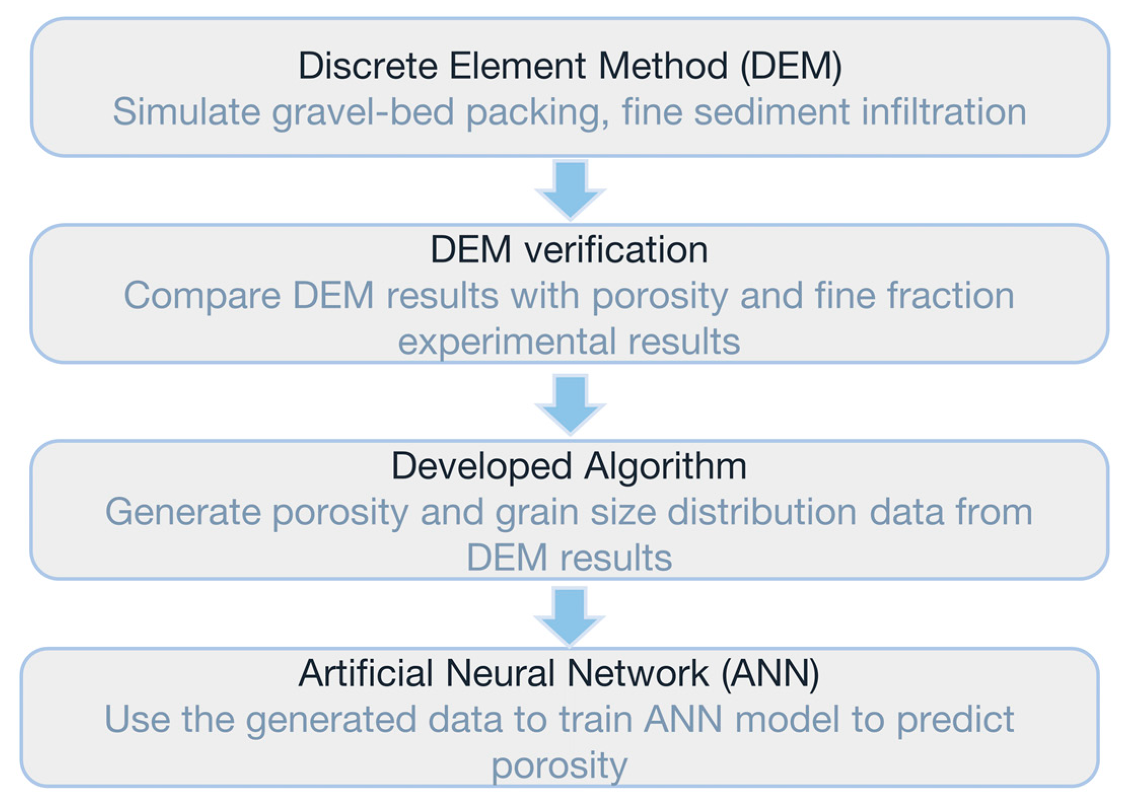
Figure 1. Schematization of porosity estimation using DEM and ANN.
Water 11 01461 g001
Figure 2. Contact forces revised from Fleischmann [29].
Water 11 01461 g002
Figure 3. Calculation sequence within a DEM time step.
Water 11 01461 g003
Figure 4. Calculation parameters of generated circle by k-plane across grain matrix.
Water 11 01461 g004
Figure 5. Three-layer feed forward neural network (a) where input layer has p input nodes, hidden layer has h activation functions, and output layer has q nodes. (b) a node of the network.
Water 11 01461 g005
Figure 6. Porosity of packing of binary mixtures of spheres with size ratio (d/D) 0.14 in comparison with McGeary’s measurement [40] (a) pure coarse grain, (b) fine sediment fraction 0.4, and (c) porosity of mixture.
Water 11 01461 g006
Figure 7. Porosity obtained from DEM simulations in comparison with the porosity measurement of Navaratnam et at. [41] (a) gravel flume, (b) vertical porosity variation.
Water 11 01461 g007
Figure 8. Bed structure of filled gravel at final computational time step. (a) bridging and (b) percolation and of the middle x-axis cross-section, (c) bridging and (d) percolation.
Water 11 01461 g008
Figure 9. Simulated fine fraction variation by the depth in comparison with Gibson measurement [42]. (a) Bridging and (b) percolation.
Water 11 01461 g009
Figure 10. The cumulative grain-size distributions of bed materials at ten different represented cross-sections in z-direction (a) bridging, (d) percolation and bed structures at cross section 480th in z-direction, (b) Dataset-1, (c) Dataset-2, (e) Dataset-3, and (f) Dataset-4.
Water 11 01461 g010
Figure 11. FNN predicted porosity along the depth (z-direction) (a) Datasets 1 and 2, (d) Datasets 3 and 4, and scatter plot (b) Dataset-1, (c) Dataset-2, (e) Dataset-3, and (f) Dataset-4.
Water 11 01461 g011
Figure 12. FNN predicted porosity along x-directio (a) Datasets 5 and 6, (b) Datasets 7 and 8, and Scatter plots (c) Dataset-5, (d) Dataset-6, (e) Dataset-7, and (f) Dataset-8.
Water 11 01461 g012
Table 1. Parameters for numerical simulation.
Density of Sphere (kg/m3)Density of Water (kg/m3)Young’s Modulus (Pa)Poisson RatioFriction between GrainsCoefficient of Restitution
235010005.0 × 1060.450.350.40
Table 2. Statistical performance of porosity simulation using DEM.
Statistical IndicatorsCase-1Case-2
Run 1Run 2
R0.98570.9575260.908266
RMSE0.01650.0485850.059763
MAE0.01250.0361980.05138
Table 3. Time consuming each process for two cases of infiltration process.
ProcessPair TimeNeigh TimeComm TimeOutpt TimeOther Time
Case-3 (Bridging)
Insert14,607.716,269.919.43138.314242593.69
Settle8319.462372.55.847654.092491035.83
Case-4 (Percolation)
Insert24,954.643,270.442.05928.56565287.41
Settle14,112.212,281.211.6083.281252083.9
Pair time: Time to find contact overlaps, forces; Neigh time: Time to form verlet lists, sorting them and finding the neighbors; Comm time: Message Passing Interface (MPI) communication time; Outpt time: Dump and thermo commands; Other time: Other fixes.
Table 4. Verification of Fine Sediment Distribution with Gibson’s Measurement [42].
Statistical IndicatorsCase-3 (Bridging)Case-4 (Percolation)
R0.9691910.940474
RMSE0.1280670.261443
MAE0.0667650.121255
Table 5. Statistical performances of FNN model (for testing data) along the depth (z-direction).
Statistical IndicatorsBridgingPercolation
Dataset-1Dataset-2Dataset-3Dataset-4
R0.9659680.9892060.9908410.994024
RMSE0.0157360.0087860.0078070.005753
MAE0.0095800.0065480.0048980.003155
Table 6. Statistical performances of FNN model (for testing data) along the flume (x-direction).
Statistical IndicatorsBridgingPercolation
Dataset-5Dataset-6Dataset-7Dataset-8
R0.92980.97860.92360.9748
RMSE0.01130.00630.00970.0060
MAE0.00800.00500.00560.0041