1. Introduction
A branching channel or bifurcation is defined as a node where the water flow is divided from a single channel into multiple channels [
1]. Branching channels can exist in many forms, such as braided rivers, alluvial fans, and deltas. These forms result from the hydro-morphodynamic processes of the river [
1,
2]. Man-made branching channels are widely used in irrigation networks, municipal water supplies, and hydropower projects [
3]. Studying the flow behaviour in the branching channel and the location of the flow diversion is essential for water management [
4] and for morphological management downstream of the diversion [
5]. Early studies focused on hydrodynamic features with rigid boundaries, which meant that the experiments did not include sediment transport and movable beds [
6,
7], but still received attention for their explanations using different parameters and geometric forms [
8,
9,
10,
11]. The main hydrodynamic features are the separation zones, stagnation point, and contraction region. Separation zones occur in areas of water recirculation and low flow velocity [
8,
12]. As a result of the recirculation and low velocities, deposition areas appear in these zones [
13,
14]. These zones cause loss in the capacity of the branching channel and consequently reduce the inflow discharge passing through it. This will affect irrigation networks and threatens municipal water supplies and operation of power plants [
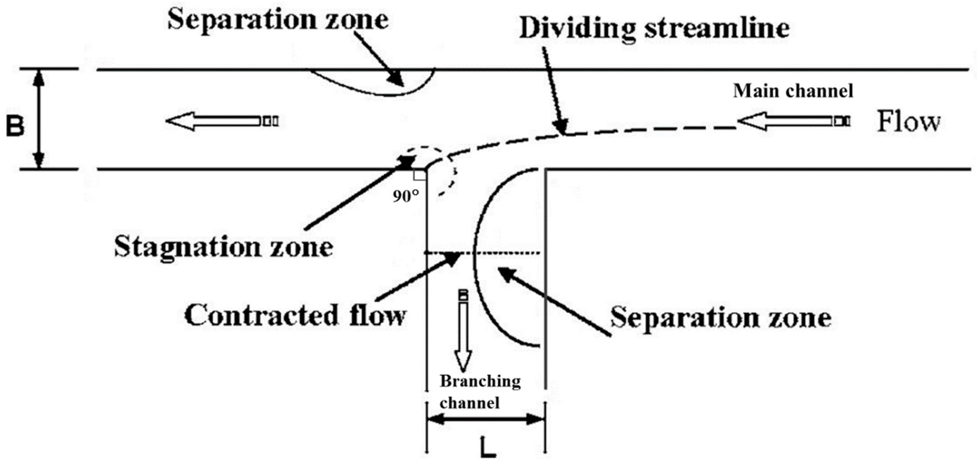
10]. In branching channels, two main separation zones result from the flow, and these zones are shown in
Figure 1.
Separation zone (1) is developed in the branching channel when the flow in the main channel is discharged toward the branching channel. The size and location of the zone (1) are mainly dependent on the discharge ratio and branching angle. An increase in discharge ratio leads to a decrease in the size of the zone (1) [
15]. However, an increase in branching angle from 45° to 90° leads to movement of the separation zone downstream in the branch channel. The smallest separation zone occurred when the branching angle was 30° [
16]. Separation zone (2) is formed near the right bank in the main channel and downstream of the branching junction as shown in
Figure 1. Zone (2) may not form all the time; it usually forms when the discharge in the branching channel takes the major portion of the discharge from the main channel. This flow condition causes the streamlines to curve towards the branching channel where the separation zone expands [
8,
14,
17].
Another hydrodynamic feature found at the corner downstream of the junction is a stagnation point in which the highest pressure and flow depth are found [
8]. The flow contraction zone is formed, owing to the flow separation zone at the beginning of the branching channel. This zone is usually associated with high velocity due to the flow contracted by the separation zone (1). Ramamurthy et al. [
18] found a linear relationship between the contraction area and the discharge ratio (the area increases with the increase in discharge ratio). Lama et al. [
19] found that the contraction flow width at the bottom of the zone is wider than at the surface.
Two important aspects can be summarised from the morpho-dynamic features, and erosion and deposition zones resulted from the nonuniform sediment movements in the diversion channel. In an early experiment, Bulle [
20] recognised sedimentation problems at the branching channel and found that diversion angle, the roundness of the edge of the upstream corner of the diversion, and width ratio between the main and branching channels influence the branching channel behaviour according to the distributions of water and sediment discharge. This had been confirmed by other experimental studies [
21,
22]. Barkdoll et al. [
13] and Herrero et al. [
23] observed a scour hole in the main and diversion channel beds at the downstream junction when the diversion angle was 90°. This scour hole was produced by secondary vortexes created in the junction region. These vortexes played a major role in changing the bed morphology in the main and diversion channels. Alomari et al. [
16] designated that the branching angle should be decreased as much as possible to decrease the scour depth. They conducted experiments with different diversion angles (30°, 45°, 60°, 75°, and 90°) and observed that the minimum scour depth was associated with a diversion angle of 30°.
Studies on controlling morphological features at the junction region used submerged vanes. These studies tried to manage the movement of sediment accumulation at the branching channel section. Submerged vanes are considered one of the most common ways used to control sediment transport at a branching channel [
24,
25,
26,
27]. These submerged vanes are installed in front of the branching channel in the form of rows which created a scour trench [
28] to reduce bed load transport from the main channel to the branching channel. The scour trench traps the sediment from the main channel and redirects it downstream of the main channel [
29,
30]. The size, angle, and number of submerged vanes are considered the most effective parameters in controlling bed sediment movement [
31]. Numerous arrangement schemes of vane rows have been investigated to evaluate their performance in preventing bed sediment transport from entering the branching channel and forming the deposition zone. Barkdoll et al. [
13] investigated two schemes of submerged vane arrangement and found that these vanes could reduce approximately 40% of the branching sediment discharge when the discharge ratio (the percentage of the branching channel discharge relative to the main channel discharge) is >20%. Another different vane arrangement has been tested in different boundary conditions, such as parallel, regular, and zigzag, installed in different numbers of rows with different angles.
Table 1 summarises the several studies that have been conducted experimentally and the practical applications in different sites.
The studies related to the practical application for controlling the sediment that enters the branching channel are those of Wang et al. [
30], Nakata and Ogden [
32], and Michell et al. [
25]. Some limitations and conditions were found in practical cases. For example, Wang et al. [
30] found that the vanes are an effective way for controlling sediment at the branching channel when the flow is small enough, and the velocity at the branching channel is <20% of the main upstream flow velocity. While the other researchers (Nakata and Ogden [
32] and Michell et al. [
25]) combined submerged vanes with other structures such as a skimming or barrier wall to develop a more effective method for controlling sediment movement.
However, we can conclude that the effectiveness of using submerged vanes was limited by flow conditions in which the effective approach had a discharge ratio of up to 20–30%. In some cases, submerged vanes may adversely affect the navigation of the main channel, especially given that these vanes produce a nonuniform velocity distribution near their location [
13]. In addition, submerged vanes are potentially costly because of their number. The limitations of using submerged vanes to control and manage hydro-morphodynamics display the importance of investigating different types of obstacles and approaches. However, in the present study, unsubmerged obstacles, such as vanes, are proposed as control structures to manage the hydro-morphodynamic features in branching channels. In general, the obstacle is used to navigate both flow and bed variations. The hydraulic performance of the obstacle mainly depends on its location, dimensions, and morphological conditions [
37,
38,
39]. For this reason, no specific criteria have been established for designing the obstacle in a channel system. Physical or numerical simulation is needed to optimise the design of the obstacle. However, the use of physical models has some limitations, such as high cost, steady flow, and scale effect. On the other hand, numerical models are low-cost and can be used efficiently for unsteady mobile bed conditions.
Thus, a real branching channel was considered as a case study, in which most of the hydro-morphodynamic features were presented (branching channel in the Tigris River, Iraq). In this site, efforts are made almost annually to remove the sediment accumulation at the separation zone by using a sediment dredging boat. Therefore, studies are needed to find an appropriate method for the management of branching channel systems, especially in urban areas. The significance of this study can be attributed to the simulation of various configurations for controlling deposition and scour zones using vanes and the recommendation of the best solution that provides minimum deposition and scouring zones, while enhancing channel flow dynamics.
2. Materials and Methods
2.1. Study Area and Data Acquisition
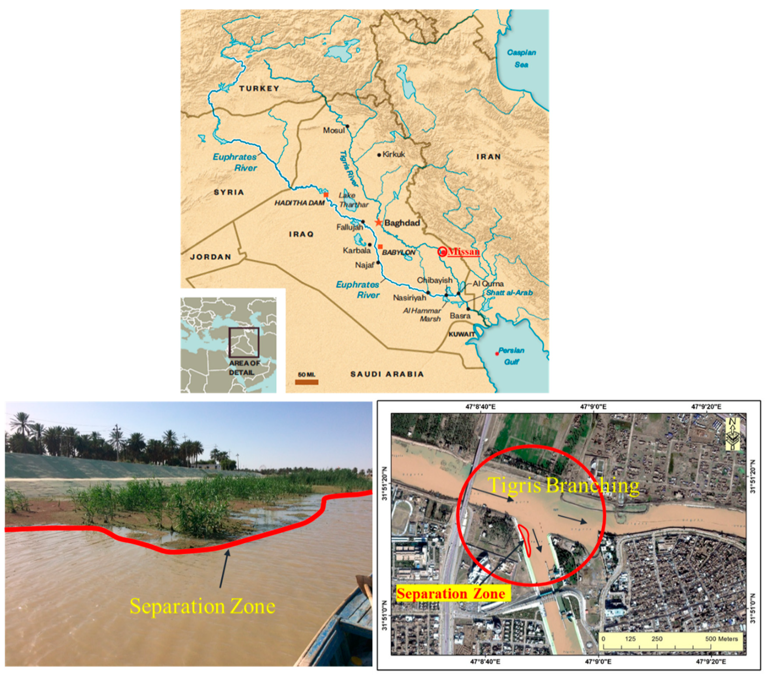
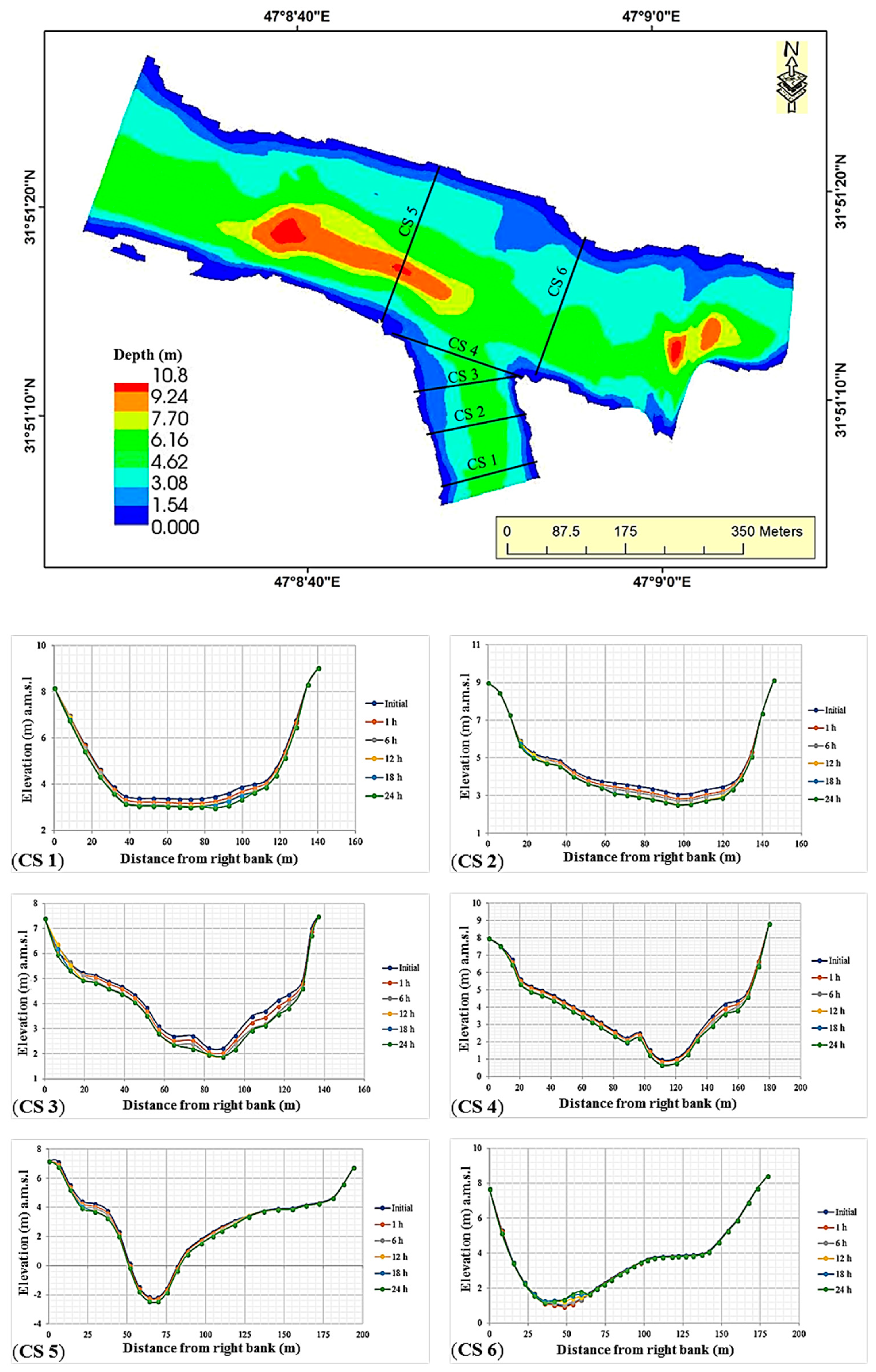
The Tigris branching channel located in the Missan governorate at the southern part of Al-Iraq was chosen as a case study (
Figure 2). The flow in the southern reach of the Tigris River has a significant number of diversion channels, and this branching is considered one of the important junctions in the southern part of the Tigris River system because it is located in the second biggest city in Iraq (Basra city) and many towns depend on its water for municipal and agriculture activities.
Hydro-morphodynamic data of the Tigris branching channel were collected from May to July 2017. Field work included measurements of discharge, velocity, transection geometry (achieved by using the SonTek River Surveyor M9 device), and water levels at various locations in the cross-sections of the main and diversion channels. Bathymetric surveys were conducted using the Garmin echoMap 50s device. For the M9 device, the space between the cross-section was less than 25 m, while for using the echoMap 50s device, the space between the points was around 0.3 m. The slope of the Tigris River at the junction site was measured and found to be 4 cm/km, as it is located in a flat area. The width of the main river is approximately 200 m, while the width of the branching channel is approximately 120 m. The diversion of the branching channel is placed at an angle of 50° from the flow direction of the main Tigris River.
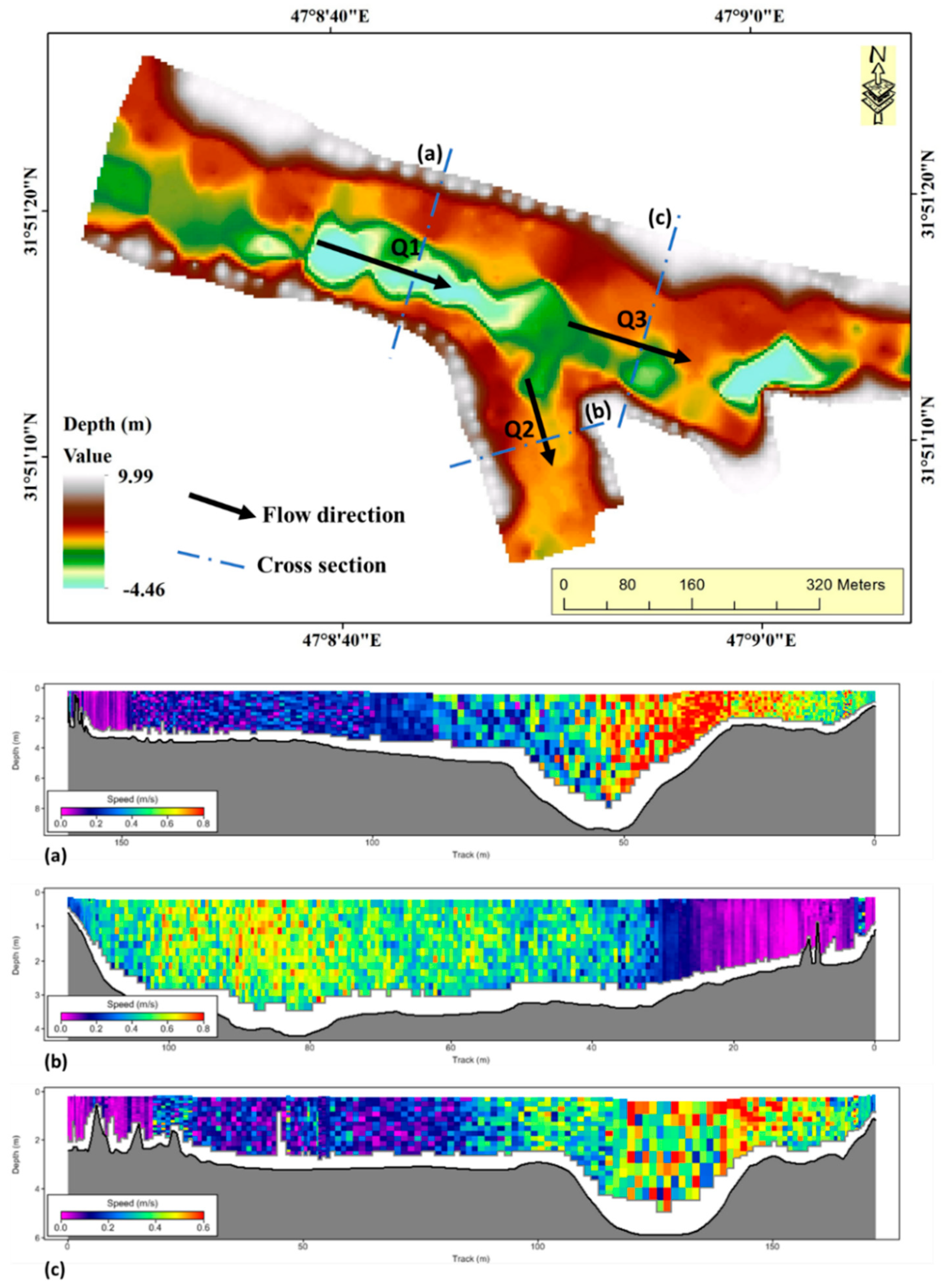
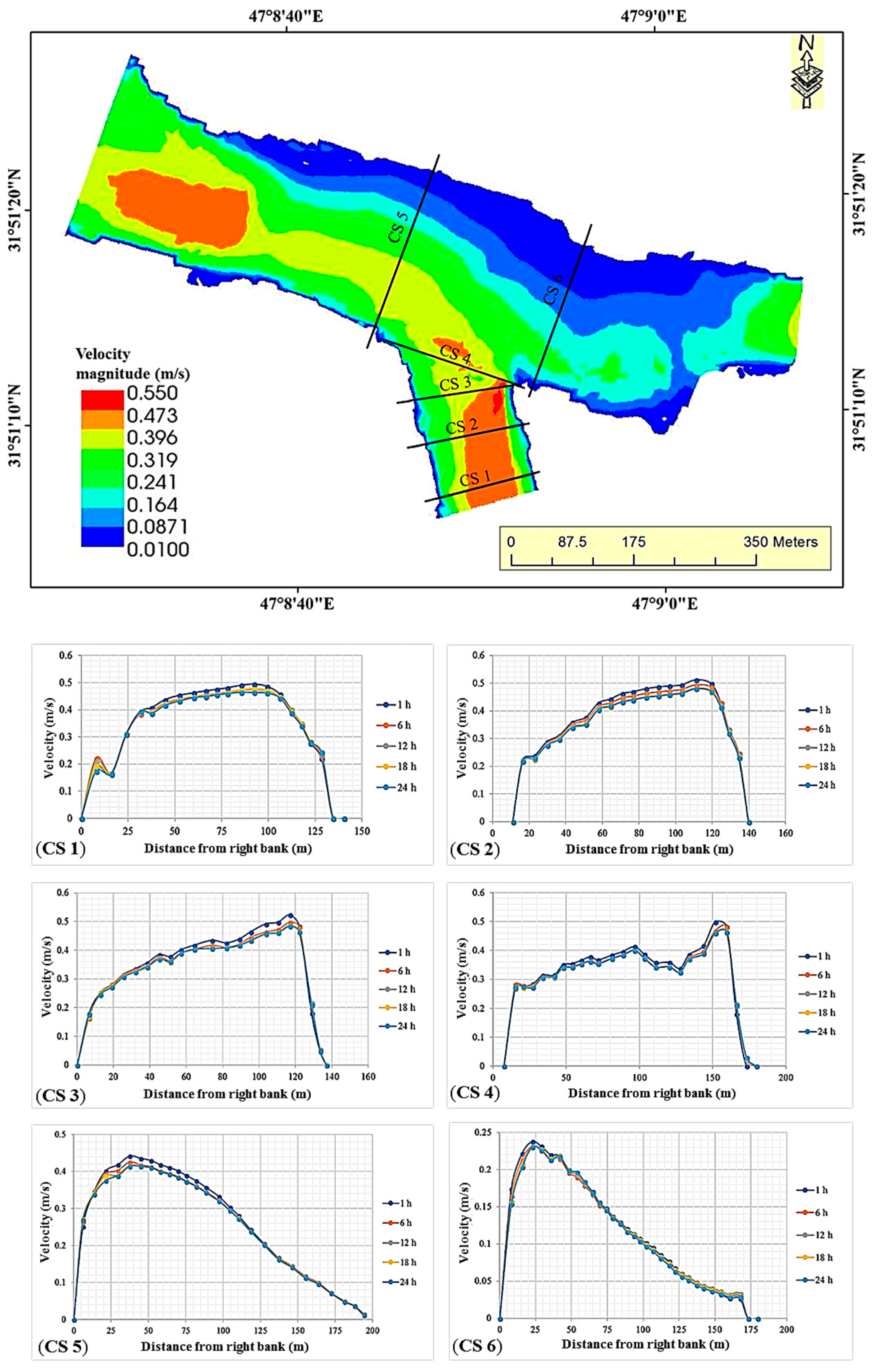
Figure 3 shows the digital elevation map resulting from the measurements of the dense of points at the junction. In addition,
Figure 3 represents the velocity distributions along the cross-sections of the inflow discharge of each reach in the Tigris branching junction. The velocity distributions in the cross-sections are as follow: (a) of Q1 with discharge 247 m
3/s, (b) of Q2 with discharge 127 m
3/s, and (c) of Q3 with discharge 121 m
3/s.
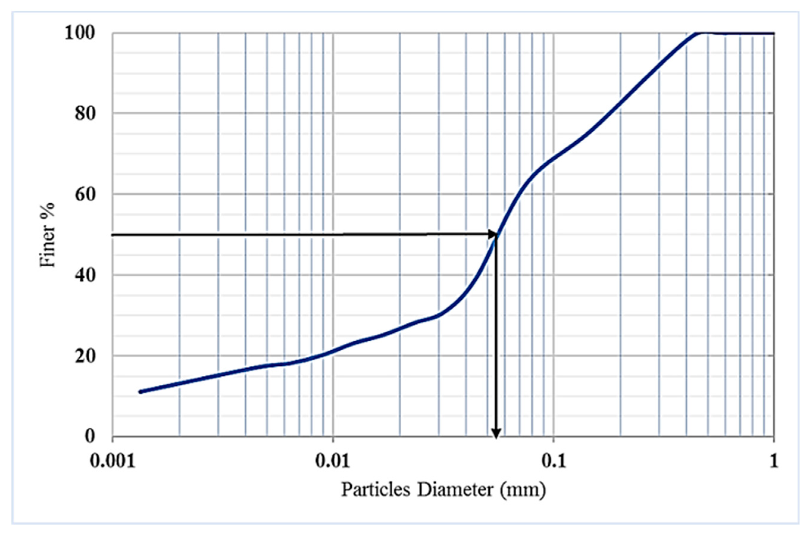
Samples from the riverbed were collected using a van Veen grab sampler to specify the soil type, size, and gradation. The samples of bed material were obtained from 14 points to cover the study area of the branching channel. Two methods are used in the laboratory to determine the characteristics of the particles. First is sieve analysis, which is used to determine the particle size distribution of materials with a diameter of >2 mm. The second method is hydrometer analysis, which is used to determine the particles of soil smaller than sieve no. 200 (0.075 mm). However, in this study, hydrometer analysis was used because most of the particles passed through the sieve. The results from the particle size distribution curves for the Tigris branching channel showed that the average median particle dimeter (d50) was approximately 0.055 mm.
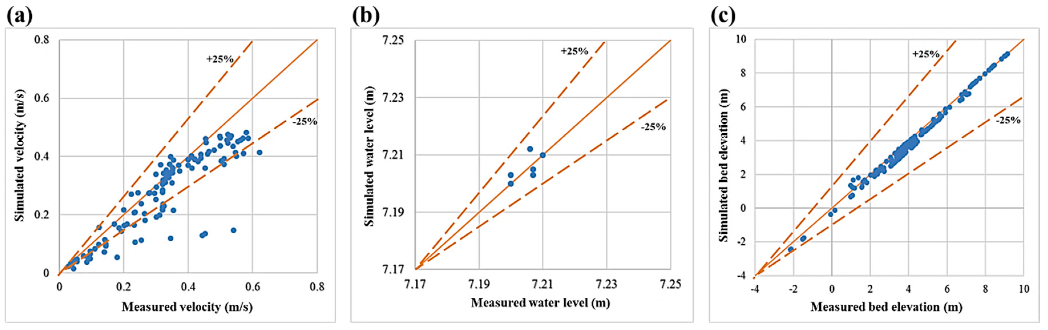
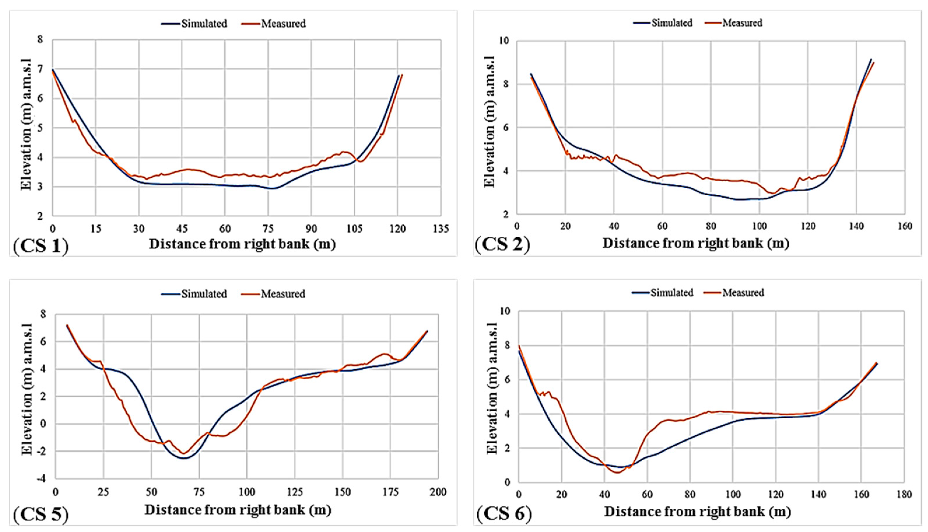
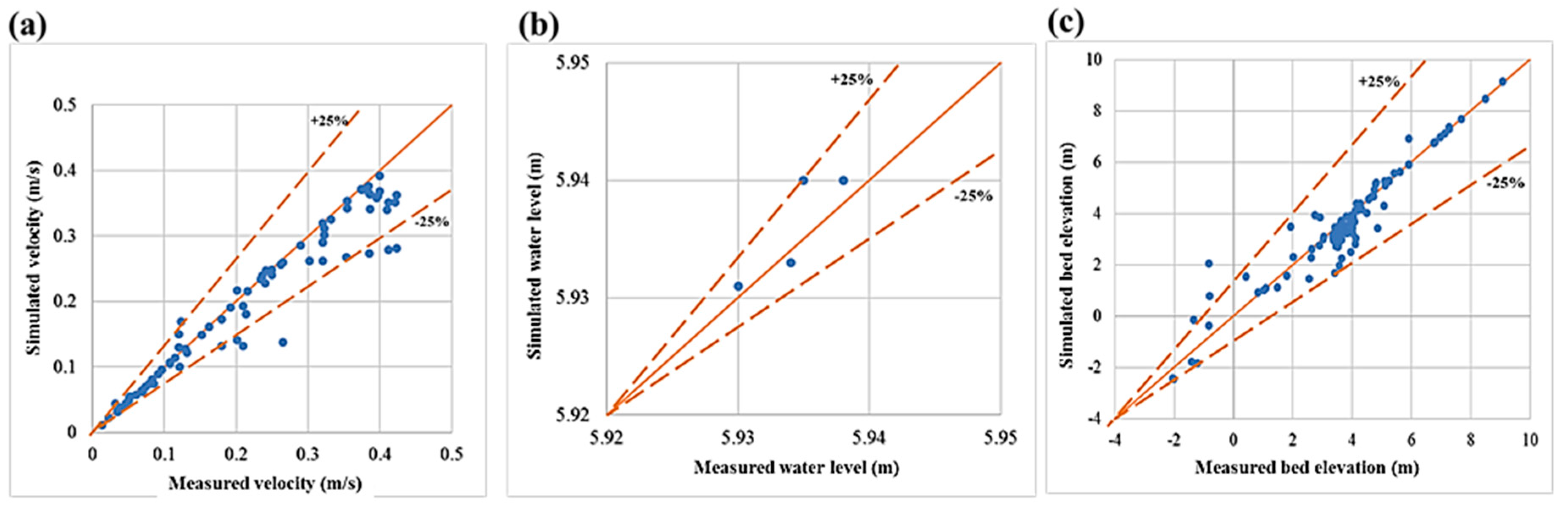
However, the dataset that was measured on 11 May 2017 and included discharge, velocity, water level, cross-section geometry, and bathymetry survey was used to build and calibrate the model, while the dataset measured on 20 July 2017 was used to validate the model.
Table 2 shows the summary of the field data.
2.2. Critical Velocity of the Sediment Inception Motion
The critical shear velocity (
) of the bed material in this study was determined using Shield’s diagram. The dimensionless shear stress (
) expressed in Equation (1) was obtained from the diagram. Critical shear velocity was calculated from Equation (2).
: Critical shear stress of the bed material
: Specific weight of the bed material
: Specific weight of water
: Water density
: Median particle diameter.
By using Shield’s diagram and applying Equations (1) and (2), we obtained a value of 0.013 m/s for the critical shear velocity of the bed material, with a median d50 of 0.055 mm.
For movable bed and sediment transport, knowledge of the threshold point of the sediment particles to be in motion is essential, and most existing studies represent the threshold point of sediment particles in terms of critical mean velocity,
. Many methods can be used for estimating critical mean velocity, of which the Simons and Şentürk method, which is shown in Equation (3), is one of the most common [
16,
40].
: Sediment density.
This equation is frequently adopted to compute the critical mean velocity, and the values range from 0.26 to 0.32 m/s, with low and high water depths (y). Critical velocity is a function of water depth (y), in which the median particle diameter (d50) is known, and the other variables are kept constant for the selected branching of the Tigris River.
2.3. Solver Background, Structure, Characteristics, and Application Procedure
In this study, the solver Mflow_02 was used as a tool to simulate unsteady flow in a selected branching channel of the Tigris River, Iraq. The original version of Mflow_02 was based on the program developed by Tomitokoro et al. [
41] and subjected to improvements. The version made by iRIC [
42] includes additional functions such as a moving boundary model and riverbed variation calculation. This enables the program to calculate 2D plane unsteady flow and riverbed variation by using unstructured meshes of the finite element method in the orthogonal coordinate system (Cartesian coordinate system). The later development enables the model to reproduce the exact structural shape of a complicated landform, particularly in distributaries and confluences. For this reason, the Mflow_02 solver was used to simulate the hydro-morphodynamics of the selected branching channel of the Tigris River in the Missan governorate of Iraq, including the proposed engineering solutions for controlling the scouring and deposition zones. Two main models are embedded in the Mflow_02 solver, namely the flow field and riverbed variation models. These models have many submodels which can help achieve a wide range of calculations.
2.3.1. Flow Field Model
The characteristics of the flow field model are as follows:
A Galerkin finite element submodel (a type of weighted residual method) is used to discretize continuity and momentum equations.
Open boundary conditions (upstream and downstream boundaries, etc.) enable the setting up of various conditions, such as time series of flow discharge, time series of water level, and water level discharge.
The friction of the river bed can be set by using the Manning roughness coefficient. This coefficient can be represented in the model as a polygon for the entire area or for each element (cell), thus providing spatial distribution of roughness.
Three submodels are available for computing the turbulence field (flows with large and small eddies). These are the zero equation submodel, simple k-ε, and direct input of kinematic eddy viscosity. In this study, the zero equation submodel was selected because of its stability in calculating large and small eddies. The kinematic eddy viscosity,
υ, is expressed by using the von Kàrmàn coefficient with
(0.40).
: Bottom friction velocity.
This formula is called the zero equation submodel for turbulence statistics without a transport equation. In flow fields where the water depth and roughness change gradually in the cross-sections of the branching channel, the kinematic eddy viscosity in horizontal and vertical directions is assumed to be in the same order.
Other effects, such as the effect of wind on the water surface and of vegetation on flow, are available in this solver but were disregarded in this study.
2.3.2. Riverbed Variation Model
The characteristics of riverbed variation are as follows:
The riverbed variation associated with the flow field model is calculated. This model can calculate the flow field only or together with riverbed variation.
The riverbed material can be selected from uniform and mixed grain diameters. If a mixed grain diameter is selected, then a variation in grain distribution can be assumed for deep directions and multiple layers.
Three methods for calculating the total bed load
of depth-averaged flow velocity are available in the Mflow_02 solver, and these are the Meyer-Peter and Müller formula [
43], Ashida and Michiue formula [
44] and Engrlund–Hansen formula [
45]. In this study, the Meyer-Peter and Müller formula was adopted for computing the total bed load.
: Gravel density
: Critical tractive force (calculated by the Iwagaki formula, [
46])
: Calculated by Kishi and Kuroki in the formula below [
47].
: Vertical average flow velocity in the flow direction.
The total sediment discharge set by the Meyer-Peter and Müller formula is converted to the normal direction (
n) and tangential direction (
s) of the streamline, in consideration of the effect of secondary flow and riverbed slope, which is caused by streamline curvature of depth-averaged flow velocity [
48].
: (s) direction component of sediment discharge near the riverbed
: (n) direction component of sediment discharge near the riverbed
: Absolute value of velocity near the riverbed
: (s) direction component of flow velocity near the riverbed
: (n) direction component of flow velocity near the riverbed
: Static friction factor
: Kinetic friction factor
: Height of the riverbed.
The scour limit of the riverbed, secondary flow coefficient, and morphological factor can be set accordingly.
Figure 4 shows additional details on the solver’s application.
2.4. Model Implementation and Boundary Conditions
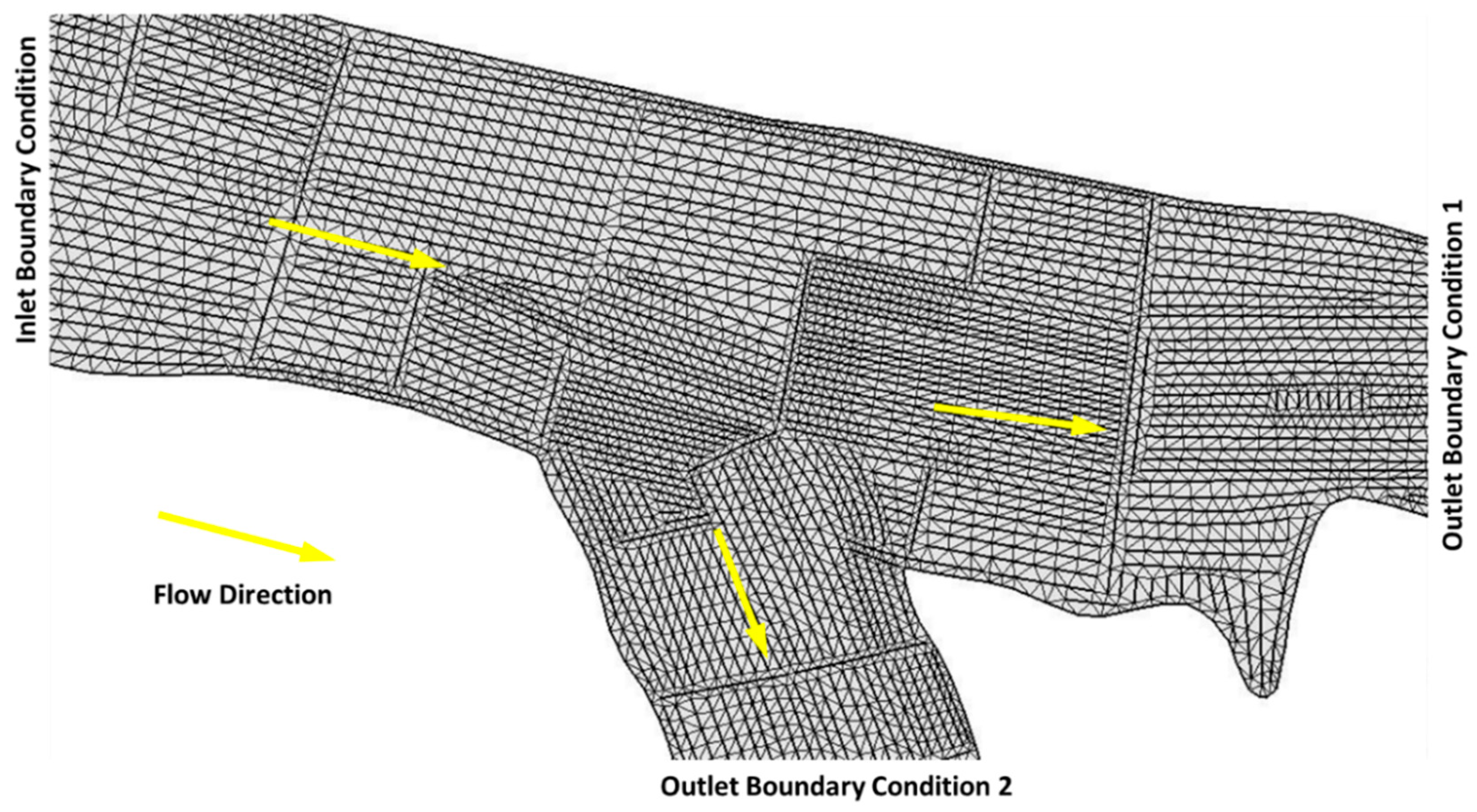
The Mflow_02 model was used to assess morphological changes in the Tigris branching channel. The initial input data were imported from a bathymetry survey for the branching of the Tigris River. A fine unstructured grid consisting of 4511 nodes was created by drawing many lines until good performance was achieved (
Figure 5). A finer grid resolution provides more accurate results, but it needs a small time step (Δ
t). Time step has a direct relationship with the dimension of the grid (
) and velocity (
), which can be expressed as
. In the current model, different time steps were attempted until the hydrodynamic simulation operated smoothly with a time step of 0.04 s. The second input data involved the curves of the grain size distribution of the bed material, in which the average median particles of the Tigris branching channel was approximately 0.055 mm (
Figure 6).
The third input data contained the flow rate at the upstream and the water level at the downstream. A flow rate of 247 m
3/s was set in the inlet boundary condition upstream of the Tigris branching channel. Water levels of 7.205 and 7.2 m above mean sea level were set in outlet boundary conditions 1 and 2, respectively, located downstream of the main and branching channels. Among the turbulence models, a zero-equation model was adopted, and a movable bed computation with a starting time of 800 s was set up to provide stability to the flow field mode operation first and then to the sediment transport and bed deformation. For sediment transport computation, Mflow_02 uses the Ashida and Michiue [
44], Meyer-Peter and Müller [
43], and Engelund–Hansen [
45] equations to compute the total bed load transport. In this study, the Meyer-Peter and Müller equation was selected to compute sediment transport because the equation provides reasonable results for simulated bed elevations. The accuracy of the simulated bed elevations was demonstrated in the calibration and validation results of both models. Other settings related to riverbed morphology and sediment transport were as follows: the scour limit of the riverbed in which the selected branching channel has no limit for scouring was set in the model, the secondary flow coefficient was set to 7 (based on the Engelund model [
45]), and the morphological factor (the ratio of bed deformation to flow) was set to 1. The above-mentioned setting was considered for a real simulation, in which an increase in one of the values leads to an increase in the bed deformation of the branching channel.
2.5. Unsubmerged Vanes as Control Structures
Many types of obstacles have been used in riverine systems to manage and control the training of the rivers. Spur dykes, vanes, groynes, and weirs are among the obstacles used by the US Army Corps of Engineers [
38]. In this study, vanes were used as obstacles to assess the hydro-morphodynamics of the branching channel. This type of structure was introduced in the model by creating a polygon that was excluded throughout the mesh computing and regarded by the model as a nonerodible material [
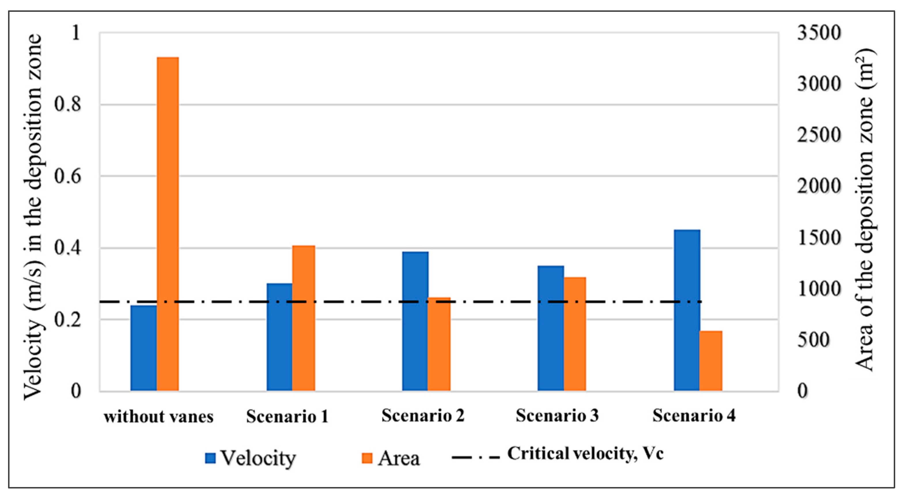
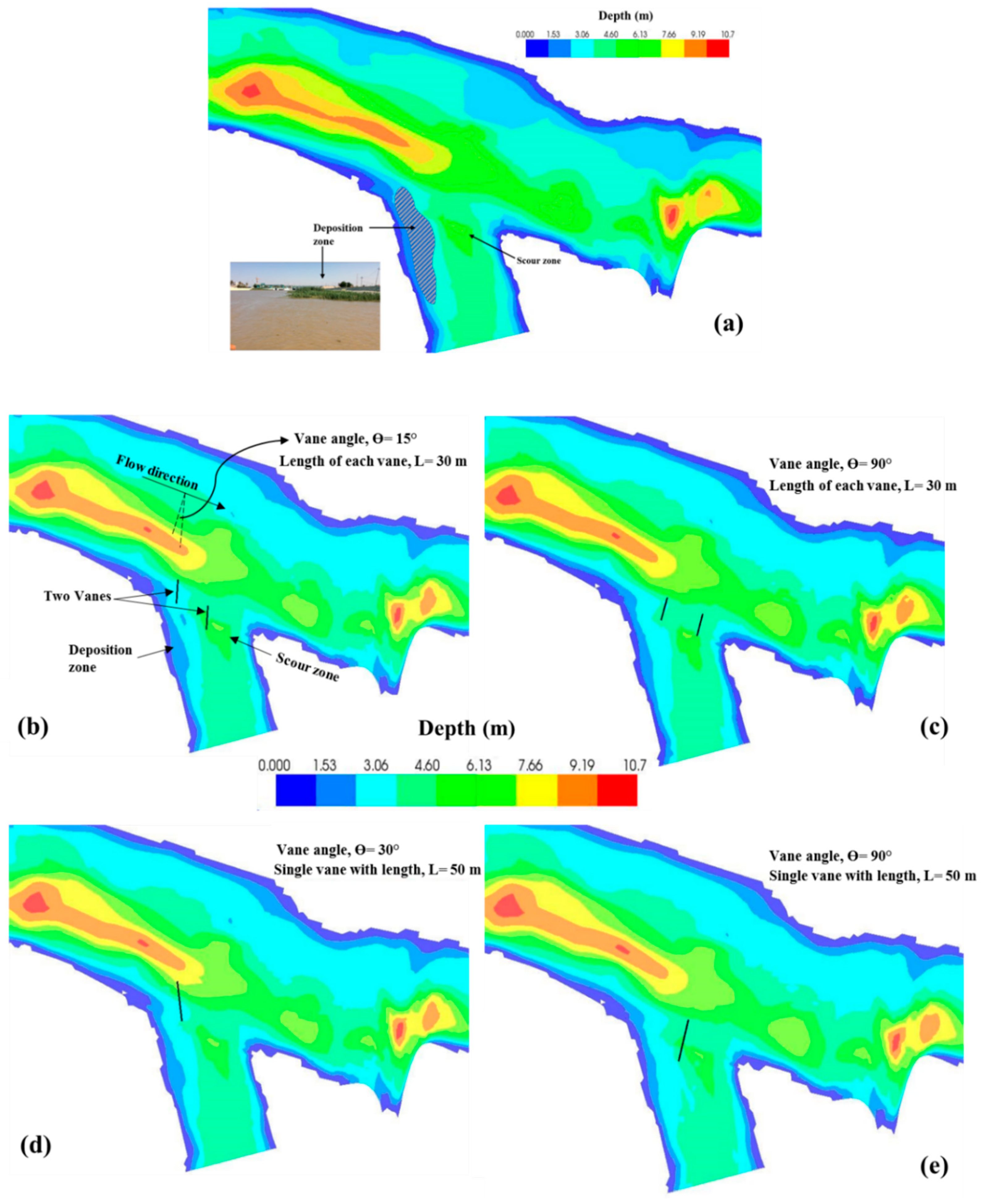
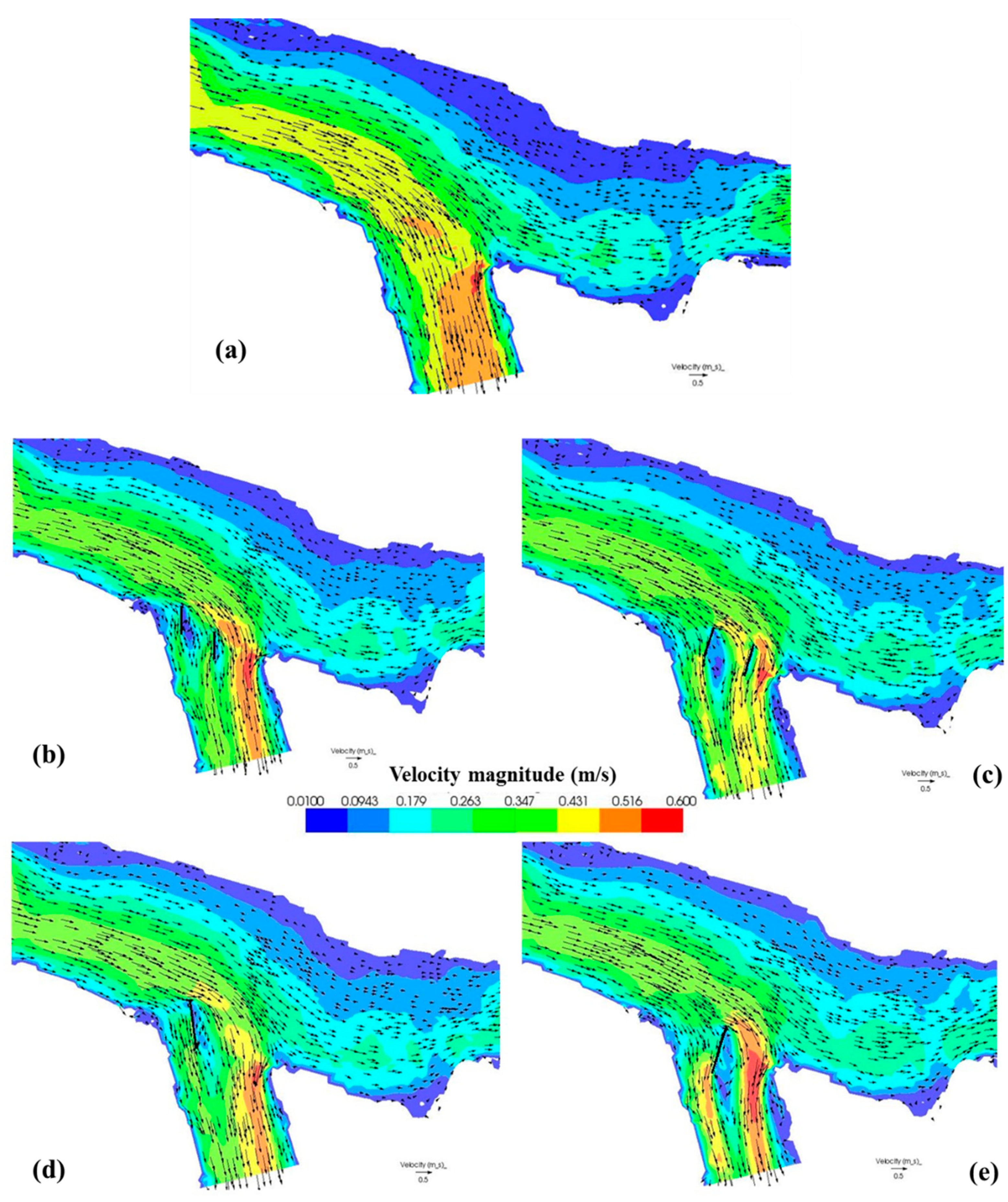
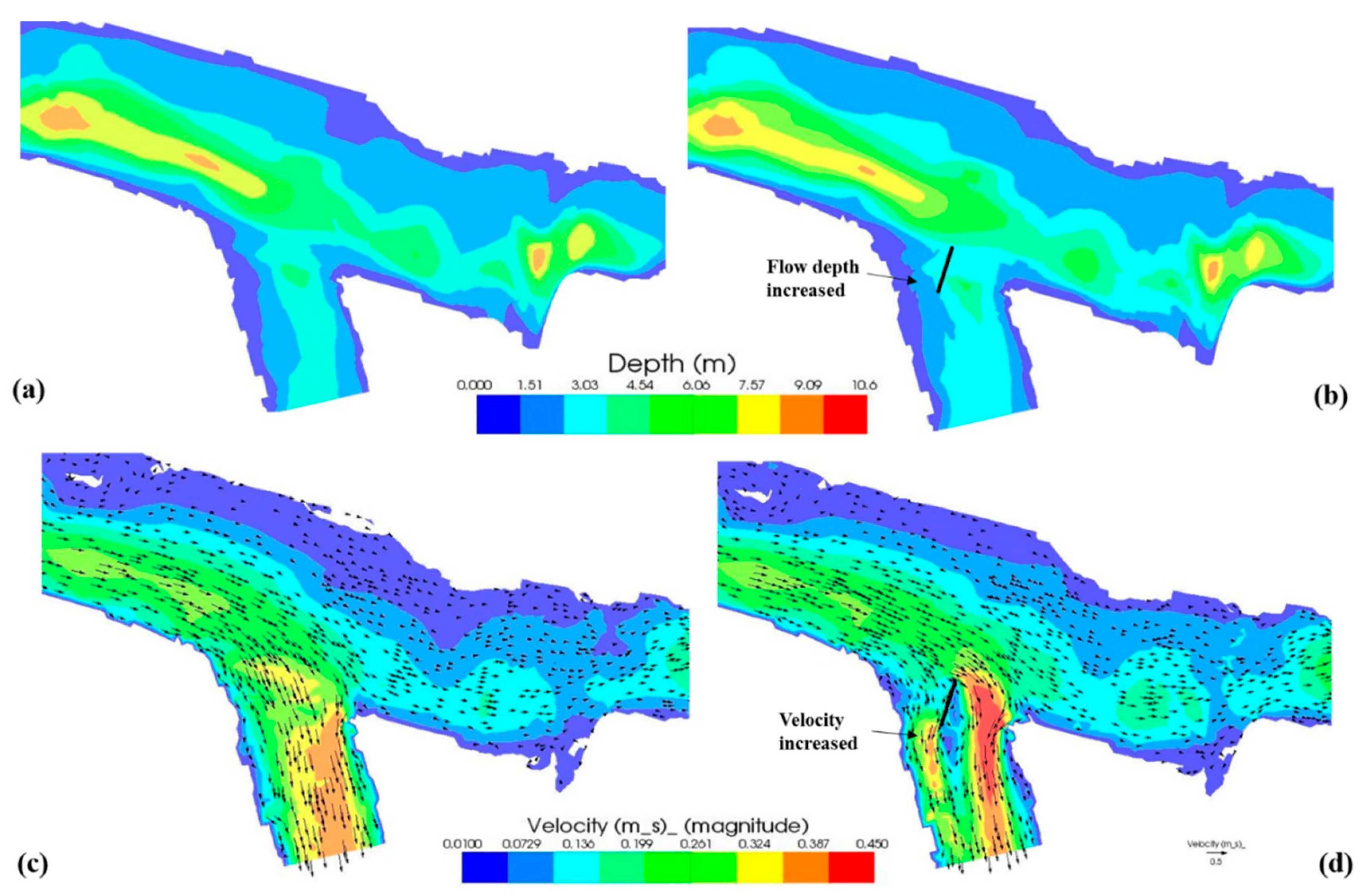
42]. The impact of the following four configurations on the flow in a branching of the Tigris River was clearly shown in the computations of riverbed variation and velocity distribution with the development, appearance, and movement of the sandbar.
Two vanes 30 m long and an inclination angle of 15° from the axis perpendicular to the flow of the main river
Two vanes 30 m long perpendicular to the direction of the flow of the main river
A single vane 50 m long with an inclination angle of 30° from the axis perpendicular to the flow of the main river
A single vane 50 m long perpendicular to the direction of the flow of the main river.
2.6. Statistical Indices
Four statistical indices were used to assess the accuracy of the prediction of the Mflow_02 model, and these were mean absolute deviation (MAD), mean square error (MSE), root mean square error (RMSE), and mean absolute percentage error (MAPE). The criterion for using these methods is to determine the accuracy of the simulation, in which a low statistical value between measured and predicted values indicates high accuracy of simulation performance. These methods can be described by the following equations.
: Amount of data used
M: Measured value
S: Simulated value.

 ,
, 


