Estimating Peak Daily Water Demand under Different Climate Change and Vacation Scenarios


Abstract
:1. Introduction
2. Materials and Methods
2.1. Model Setup
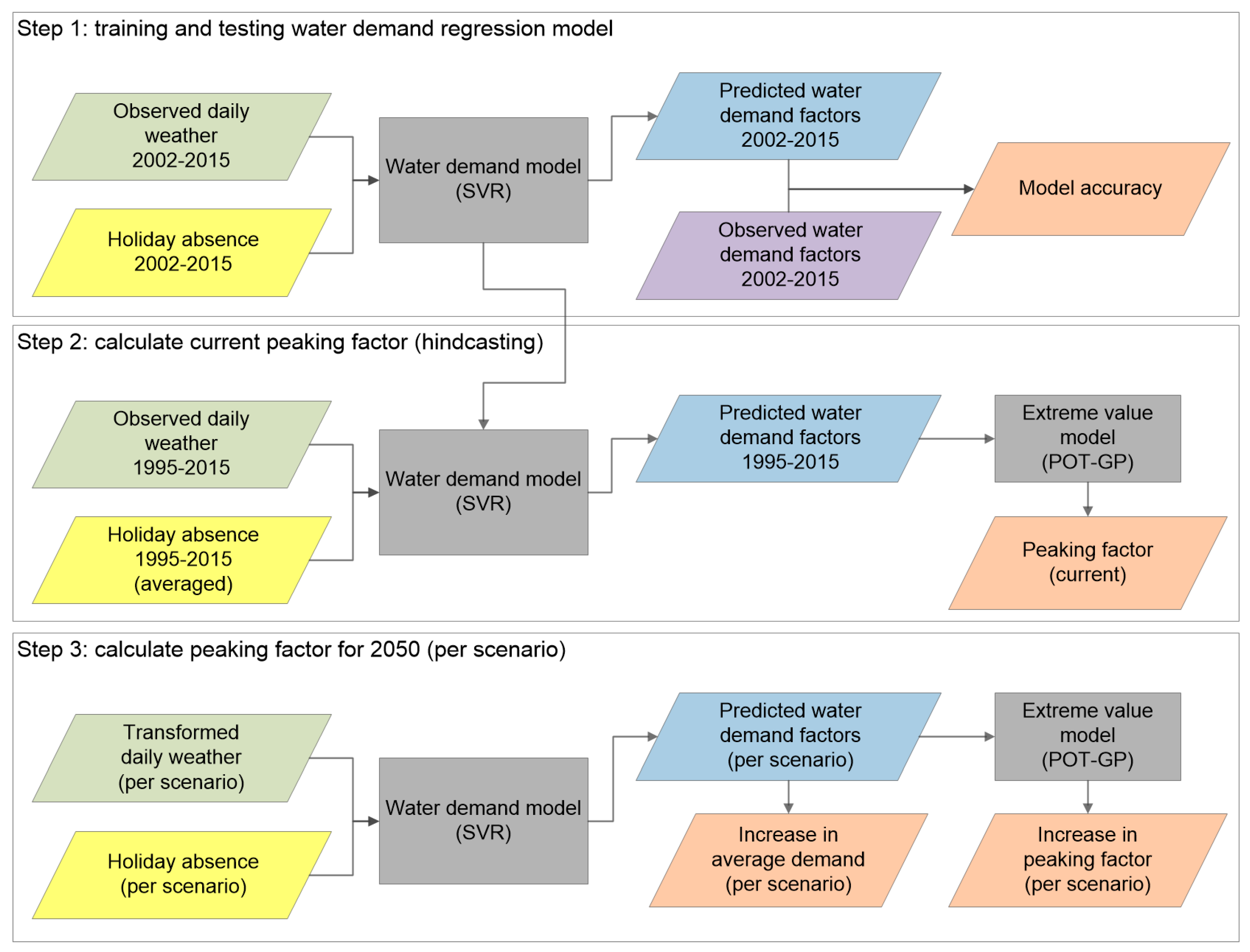
- Train and test a regression model that relates daily weather, vacation-related absence/presence and occurrence of national holidays to the measured drinking water demand. After initial training on observed (historical) drinking water demands, this model can be fed with climate-transformed weather patterns and different vacation scenarios in order to simulate corresponding water demand.
- Apply the regression model to a longer historical period to get homogeneous water demand time series representative for the current climate (hindcasting). Then use an extreme value model that samples peaks from the simulated water demand time series and fits those peaks to a statistical extreme value distribution. From this model the water demand factor corresponding with once in ten years occurrence can be extracted: The peaking factor.
- Finally, develop future scenarios (for horizon 2050 in our case) and use those to generate input time series for the regression model. Apply the regression and extreme value model on input time series for each scenario to obtain future peaking factors.
2.1.1. Regression Model
2.1.2. Extreme Value Model
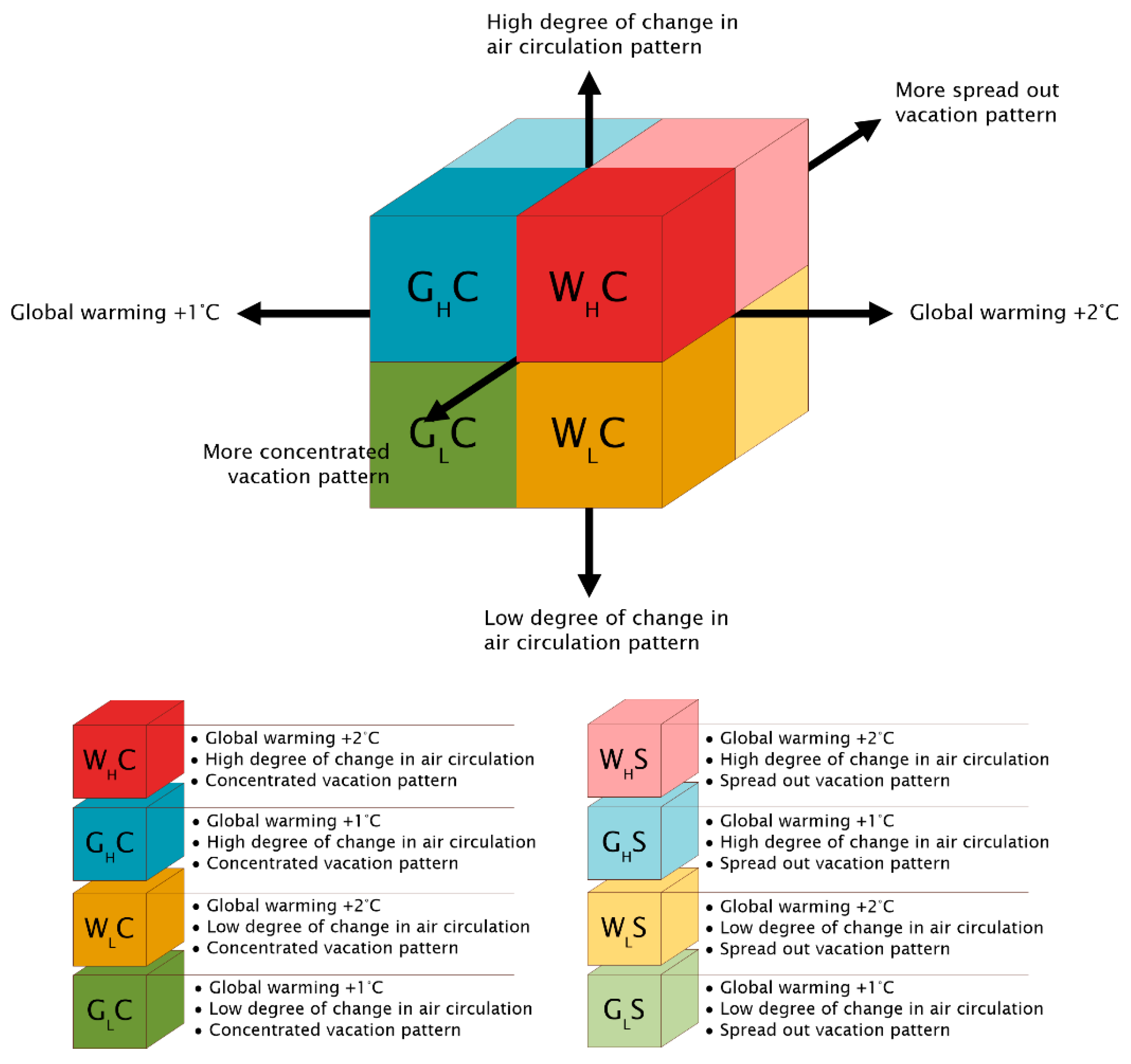
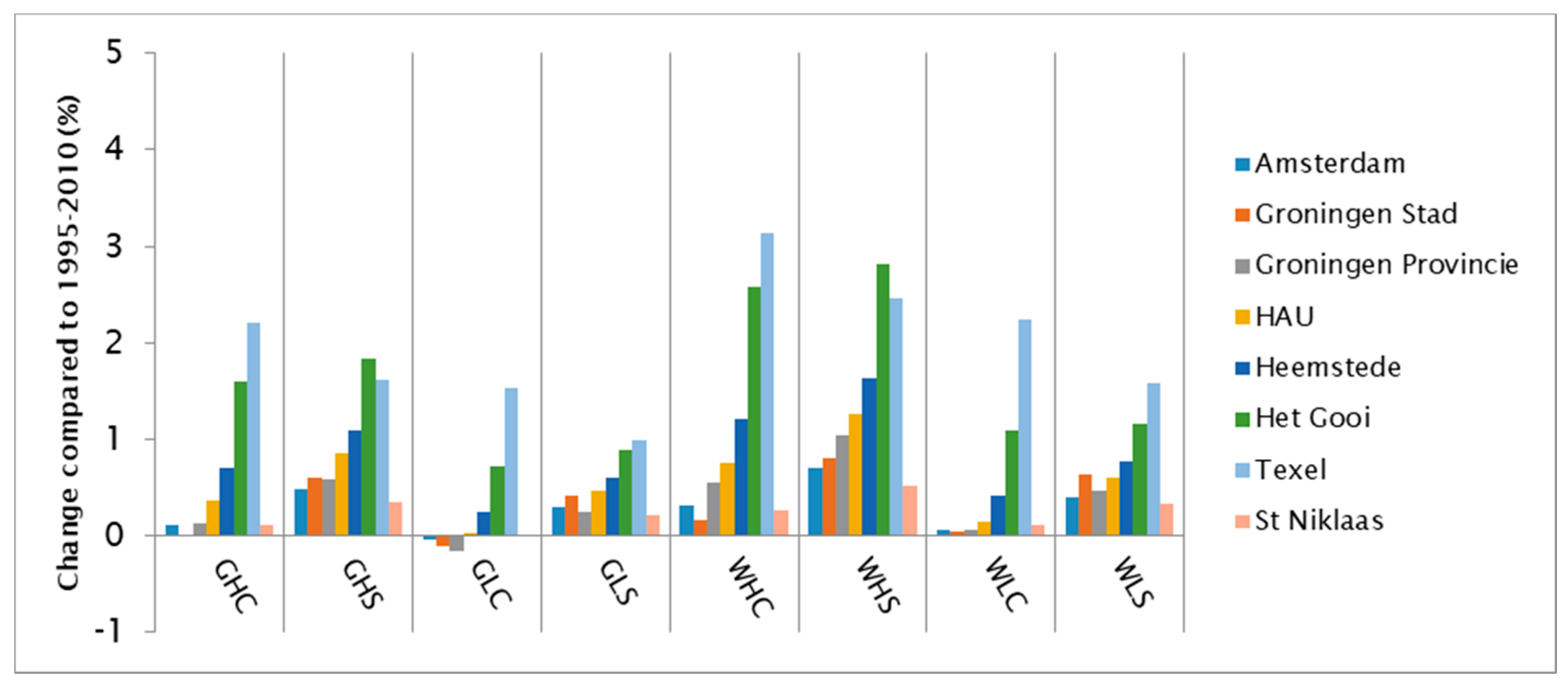
2.1.3. Scenario Development
- The degree of change in air circulation patterns above the Netherlands and Flanders (small or large);
- The rise in global temperature (+1 °C or +2 °C compared to the 1990 baseline);
- The change in vacation absence patterns (more concentrated or more spread out throughout the year).
2.2. Datasets
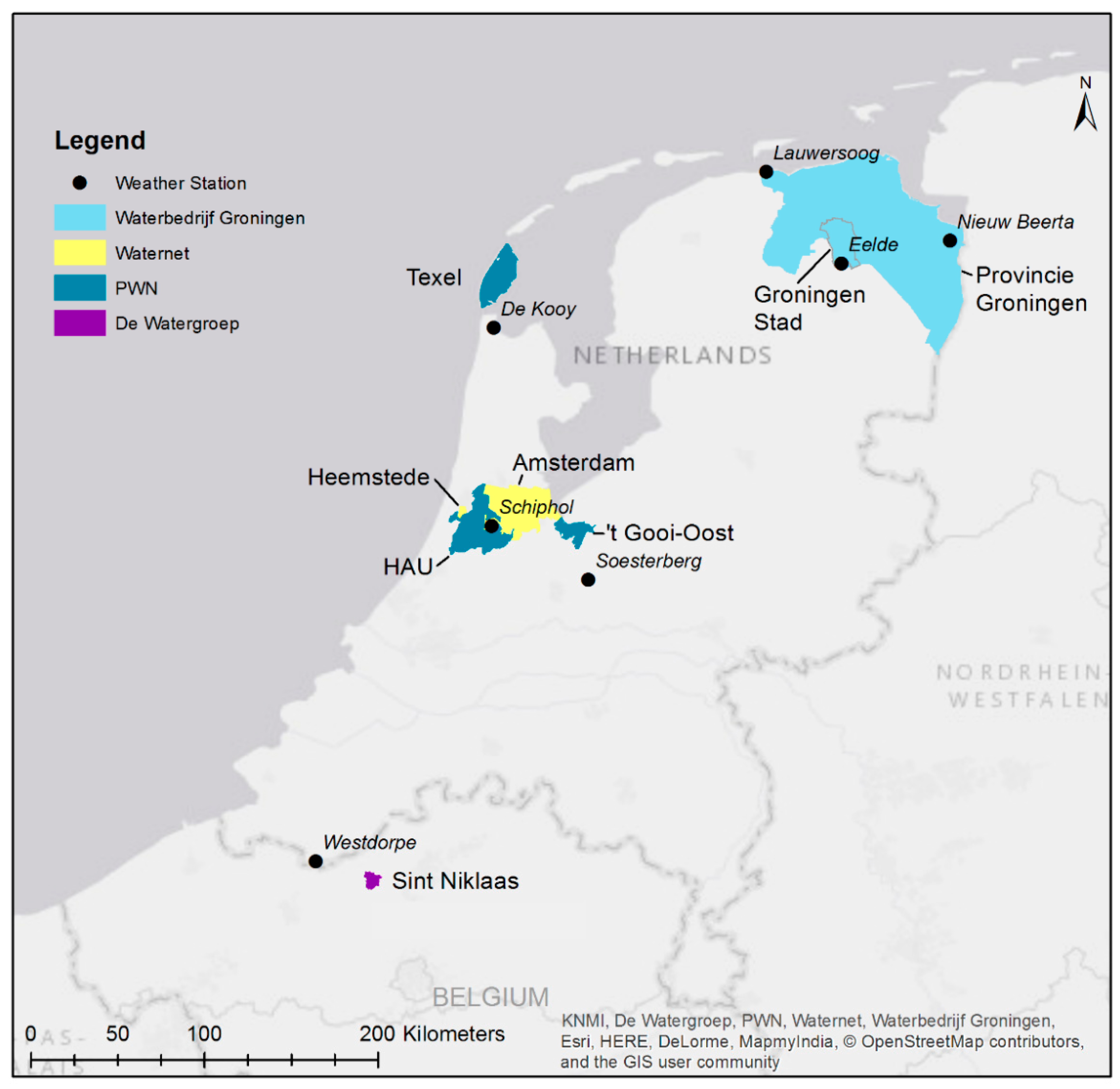
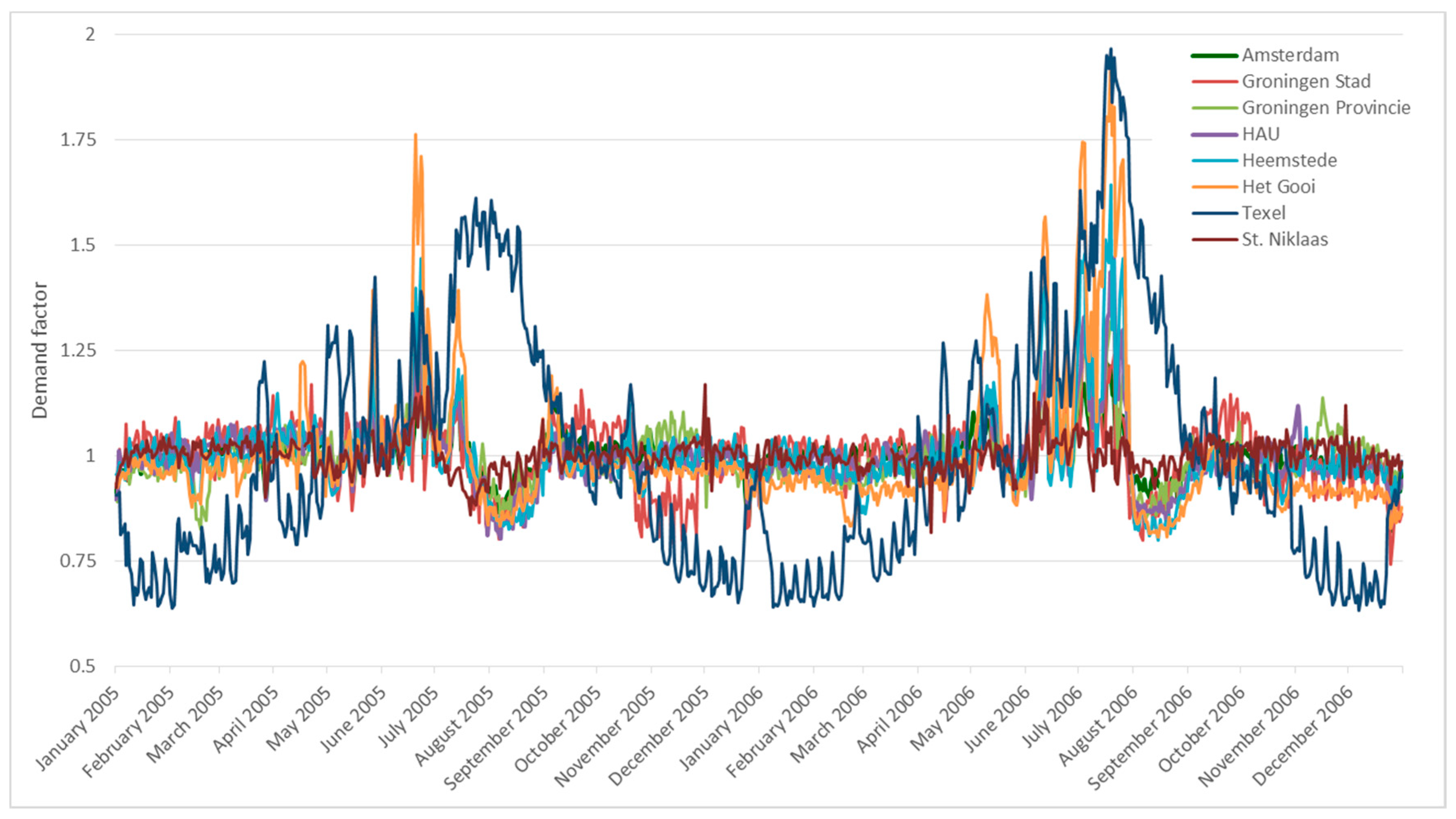
2.2.1. Water Supply Records
2.2.2. Meteorological Records
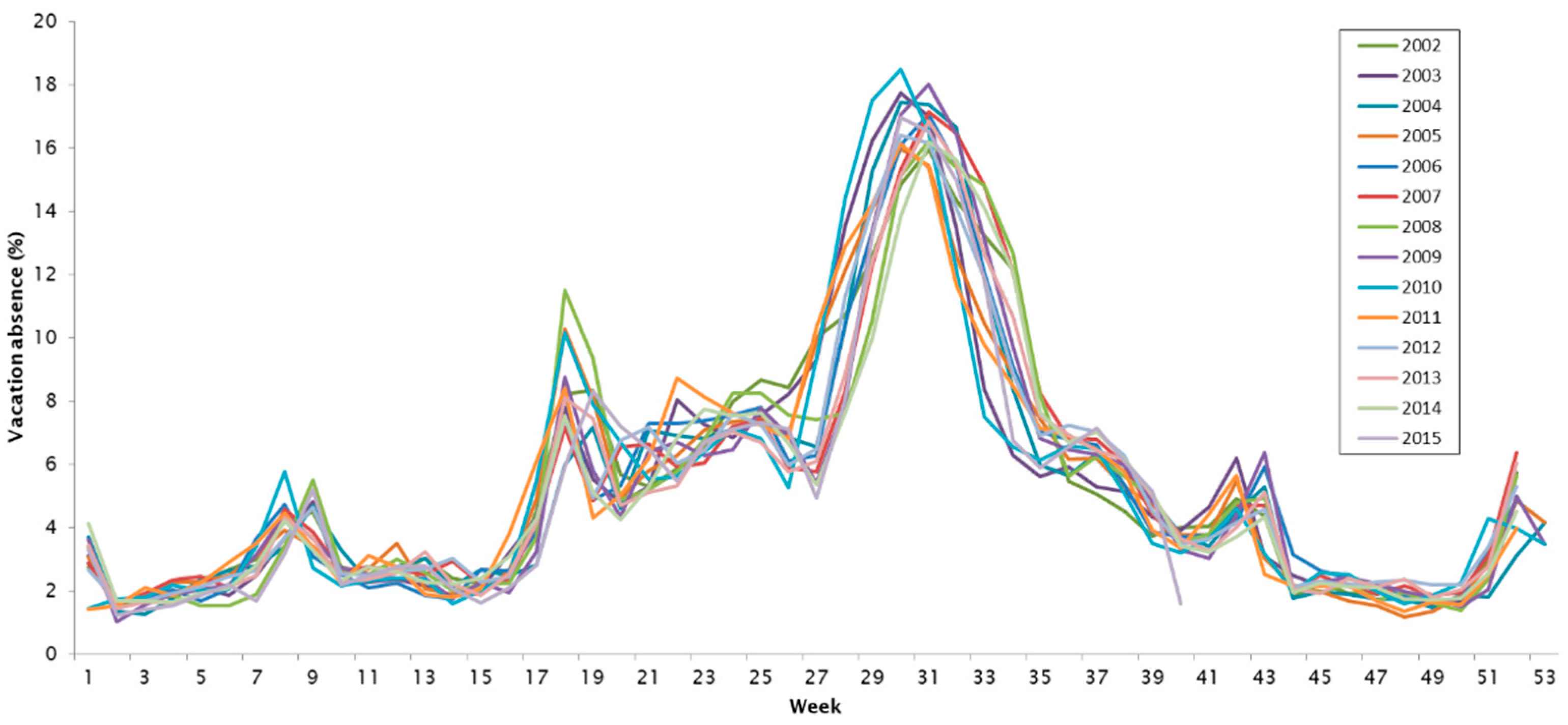
2.2.3. Vacation Absence Records
2.2.4. Other Data
3. Results and Discussion
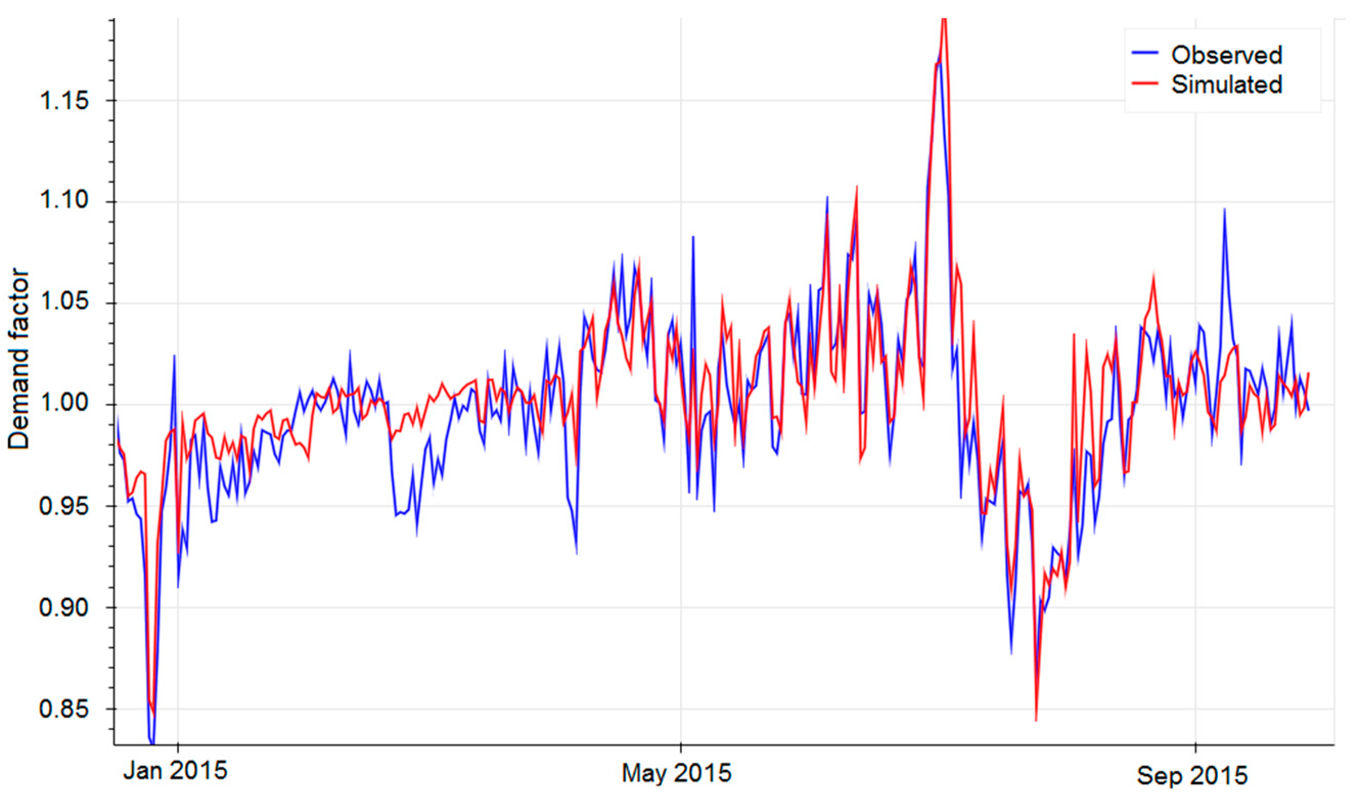
3.1. Regression Model
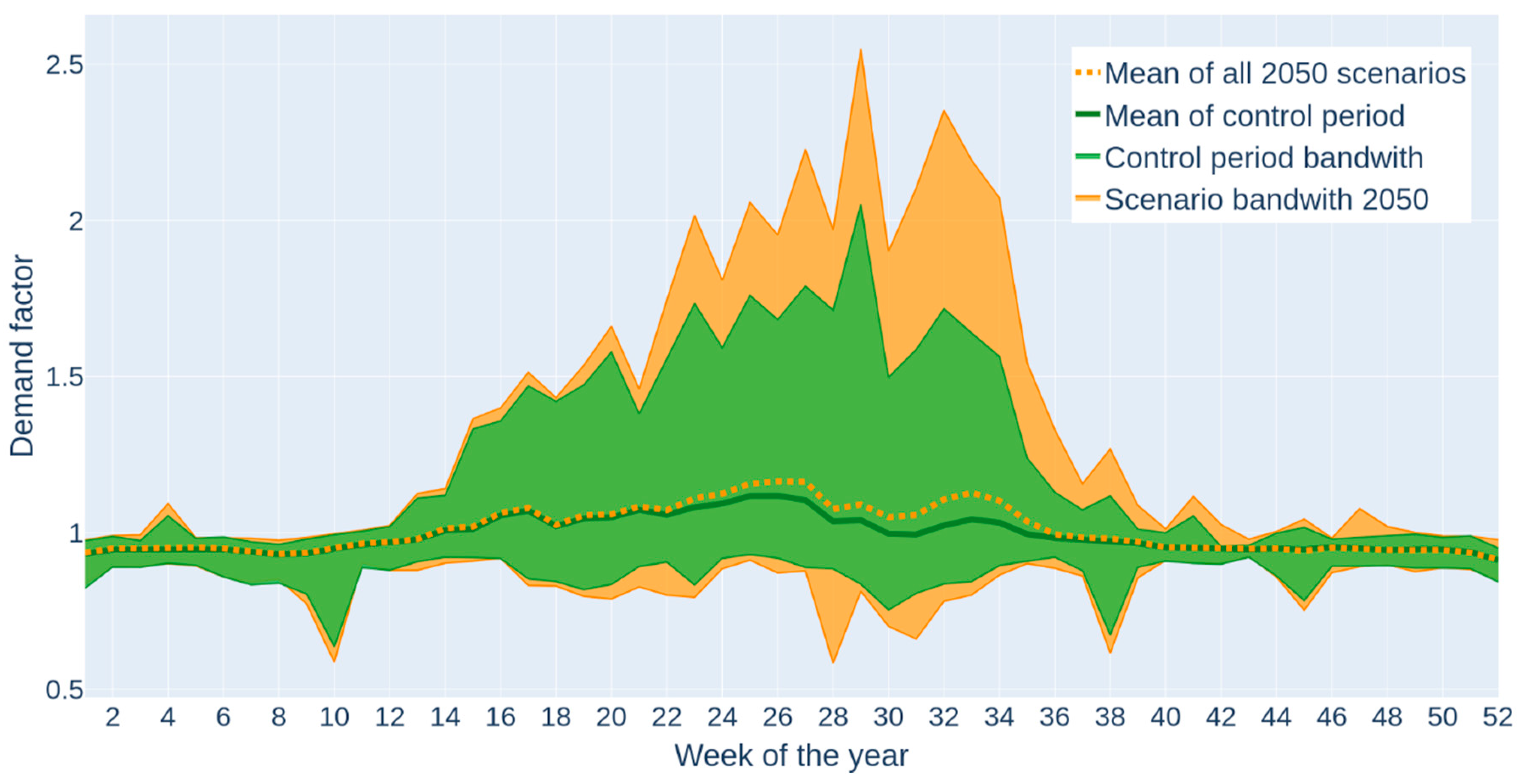
3.2. Average Water Demand
3.3. Peaking Factor
4. Conclusions
Author Contributions
Funding
Acknowledgments
Conflicts of Interest
References
- Zhang, X.; Buchberger, S.G.; van Zyl, J.E. A theoretical explanation for peaking factors. In Impacts of Global Climate Change, Proceedings of the World Water and Environmental Resources Congress 2005, Anchorage, AK, USA, 15–19 May 2005; American Society of Civil Engineers: Reston, VA, USA, 2005; pp. 1–12. [Google Scholar]
- Billings, R.B.; Jones, C.V. Forecasting Urban Water Demand; American Water Works Association: Denver, CO, USA, 2011. [Google Scholar]
- Murdock, S.H.; Albrecht, D.E.; Hamm, R.R.; Backman, K. Role of sociodemographic characteristics in projections of water use. J. Water Resour. Plan. Manag. 1991, 117, 235–251. [Google Scholar] [CrossRef]
- Wang, X.J.; Zhang, J.Y.; Shahid, S.; Guan, E.H.; Wu, Y.X.; Gao, J.; He, R.M. Adaptation to climate change impacts on water demand. Mitig. Adapt. Strateg. Glob. Chang. 2016, 21, 81–99. [Google Scholar] [CrossRef]
- Balling, R.C.; Gober, P.; Jones, N. Sensitivity of residential water consumption to variations in climate: An intraurban analysis of Phoenix, Arizona. Water Resour. Res. 2008, 44. [Google Scholar] [CrossRef] [Green Version]
- Donkor, E.A.; Mazzuchi, T.A.; Soyer, R.; Alan Roberson, J. Urban Water Demand Forecasting: Review of Methods and Models. J. Water Resour. Plan. Manag. 2014, 140, 146–159. [Google Scholar] [CrossRef]
- Alvisi, S.; Franchini, M.; Marinelli, A. A short-term, pattern-based model for water-demand forecasting. J. Hydroinform. 2007, 9, 39–50. [Google Scholar] [CrossRef] [Green Version]
- Bakker, M.; Van Duist, H.; Van Schagen, K.; Vreeburg, J.; Rietveld, L. Improving the Performance of Water Demand Forecasting Models by Using Weather Input. Procedia Eng. 2014, 70, 93–102. [Google Scholar] [CrossRef] [Green Version]
- Gardiner, V.; Herrington, P. Water Demand Forecasting; CRC Press: Boca Raton, FL, USA, 2014. [Google Scholar]
- Herrera, M.; Torgo, L.; Izquierdo, J.; Pérez-García, R. Predictive models for forecasting hourly urban water demand. J. Hydrol. 2010, 387, 141–150. [Google Scholar] [CrossRef]
- Zhou, S.L.; McMahon, T.A.; Walton, A.; Lewis, J. Forecasting daily urban water demand: A case study of Melbourne. J. Hydrol. 2000, 236, 153–164. [Google Scholar] [CrossRef]
- Cohen, S.J. Projected Increases in Municipal Water Use in the Great Lakes Due to CO2 induced Climatic Change. JAWRA J. Am. Water Resour. Assoc. 1987, 23, 91–101. [Google Scholar] [CrossRef]
- Goodchild, C.W. Modelling the Impact of Climate Change on Water Resources. Water Environ. J. 2003, 17, 8–12. [Google Scholar] [CrossRef]
- Babel, M.S.; Maporn, N.; Shinde, V.R. Incorporating future climatic and socioeconomic variables in water demand forecasting: A case study in Bangkok. Water Resour. Manag. 2014, 28, 2049–2062. [Google Scholar] [CrossRef]
- Toth, E.; Bragalli, C.; Neri, M. Assessing the significance of tourism and climate on residential water demand: Panel-data analysis and non-linear modelling of monthly water consumptions. Environ. Model. Softw. 2018, 103, 52–61. [Google Scholar] [CrossRef]
- Gössling, S.; Peeters, P.; Hall, C.M.; Ceron, J.P.; Dubois, G.; Scott, D. Tourism and water use: Supply, demand, and security. An international Review. Tour. Manag. 2012, 33, 1–15. [Google Scholar]
- Almutaz, I.; Ajbar, A.; Khalid, Y.; Ali, E. A probabilistic forecast of water demand for a tourist and desalination dependent city: Case of Mecca, Saudi Arabia. Desalination 2012, 294, 53–59. [Google Scholar] [CrossRef]
- Adamowski, J.; Fung Chan, H.; Prasher, S.O.; Ozga-Zielinski, B.; Sliusarieva, A. Comparison of multiple linear and nonlinear regression, autoregressive integrated moving average, artificial neural network, and wavelet artificial neural network methods for urban water demand forecasting in Montreal, Canada. Water Resour. Res. 2012, 48. [Google Scholar] [CrossRef]
- Ghiassi, M.; Zimbra, D.K.; Saidane, H. Urban water demand forecasting with a dynamic artificial neural network model. J. Water Resour. Plan. Manag. 2008, 134, 138–146. [Google Scholar] [CrossRef]
- Sadiq, W.A.; Karney, B.W. Modeling water demand considering impact of climate change—A Toronto case study. Eff. Model. Urban Water Syst. Monogr. 2005, 13. [Google Scholar] [CrossRef]
- Vapnik, V. The Nature of Statistical Learning Theory; Springer Science & Business Media: Berlin/Heidelberg, Germany, 2013. [Google Scholar]
- Auria, L.; Moro, R.A. Support Vector Machines (SVM) as a Technique for Solvency Analysis; Discussion Papers of DIW Berlin 811; DIW Berlin: Berlin, Germany, 2008. [Google Scholar]
- Smets, K.; Verdonk, B.; Jordaan, E.M. Evaluation of performance measures for SVR hyperparameter selection. In Proceedings of the 2007 International Joint Conference on Neural Networks, Orlando, FL, USA, 12–17 August 2007; IEEE: Piscataway, NJ, USA, 2007. [Google Scholar]
- Scholkopf, B.; Smola, A.J. Learning with Kernels: Support Vector Machines, Regularization, Optimization, and Beyond; MIT Press: Cambridge, MA, USA, 2001. [Google Scholar]
- Pedregosa, F.; Varoquaux, G.; Gramfort, A.; Michel, V.; Thirion, B.; Grisel, O.; Blondel, M.; Prettenhofer, P.; Weiss, R.; Dubourg, V.; et al. Scikit-learn: Machine learning in Python. J. Mach. Learn. Res. 2011, 12, 2825–2830. [Google Scholar]
- Faranda, D.; Lucarini, V.; Turchetti, G.; Vaienti, S. Numerical convergence of the block-maxima approach to the generalized extreme value distribution. J. Stat. Phys. 2011, 145, 1156–1180. [Google Scholar] [CrossRef]
- Ferreira, A.; de Haan, L. On the block maxima method in extreme value theory: PWM estimators. Ann. Stat. 2015, 43, 276–298. [Google Scholar] [CrossRef] [Green Version]
- Lang, M.; Ouarda, T.; Bobée, B. Towards operational guidelines for over-threshold modeling. J. Hydrol. 1999, 225, 103–117. [Google Scholar] [CrossRef]
- Kyselý, J.; Picek, J.; Beranová, R. Estimating extremes in climate change simulations using the peaks-over-threshold method with a non-stationary threshold. Glob. Planet. Chang. 2010, 72, 55–68. [Google Scholar] [CrossRef]
- Méndez, F.J.; Menéndez, M.; Luceño, A.; Losada, I.J. Estimation of the long-term variability of extreme significant wave height using a time-dependent peak over threshold (pot) model. J. Geophys. Res. Ocean. 2006, 111. [Google Scholar] [CrossRef]
- Renard, B.; Lang, M.; Bois, P. Statistical analysis of extreme events in a non-stationary context via a Bayesian framework: Case study with peak-over-threshold data. Stoch. Environ. Res. Risk Assess. 2006, 21, 97–112. [Google Scholar] [CrossRef]
- Martins, E.S.; Stedinger, J.R. Generalized maximum-likelihood generalized extreme-value quantile estimators for hydrologic data. Water Resour. Res. 2000, 36, 737–744. [Google Scholar] [CrossRef]
- Gilleland, E.; Katz, R.W. extRemes 2.0: An extreme value analysis package in R. J. Stat. Softw. 2016, 72, 1–39. [Google Scholar]
- Bakker, A. Time Series Transformation Tool Version 3.1—Description of the Program to Generate Time Series Consistent with the KNMI’14 Climate Scenarios; KNMI: De Bilt, The Netherlands, 2015. [Google Scholar]
- Van Den Hurk, B.; Siegmund, P.; Tank, A.K. KNMI’14: Climate Change Scenarios for the 21st Century—A Netherlands Perspective; KNMI: De Bilt, The Netherlands, 2014. [Google Scholar]
- Van Dijk Hans, J.; QJC, V.J.; De Moel Peter, J. Drinking Water: Principles and Practices; World Scientific: Singapore, 2006. [Google Scholar]
- Rijtema, P. Calculation Methods of Potential Evapotranspiration; ICW: Glasgow, UK, 1959. [Google Scholar]
- CBS. Continu Vakantie Onderzoek (CVO). 2019. Available online: https://www.cbs.nl/nl-nl/onze-diensten/methoden/onderzoeksomschrijvingen/korte-onderzoeksbeschrijvingen/continu-vakantie-onderzoek--cvo---tot-2017 (accessed on 20 May 2019).


| Supply Area | Number of Inhabitants (×1000) | Type | Average Demand (×1000 m3/d) | Average Demand Per Capita (m3/d) | Water Utility |
|---|---|---|---|---|---|
| Amsterdam | 955 | Urban | 191 | 0.20 | Waternet |
| Groningen Provincie | 394 | Suburban/rural | 91 | 0.23 | Waterbedrijf Groningen |
| Groningen Stad | 198 | Urban | 33 | 0.17 | Waterbedrijf Groningen |
| HAU | 215 | Suburban | 39 | 0.18 | PWN |
| Heemstede | 26 | Urban | 4 | 0.15 | Waternet |
| Het Gooi | 112 | Rural | 20 | 0.18 | PWN |
| Texel | 14 | Rural | 4 | 0.29 | PWN |
| Sint Niklaas | 51 | Urban | 7 | 0.14 | De Watergroep |
| Variable | Unit | Description |
|---|---|---|
| P | mm | Precipitation |
| E | mm | Reference evaporation according to Makkink [37] |
| Tav | °C | Average daily temperature |
| Tmax | °C | Maximum daily temperature |
| Q | J/cm2 | Solar irradiance |
| Supply Area | C | R2 Training | R2 Test | |
|---|---|---|---|---|
| Amsterdam | 0.022 | 0.018 | 0.70 | 0.63 |
| Groningen Provincie | 0.05 | 0.022 | 0.72 | 0.66 |
| Groningen Stad | 0.12 | 0.04 | 0.60 | 0.50 |
| HAU | 0.025 | 0.034 | 0.62 | 0.60 |
| Heemstede | 0.04 | 0.027 | 0.60 | 0.61 |
| Het Gooi | 0.10 | 0.020 | 0.80 | 0.77 |
| Texel | 0.14 | 0.038 | 0.93 | 0.91 |
| Sint Niklaas | 0.019 | 0.013 | 0.44 | 0.39 |
| Supply Area | Peaking Factor Current | Peaking Factor 2050 (Min–Max) | Relative Change (%, Min–Max) |
|---|---|---|---|
| Amsterdam | 1.19 | 1.21–1.28 | 1.7–7.6 |
| Groningen Provincie | 1.30 | 1.30–1.38 | 0–6.2 |
| Groningen Stad | 1.21 | 1.24–1.36 | 2.5–12 |
| HAU | 1.34 | 1.40–1.54 | 4.5–15 |
| Heemstede | 1.50 | 1.58–1.75 | 5.3–16.7 |
| Het Gooi | 1.90 | 1.99–2.31 | 4.7–21.6 |
| Texel | 1.99 | 1.93–2.24 | −3–12.6 |
| Sint Niklaas | 1.15 | 1.17–1.24 | 1.7–7.8 |
© 2019 by the authors. Licensee MDPI, Basel, Switzerland. This article is an open access article distributed under the terms and conditions of the Creative Commons Attribution (CC BY) license (http://creativecommons.org/licenses/by/4.0/).
Share and Cite
Vonk, E.; Cirkel, D.G.; Blokker, M. Estimating Peak Daily Water Demand under Different Climate Change and Vacation Scenarios. Water 2019, 11, 1874. https://doi.org/10.3390/w11091874
Vonk E, Cirkel DG, Blokker M. Estimating Peak Daily Water Demand under Different Climate Change and Vacation Scenarios. Water. 2019; 11(9):1874. https://doi.org/10.3390/w11091874
Chicago/Turabian StyleVonk, Erwin, Dirk Gijsbert Cirkel, and Mirjam Blokker. 2019. "Estimating Peak Daily Water Demand under Different Climate Change and Vacation Scenarios" Water 11, no. 9: 1874. https://doi.org/10.3390/w11091874
APA StyleVonk, E., Cirkel, D. G., & Blokker, M. (2019). Estimating Peak Daily Water Demand under Different Climate Change and Vacation Scenarios. Water, 11(9), 1874. https://doi.org/10.3390/w11091874