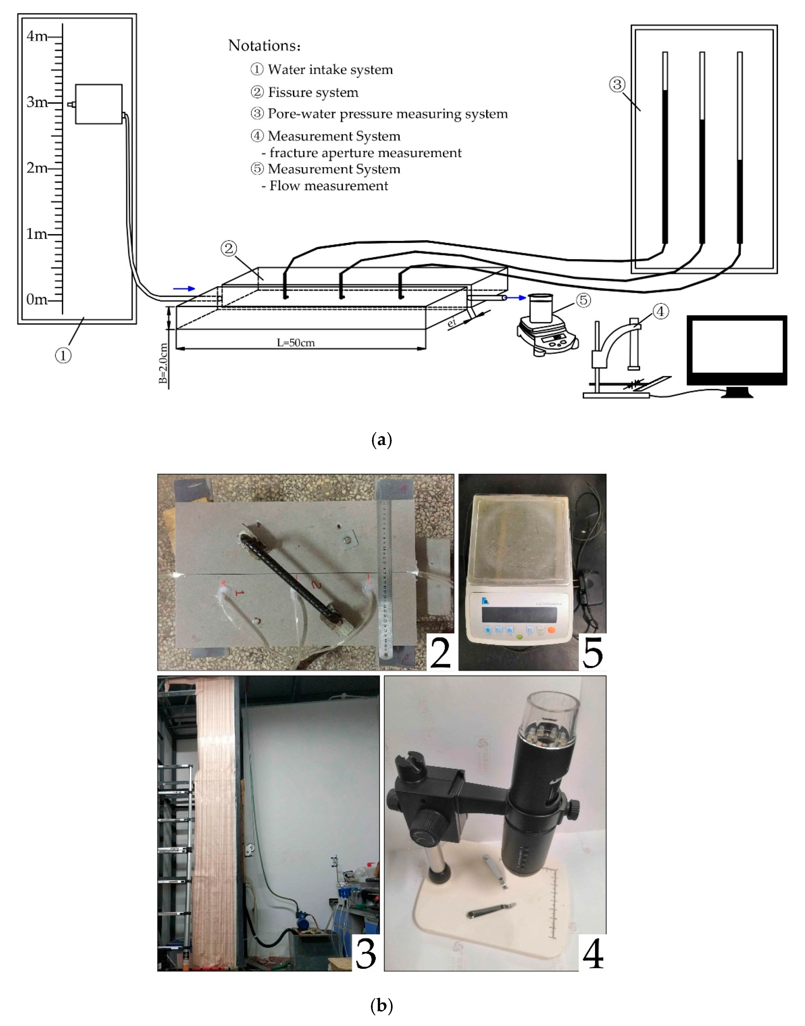
3.1. Data Analysis of Laboratory Physical Model Test
In the physical experiment of single fracture, aperture e (0.77, 1.18, 1.97, 2.73 mm) was used as the test variable. The pressure gradient
corresponding to different flow Q under different fracture apertures was obtained and is analyzed in
Table 2 and plotted in
Figure 3.
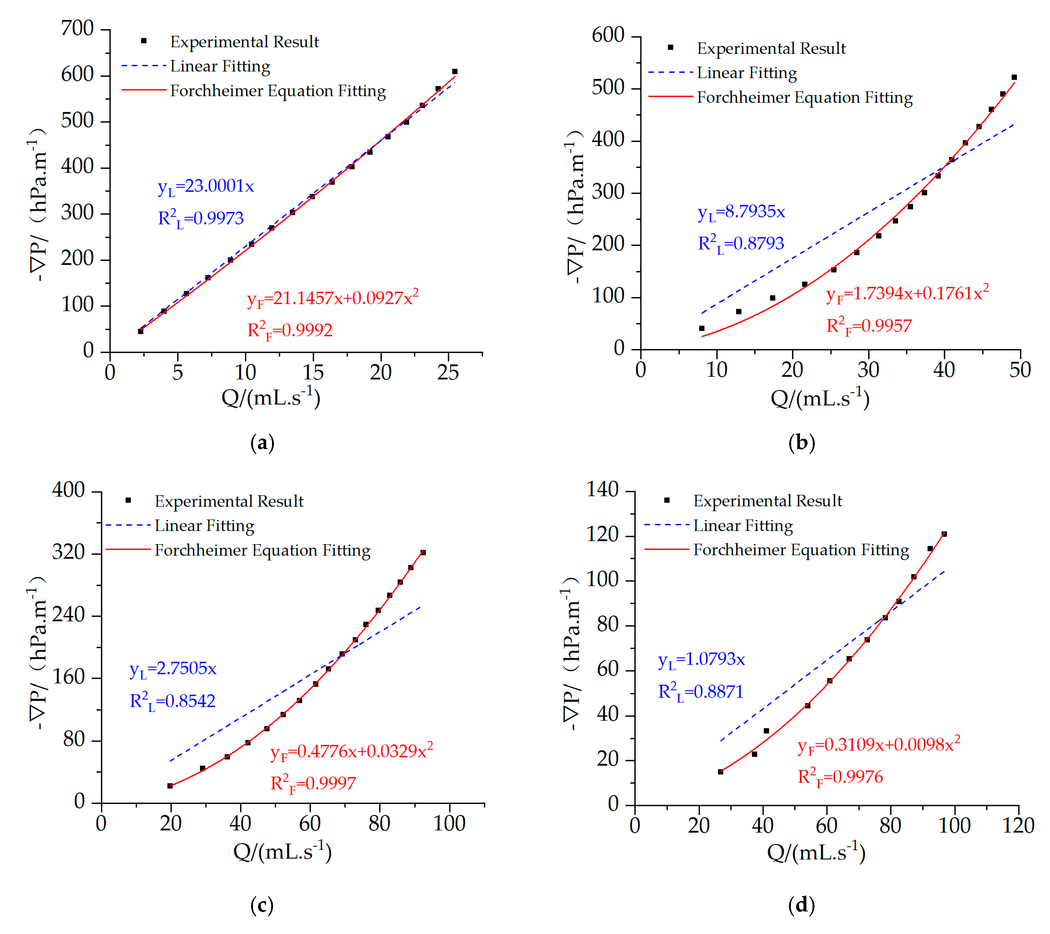
All of the scatterplots of the volume of flow and the pressure gradient are similar to a parabola except at e = 0.77 mm, which is in accordance with the results that reported by Shu et al. [
22], Wang et al. [
35], and Akinbodewa et al. [
36]. They show obvious non-Darcian flow in the test, since the shape of the line is not linear but parabolic. The transition from linear to nonlinear behavior is like that described by Andrade et al. [
37].
The linear equation does not perform well when used to fit the relationship between the volume of flow and the pressure gradient except at e = 0.77 mm (Absolute Average Relative Error, AAREL = 4.6–31.5%), while the Forchheimer equation fits well with larger determination coefficients (AAREF = 1.1–9.1%). The sum of squares of residual errors of the Forchheimer equation was one to three orders of magnitude smaller than that of the linear Equation and has smaller values of Akaike information criterion (AIC) and Schwarz’s criterion (SC). Thus, the Forchheimer equation is more suitable for describing the law of flow movement in fissures.
3.2. Comparison between Experiment and Simulation
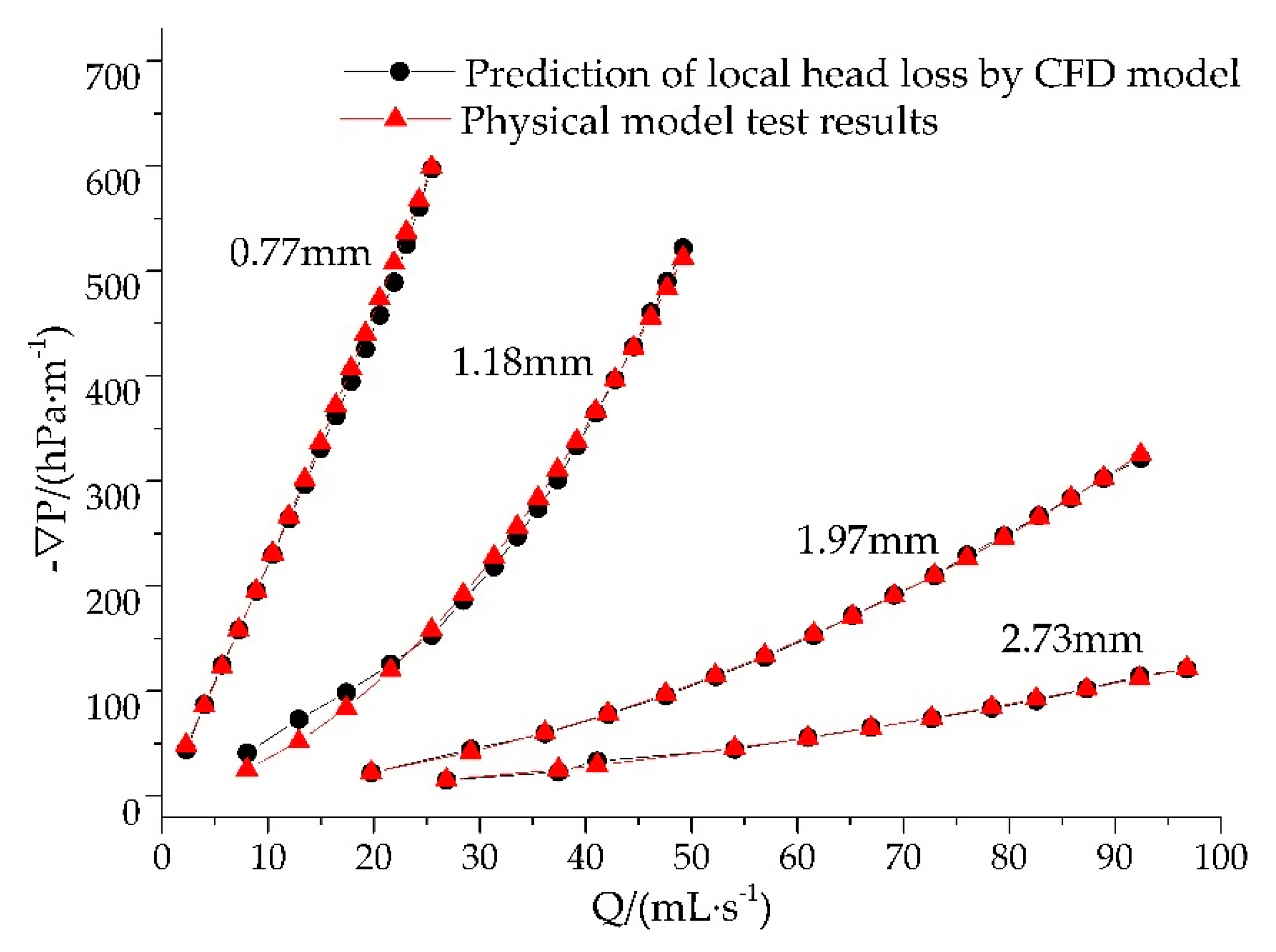
The realizable k–ε model was used to calculate the pressure drop in a single fracture with different apertures. The results of the CFD model were compared with those of the laboratory test at the same fracture aperture.
Figure 4 shows that all results of the CFD model were close to those of the physical test, with the determination coefficient
R2 ranging from 0.9643 to 0.9951. As is well-known, when the determination coefficient
R2 of a non-intercepting fitting curve is close to one, the two sets of data are similar.
To validate the above conclusion, Pearson’s correlation coefficient was employed for further analysis. As shown in
Table 3, all Pearson’s correlation coefficients were close to one, indicating a strong correlation between the CDF modeling results and the numerical results, which is consistent with
Figure 4. This means that the CFD model accurately simulated the flow of fracture fluid under specified conditions, consistent with the results of Wang et al. [
38].
From the above analysis, it can be inferred that the CFD model was useful for studying the characteristics of flow in fractures, and it has potential in flexural crack modelling.
3.3. Effect of Fracture Shape on Head Loss
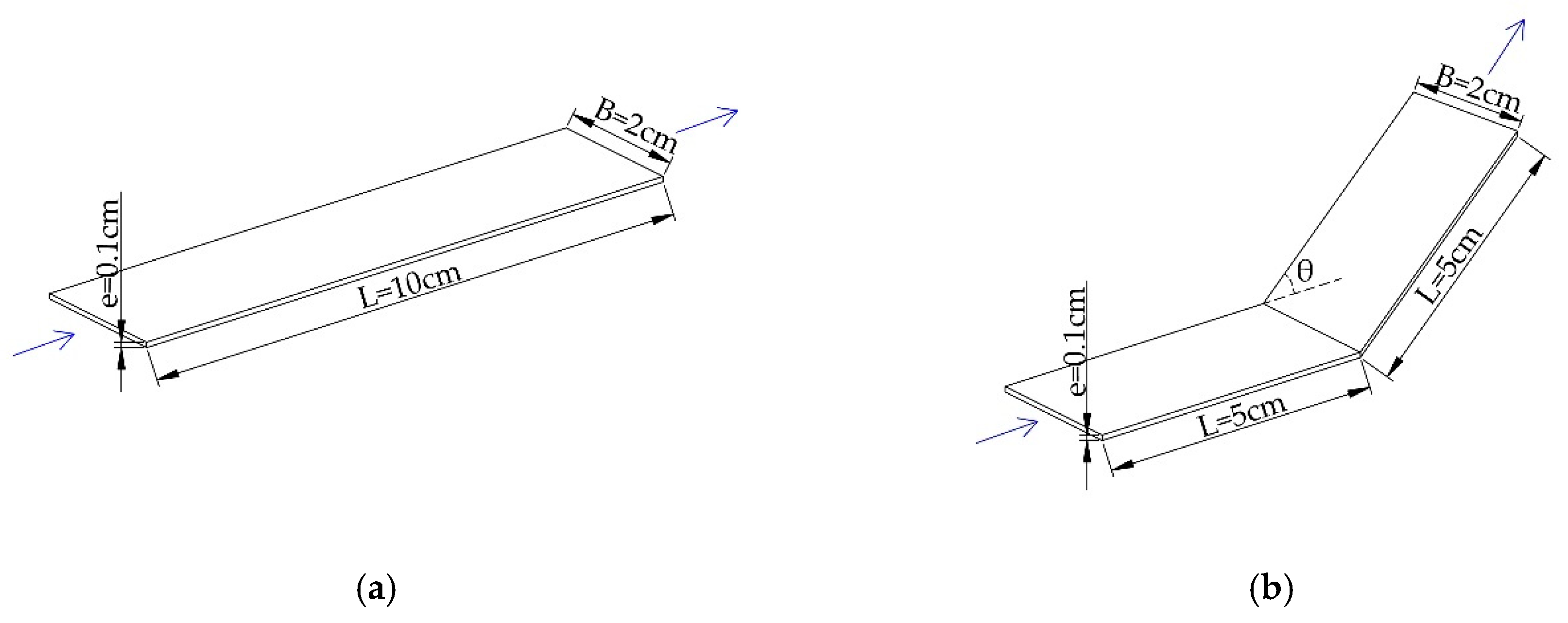
It is known that the local head loss changes when the fracture aperture changes. In order to study the relationship between the fracture shape (corner θ) and the local head loss, the fracture width is should be fixed first.
Bernoulli’s equation represents the conservation of mechanical energy of an ideal fluid and can represent the process of constant energy change of the fluid per unit mass, the relation of element flow on any section, as shown in Equation (5) [
39]:
Based on this, the energy equation of the real fluid with energy loss at the cross-section of upstream and downstream can be written as follows [
28]:
where
v is flow velocity in the fracture, (m·s
−1);
g is gravitational acceleration, 9.8 m/s
2;
is the local head loss caused by the shape of the fissure (θ);
is frictional head loss; “1” and “2” are cross-sectional symbols of upstream and downstream, respectively, and α is the total flow correction factor. For fully developed turbulent flow, α ≈ 1.
The total head loss from upstream to downstream is set to
, which can be written as:
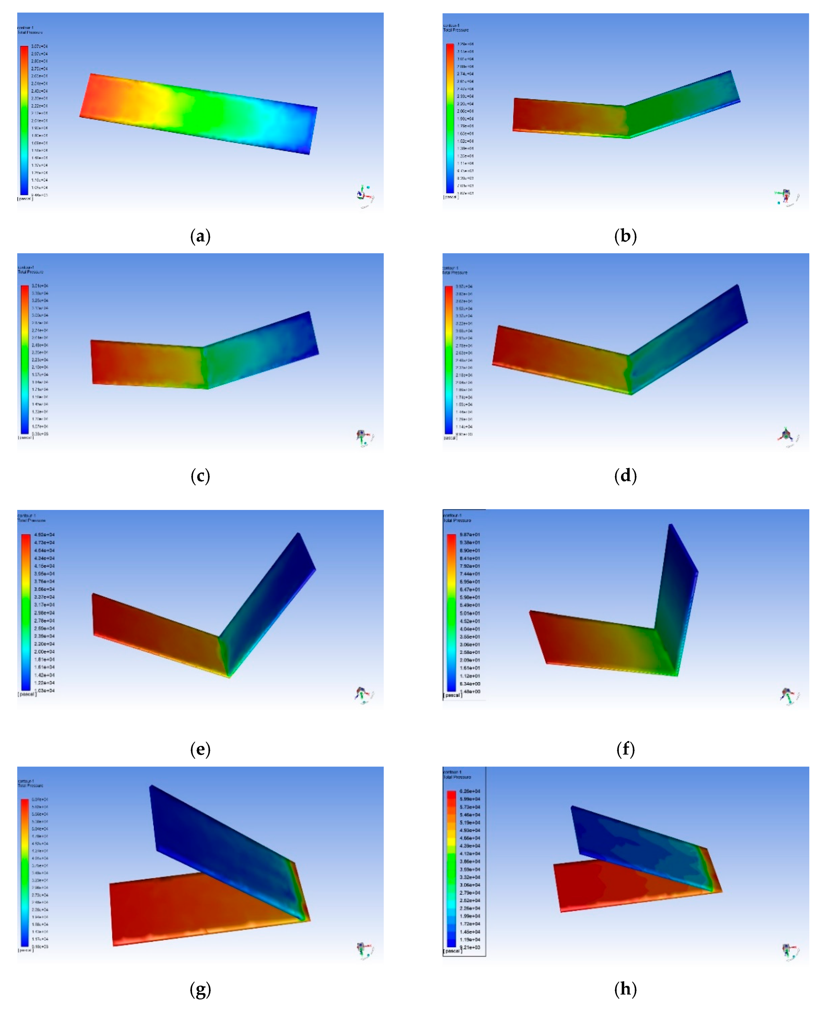
To study the local head loss caused by the shape of the fracture, a comparative numerical model was constructed with a fracture aperture of 1 mm, length of 100 mm, width of 20 mm, and the value of θ at zero. Under the same conditions, we established seven numerical models with θ = 30, 45, 60, 90, 120, 135, and 150 degrees. The contour maps of pressure at flexural crack with different θ can be seen in
Figure 5.
In the CFD numerical model test, except for the shape of the fracture (θ), the boundary conditions and parameters of each model were the same, because of which the frictional head loss of each model was the same (
). When θ = 0, the local head loss caused by fracture shape was 0 (
). By comparing the results of these models, the local head loss caused at different values of θ at different flow velocities was calculated.
where Δ
H0 is the head loss when θ = 0, and Δ
Hi is that when θ = i.
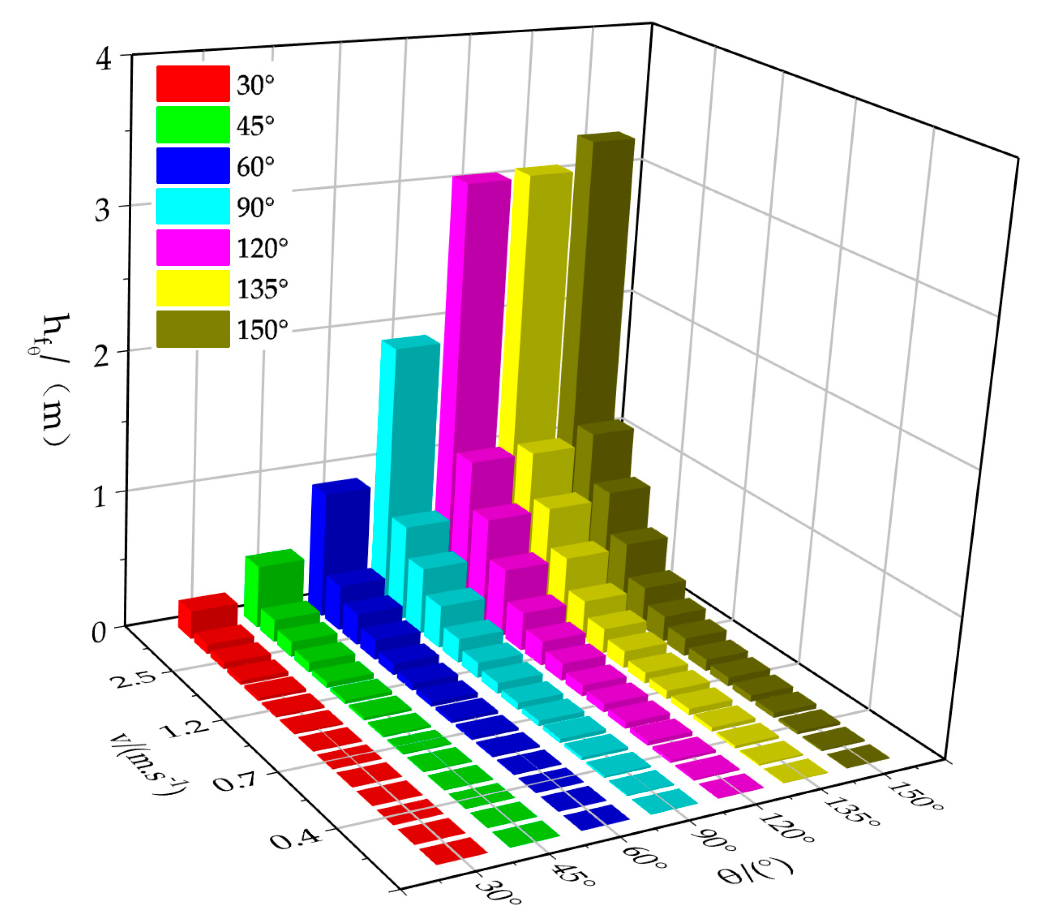
The local head loss of each flexural crack at different angles (θ) is shown in
Figure 6. It is clear that local head loss caused by fracture shape increased with the flow velocity and the crossed angle.
The velocity distribution in the water-crossing section is more uneven in non-Darcian flow, and there is shear stress between the layers of flow [
40]. When the fluid flowed through the turning point of the flexural crack in a state of turbulence where the inertial force played a dominant role, the flow could not change direction abruptly along the fracture shape, with the consequence that the mainstream of fluids was separated from the side-wall of the fracture, and vortices were generated [
41]. The eddy current and mainstream were superimposed, and spiral motion occurred downstream of the corner. In this motion, the generation, collision, merging, splitting, and disappearance of the eddy current consumed a large amount of the fluid’s mechanical energy, which was the local head loss caused by the shape of the fracture.
It has been found that the larger θ is, the more active the motion of the eddy current is, and the greater the head loss is [
42]. This is consistent with the results of this study. Some researchers have observed that initial pressure on the fluid controls its instantaneous flow rate in pipes. When the shape of the pipe remains constant, the local resistance loss increases with the Reynolds number [
43], which agrees with the results of this study. Therefore, flow velocity and fracture shape are the important factors affecting local head loss.
3.4. Establishment of Fast Calculation of Local Head Loss
A pairwise correlation analysis between the independent variables (θ and
v) and the dependent variable (local head loss
hf) was quantitatively represented using the Pearson coefficient, as shown in
Table 4.
From the above tables, it is clear that Pearson’s correlation coefficient had the value P
v > P
θ, indicating that the influence of
v on local head loss was greater than that of θ. As the flow velocity and fracture shape are positively correlated with head loss, the calculation model,
should consider all of them, and can be expressed as [
43]:
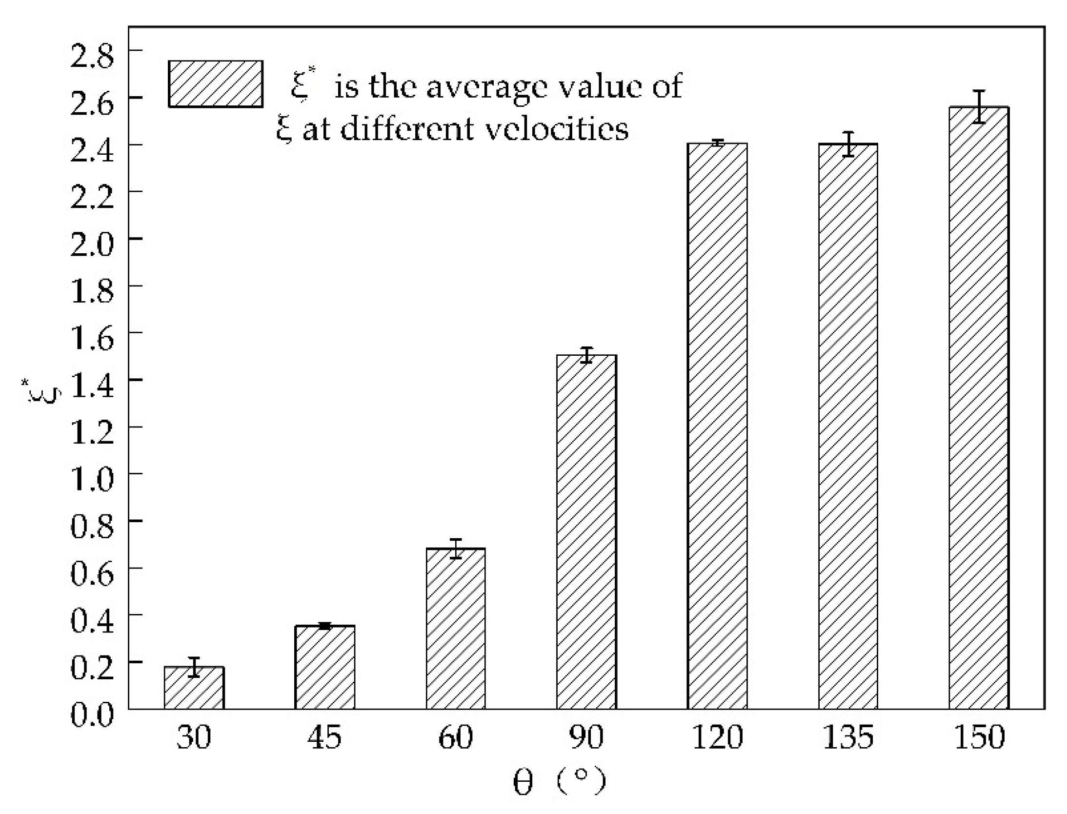
is the coefficient of local head loss that is usually related to the geometry of the member and the nature of the fluid flowing through the member, and it can be rewritten as:
is the average value of
at different velocities. As shown in
Figure 7, the value of
is nonlinearly positively correlated with θ, and error caused by changes in the flow velocity is minimal. Therefore, the calculation model for the local head loss coefficient is a function related only to the shape of the fracture but not to velocity.
The curve characteristic observed is S-shaped, which is somewhat similar to a logistic function. The logistic function was first used to reflect a nutritional relationship to population mathematical model in 1838, but it has been found useful in many fields. The original logistic function is:
where t is the time variable, and a, b, and C are the model constants.
The deformation of logistic equation [
44] was used to fit the head loss coefficient as follows:
The crossed angle (θ) was the independent variable with a range of 0–180 degrees. , , , and p are the characteristic parameters of the equation. For our study, they were = 0.1673, = 3.7346, = 88.0791, and p = 3.7179.
Based on the Equation (12), we can quickly calculate the local head loss:
where
g is the gravity coefficient, with the value of 9.8 m/s
2.
3.5. The Use of Fast Calculation Equation of Head Loss
During fluid flow, the head loss includes the sum of the frictional head loss and the local head loss listed in Equation (7), while in
Section 3.1, we found that “∇P-Q” can be well characterized by the Forchheimer equation. Therefore, the frictional head loss can be calculated according to the Forchheimer equation obtained previously. From numeric simulation, the fitting Forchheimer equation between hydraulic gradient (
J) and flow velocity with fracture aperture of 1 mm and transverse width of 2 cm was obtained, with
R2 > 0.99, as follows:
Considering the distance of frictional head loss, the calculation equation of frictional head loss can be obtained as:
where
L is the length of the fracture.
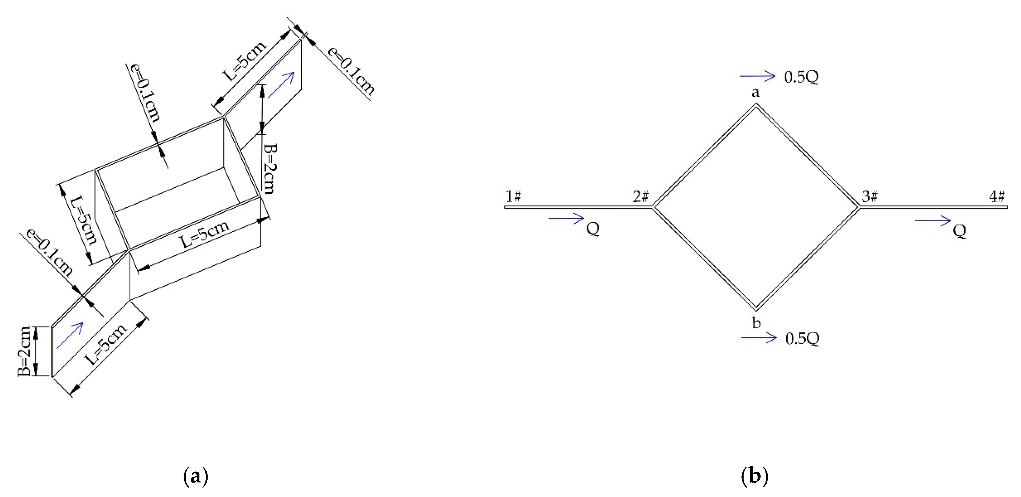
The above quantitative equations (Equations (13) and (15)) can be applied to the calculation of head loss when the crack with aperture is 1 mm and transverse width is 2 cm. To apply this, a network fissure with four nodes 1#–4# was set as shown in
Figure 8.
According to Kirchhoff’s law, the flow equation at the node was established:
Assuming that the flow velocity at the entrance (1#) and exit (4#) is
v, the flow velocity in each flow path is:
In
Figure 7, We can divide the network fracture into multiple single fractures and local loss occurrence points, so the head loss of the fracture network is the sum of them:
where:
Among the Equations (19) and (20),
hl(1-2),
hl(2-a),
hl(a-3),
hl(2-b),
hl(b-3), and
hl(3-4) refer to the frictional head loss of the fracture segment of (1-2), (2-a), (a-3), (2-b), (b-3), and (3-4);
hf(1-2-a),
hf(2-a-3),
hf(a-3-4),
hf(1-2-b),
hf(2-b-3), and
hf(b-3-4)refer to the local head loss at the positions where the direction of flow changes. Parameters of each fracture or intersection point are listed in
Table 5 and
Table 6.
The head losses calculated are listed in
Table 7.
From
Table 7, it can be seen that local head loss accounts for a small proportion when the flow velocity is small, but it grows fast as the flow velocity increases because local head loss is proportional to the square of speed. Water inrush from the underground projects, such as tunnels, is always very fast, so the local head loss is necessary to be taken into consideration when doing water inflow predication. In addition, parameters of Equations (13) and (15) need to be recalibrated before use because they are obtained from the specific conditions when the fracture aperture is 1 mm and its width is 20 mm.


