Article

Analytical Solutions for Unsteady Groundwater Flow in an Unconfined Aquifer under Complex Boundary Conditions

School of Earth Science and Engineering, Hohai University, Nanjing 210098, China
*
Author to whom correspondence should be addressed.
Water 2020, 12(1), 75; https://doi.org/10.3390/w12010075
Submission received: 23 October 2019 / Revised: 18 December 2019 / Accepted: 21 December 2019 / Published: 24 December 2019
(This article belongs to the Section Hydraulics and Hydrodynamics)

Abstract

:
The response laws of groundwater dynamics on the riverbank to river level variations are highly dependent on the river level fluctuation process. Analytical solutions are widely used to infer the groundwater flow behavior. In analytical calculations, the river level variation is usually generalized as instantaneous uplift or stepped, and then the analytical solution of the unsteady groundwater flow in the aquifer is derived. However, the river level generally presents a complex, non-linear, continuous change, which is different from the commonly used assumptions in groundwater theoretical calculations. In this article, we propose a piecewise-linear approximation to describe the river level fluctuation. Based on the conceptual model of the riverbank aquifer system, an analytical solution of unsteady groundwater flow in an unconfined aquifer under complex boundary conditions is derived. Taking the Xiluodu Hydropower Station as an example, firstly, the monitoring data of the river level during the period of non-impoundment in the study area are used to predict the groundwater dynamics with piecewise-linear and piecewise-constant step approximations, respectively, and the long-term observation data are used to verify the calculation accuracy for the different mathematical models mentioned above. During the reservoir impoundment period, the piecewise-linear approximation is applied to represent the reservoir water level variation, and to predict the groundwater dynamics of the reservoir bank.

1. Introduction

The interaction between groundwater and surface water is a universal phenomenon in the natural world and an important part of the terrestrial hydrological cycle [1,2]. In the case of hydraulic connections between surface rivers and unconfined water, the river level variation is the key factor affecting the groundwater dynamics on both sides of the river [3,4,5]. When the river level rises, surface water infiltrates into the groundwater. This can lead to environmental and geological problems [2,4,6,7,8] such as solute transport, groundwater pollution, reservoir immersion, and land salinization. Therefore, understanding surface–subsurface water interactions and being able to compute the effect of these interactions are essential to address environmental and geological problems.
Analytical methods and numerical simulations are often used for studying the unsteady groundwater flow caused by river level variations. In general, the numerical simulation method requires complicated algorithms to solve the problem of convergence and conservation of mass for specific models [9,10,11] and to obtain an approximate solution. The analytical solution needs to obey strict assumptions [12]. However, it has intuitive and concise expression, and it is relatively easy to obtain unsteady groundwater flow laws and give an effective approach to evaluate the calculation accuracy. For simplified mathematical models, the commonly used analytical solutions are usually based on the condition that the river level remains constant after the instantaneous change has been completed. In addition, the J.G. Ferris model [13] is a classical method to solve such problems. However, the actual change of the river level is different from the assumptions in groundwater flow theoretical calculations, which are frequently affected by many factors, mainly depending on the topographic, geomorphological, hydrological, and meteorological conditions of the basin; the hydraulic characteristics of the basin itself; and the influence of artificial regulation. Meanwhile, the river level variation has its own characteristics: Firstly, the water level varies nonlinearly and continuously with time; secondly, the water level presents periodic variation; thirdly, the water level varies sharply in the wet season and gently in the dry season. For mathematical simplicity, the piecewise-constant step approximation is the most commonly used approach to represent the river level variation, and then such a problem is analyzed by the superposition principle combined with the solution of the classical model [14]. However, when the river level variation is more complex, the piecewise-constant step approach needs more segments to describe the variation process, and the calculation is more cumbersome. Moreover, the commonly used approach to represent the river level variation may not always be sufficient to capture important details in the observed hydraulic transient and continuous variation characteristics, which will also result in great errors to the unsteady groundwater flow calculation. For cases where the river level variability exhibits increasing or decreasing linear trends, a step-change approximation is generally not suitable unless a large number of closely spaced step changes are introduced. Therefore, scientific and reasonable approximations to boundary conditions will directly affect the solution accuracy. For that, we can be aided by the use of special functions that are not commonly used, or we can construct special functions to represent boundary conditions [12,14,15,16,17].
The piecewise-linear approximation approach is widely used in solving nonlinear problems [18,19,20,21,22], and it is an ideal approach for representing time-varying functions. Songtag [23] considers that piecewise-linear approximation can supervise nonlinear problems; Zhuang [21] derives an analytical solution to estimate the hydraulic parameters in an aquitard by a piecewise-linear approximation of long-term observed water level data in adjacent aquifers and analyzes the aquitard hysteresis characteristics. Piecewise-linear approximation of the pumping rate variable has been illustrated in the petroleum engineering literature (Stewart [20]). Phoolendra [19] applies piecewise-linear approximation to represent the sinusoidally varying pumping test, and the close correspondence between analytically computed drawdowns with and without piecewise-linear approximations validates the proposed methodology.
In this article, the piecewise-linear approximation is extended and applied to the generalization of the river level variation. Based on the condition that the river boundary is on one side of the model and the impervious boundary is on the other side and the flow is considered to be in a stable state at the initial time, the analytical solution of unsteady flow in the unconfined aquifer under complex boundary conditions is derived. It is noteworthy that the analytical solution proposed in this study takes into account the thickness variation in the unconfined aquifer. At the same time, the river level is generalized by the commonly used method of piecewise-constant step approximation, and the corresponding analytical solution is also derived. Taking the Xiluodu Hydropower Station as an example, two methodologies (piecewise-linear and piecewise-constant step approximations) are used to calculate water level variations in an unconfined aquifer caused by the river level variation. The results are compared with those for the long-term observed data to illustrate the calculation accuracy of the methodologies, which demonstrated that the piecewise-linear approximation has less relative error. After validating our methodology, we analyze the reservoir impoundment process by the piecewise-linear approximation and predict the unsteady groundwater flow in an unconfined aquifer caused by reservoir impoundment.

2. Theory and Methodology

2.1. Linearization and Solution of the Groundwater Flow Model near the Riverbank

Dupuit’s assumption and Boussinesq’s equation play important roles in solving groundwater flow in unconfined aquifers and are still widely adopted in hydrogeological calculations. In order to study the unsteady groundwater flow under river boundary conditions, a conceptual model of groundwater flow near the river bank is established, as shown in Figure 1, with the following assumptions: (a) the unconfined aquifer is homogeneous and isotropic, where the impermeable base is horizontal and the upper infiltration can be neglected; (b) the groundwater flow diverted by rivers can be regarded as one-dimensional, and the flow in the unconfined aquifer follows Darcy’s law; (c) the initial hydraulic head in the unconfined aquifer is uniform and is consistent with the river level; (d) the boundary conditions of the established model follow that the left side is the river’s level boundary, and the right side is the impervious boundary, considering the study area as a certain distance from the valley rather than on the whole stratigraphic scale. The corresponding mathematical model can be expressed as:
{ K μ x ( H h x ) = h t h ( x , t ) | t = 0 = h ( x , 0 ) h ( x , t ) | x = 0 = h ( x , 0 ) + g ( t ) h x ( x , t ) | x = l = 0 ( 0 x l , t 0 ) ( 0 < x < l ) ( t > 0 ) ( t > 0 )
where K is the hydraulic conductivity, µ is the specific yield, h is the water level, H is the aquifer thickness, H = h, x is the horizontal distance, t is the time, and g(t) is the function of the boundary water level variation with time.
When h(x,t) − h(x,0) ≤ 0.1 hm (dividing the whole calculation time t into several time units, hm is the aquifer average thickness in the time unit, which can be satisfied in many practical problems in an unconfined aquifer), we can apply the first linear method of the Boussinesq’s equation to the mathematical model, where u is the water level variation, u(x,t) = h(x,t) − h(x,0), a is the hydraulic diffusivity in unconfined aquifer, a = Khm/µ, and Equation (1) can be transformed into:
{ a 2 u x 2 = u t u ( x , t ) | t = 0 = 0 u ( x , t ) | x = 0 = g ( t ) u x ( x , t ) | x = l = 0 ( 0 x l , t 0 ) ( 0 < x < l ) ( t > 0 ) ( t > 0 )
the general solution of the mathematical model is given as:
u ( x , t ) = g ( t ) + n = 1 G n ( t ) sin 2 n 1 2 l π x + n = 1 H n ( t ) sin 2 n 1 2 l π x G n ( t ) = 4 ( 2 n 1 ) π 0 t g τ exp ( a ( 2 n 1 2 l π ) 2 ( t τ ) ) d τ H n ( t ) = 4 ( 2 n 1 ) π g ( 0 ) exp ( a ( 2 n 1 2 l π ) 2 t )

2.2. Simple Representation of the Piecewise-Linear Approximation for River Level Boundary

The river level variation history is approximated as linear segments composed of n stages, considering that the river level history is recorded as g0, g1, g2, …, gn at discrete time intervals t0, t1, t2, …, tn, and t0 = 0. Expressing the river level variation as a piecewise-linear function allows writing g(t) as:
g ( t ) = { β i ( t t i 1 ) + j = 1 i 1 β j ( t j t j 1 ) } ( H t i 1 H t i )
where ti is the time turning point at the junction between the ith and the (i + 1)th linear stage of the river level variation history, and βi = (gigi−1)/(titi−1) is the slope of ith linear river level variation element. If βi = 0, the ith stage of the river level variation is zero, and if βi = βi+1 for all i values, the n stages of river level variation reduce to one stage under a constant variation slope. Hti is a unit step function, which equals one when tti and remains zero elsewhere.
The piecewise-linear approximation can not only express the general functions, which change regularly with time, such as sinusoidal function, exponential function, and so on, but they can also approximate the random variation of the river level with time, which is difficult to express in the general function form, and it can be generalized to different degrees according to the required accuracy. Shown as in Figure 2, the boundary river level varies with time and presents different sinusoidal, g1(t) = 2.0 + sin(30t/π), exponential, g2(t) = 1.2exp(0.2 + 0.08t), and random, g3(t), characteristics, approximated by piecewise-linear approximation to 19, 4, and 20 segments, respectively, which reflect the variation characteristics of the original data and the key points. The number of linear segments is automatically divided by the program according to the input accuracy requirements, not manually partitioned. The higher the accuracy requirement, the more linear segments are divided. The piecewise-linear approximation can also be applied to the tidal variation and variable-rate pumping tests.
g(t) is a continuous function with respect to t, but its derivative with respect to t is discontinuous at the turning point ti. In order to avoid the phenomena of sharp breakpoints in the definition domain caused by this problem, we have to derive the water level variation distribution in the unconfined aquifer sequentially, namely making the final water level variation distribution in the (i − 1)th stage as the initial condition for the ith stage. Using the variable separation approach the analytical solution for the initial-boundary value problem of Equations (1) to (4) is derived as:
u ( x , t ) = β i ( t t i 1 ) + j = 1 i 1 β j ( t j t j 1 ) 16 l 2 a π 3 j = 1 i β j n = 1 1 ( 2 n 1 ) 3 { exp [ a ( 2 n 1 2 l π ) 2 ( t t j ) ϕ ( i j ) ] exp [ a ( 2 n 1 2 l π ) 2 ( t t j 1 ) ] } sin 2 n 1 2 l π x
ϕ ( i j ) = { 0 ( j = i ) 1 ( j i )
When the river level changes, the infiltration of river water into the bank slope is regarded as a process of saturated groundwater flow, and the unconfined aquifer thickness changes at any time. In order to give consideration to the calculation simplicity and the variation of actual unconfined aquifer thickness, the unconfined aquifer thickness is regarded as a constant value in the calculated time unit, and the initial unconfined aquifer thickness is taken as the difference between the river level and the impermeable base before the calculated time point. Following, the unconfined aquifer thickness in the next time unit is the sum of the initial thickness and the average water level rise in the previous time unit based on the iterative methods. Therefore, the mathematical model proposed in this paper takes into account the unconfined aquifer thickness variation for discrete time steps when calculating the unsteady groundwater flow. The average water level rise value is the average hydraulic response of the unconfined aquifer in the horizontal direction, which is achieved by integrating u(x,t) in Equation (5) in the horizontal direction and dividing it by the horizontal length L. The analytical solution of the average hydraulic response in the piecewise-linear approximation is as follows:
u ¯ ( t ) = 0 l u ( x , t ) d x l = β i ( t t i 1 ) + j = 1 i 1 β j ( t j t j 1 ) 32 l 2 a π 4 j = 1 i β j n = 1 1 ( 2 n 1 ) 4 { exp [ a ( 2 n 1 2 l π ) 2 ( t t j ) ϕ ( i j ) ] exp [ a ( 2 n 1 2 l π ) 2 ( t t j 1 ) ] }

2.3. Simple Representation of the Piecewise-Constant Step Approximation for River Level Boundary

In previous studies, the continuous variation of the river level is usually approximated to be a piecewise-constant step variation, that is, the river level in each period is regarded as a fixed value, and the river level variation between adjacent periods is considered to be instantaneous return water. The variable value of the river level is defined as H0, H1, H2, …, Hn at time turning point t0, t1, t2, …, tn, and t0 = 0. Then, the piecewise-constant step variation of river level with time can be expressed as:
g ( t ) = H i t i 1 < t < t i
the corresponding analytical solution of the piecewise-constant step approximation is given as:
u ( x , t ) = H i n = 1 4 ( 2 n 1 ) π sin 2 n 1 2 l π x j = 1 i ( H j H j 1 ) e a ( 2 n 1 2 l π ) 2 ( t t j 1 )
and the analytical solution of the average hydraulic response in the piecewise-constant step approximation is as follows:
u ¯ ( t ) = 0 l u ( x , t ) d x l = H i n = 1 8 ( 2 n 1 ) 2 π 2 j = 1 i ( H j H j 1 ) e a ( 2 n 1 2 l π ) 2 ( t t j 1 )
In this case, the hydraulic diffusivity a in the u(x,t) is variable, that is, the unconfined aquifer thickness is a variable, which is determined by the initial thickness and the average hydraulic response value.
As shown from the u(x,t) expressions, the series term exists both in piecewise-linear or piecewise-constant step approximations for river level variation. The series term indicates that when the boundary water level changes, the variation range of the water level at each point in an unconfined aquifer is not equal to the boundary water level variation, namely damping. Theoretically, the specific yield value of unconfined aquifer is usually 3–4 orders of magnitude larger than the specific storage value of the confined aquifer, so the groundwater flow in the unconfined aquifer is dominated by gravity conduction. Differing from the pressure conduction in confined aquifers, the water release caused by the river level rise in an unconfined aquifer is a process that is not instantaneous, which, depending on the progression of the saturated zone and leading to the hydraulic response, is relatively slow. When the boundary water level rises, the water level at each point in the unconfined aquifer may be lower than that in a period of time. The groundwater level reacts with delay towards the river level variation, that is to say, there is a time lag. In addition, the phenomenon is more obvious, especially when the boundary water level changes sharply. Considering that the impermeable boundary is far from the riverbank, the limit value of the rise in groundwater level in the unconfined aquifer will not exceed the maximum variation of the river level, which is completely consistent with the results of the analytical solution.

3. Field Application

3.1. Background

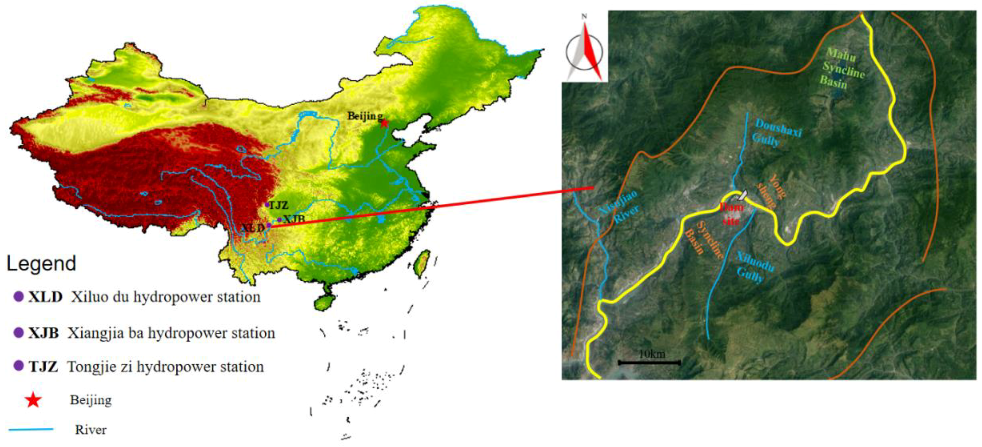
Take the Xiluodu Hydropower Station as an example. The Xiluodu Hydropower Station is located on the main stream of Jinsha River in Leibo County of Sichuan Province and Yongshan County of Yunnan Province. The location of the study area is shown in Figure 3. The reservoir has a normal water level of 600 m. The Xiluodu Hydropower Station cooperates with the Three Gorges Project to improve the flood control capacity of the middle and lower reaches of the Yangtze River, which give full play to the comprehensive benefits of the Three Gorges Project. Besides, it promotes the development of the western region and realizes the sustainable development of the national economy. The river bedrock and the valley slopes on both sides of the dam site are composed of Emeishan basalt (P2β) of the Upper Permian, and the Maokou limestone (P1m) of the Lower Permian is buried 70 m below the dam foundation. The research suggests that the patterns of valley and foundation deformation caused by reservoir impoundment processes are closely related to the groundwater flow in the aquifers. Therefore, it is of great significance to calculate the influence of reservoir impoundment on groundwater level [24].

3.2. Representation of River Level

In the analytical solution, it is necessary to generalize the river level in different forms in order to calculate the unsteady flow in the unconfined aquifer caused by the river level variation and compare the piecewise-linear model with the traditional piecewise-constant step model proposed in this article. Consider the water level monitoring data of Jinsha River in 1995 as original data to fit. As shown in Figure 4, the river level variation in a hydrological year presents seasonal variation. The rise of river level is concentrated in June–September, during which there is obvious fluctuations of water level likely related to seasonal rainfall. On the whole, the water level variation is complex, and it is difficult to express its change with simple functions. The river level is divided into 7 and 17 segments by piecewise-linear and piecewise-constant step approximations. The more segments are divided, the closer the approximate values are to the original data. The time segments are automatically divided by the written program according to the input accuracy requirements, not manually partitioned. The piecewise-linear approximation proposed in this paper is used to generalize the river level, which can not only reflect the water level change trends but also show the characteristic water level and corresponding time points. However, the traditional piecewise-constant step approximation can only represent the overall change characteristics and ignores the stage change characteristics. This demonstrates that, for the cases where river level variations are better represented by piecewise-linear approximation, as river level variations may not be adequately expressed by a relatively small number of step segments, the piecewise-constant step approximation for representing river level transients is not always sufficient to accurately represent the observed data.

3.3. Model Calculation

In order to study the unsteady flow of the unconfined aquifer caused by the river level variation, it is necessary to analyze and determine the hydrogeological parameters of the basalt in the bank slope. Reasonable values of the hydrogeological parameters are very important for the reliable analysis of the calculation results. The hydraulic conductivity of the basalt area measured by field tests of the Xiluodu Hydropower Station ranged from 0.06 m/d to 2.70 m/d, in which the hydraulic conductivity and the porosity of rock mass were small. The average hydraulic conductivity and porosity (K = 0.90 m/d, n = 0.03) after excavation were selected to calculate and specific yield was approximated as porosity. The initial thickness of the unconfined aquifer was H = 153 m, and the horizontal extension distance of the study area was 7.9 km.
At 85.7 m and 371.4 m away from the river valley, the groundwater level at the selected location was calculated by piecewise-linear and piecewise-constant step models, respectively. At the same time, the dynamic observed data of the water level at the corresponding long-term observation wells X35 and X50 were used to verify the accuracy of the two models. The calculated results are shown in Figure 4. It is obvious from the fitting degree of the calculated results and the long-term observation data that the groundwater level calculated by the piecewise-linear model was closer to the dynamic observed data of the long-term observation well. In order to quantify the calculation accuracy of the two models, the RMSE (root mean square error) and RE (relative error) were used to represent the deviation between the calculated and the observed values, which could be expressed with Equations (11) and (12) and the calculated results as shown in Table 1. The error analysis showed that the more segments were divided, the higher the calculation accuracy was, and the calculation accuracy of the piecewise-linear model was higher than that of the piecewise-constant step model.
R M S E = 1 n i = 1 n ( H c , i H m , i ) 2
R E = 1 n i = 1 n   | H c , i H m , i | H m , i × 100 %
where Hc,i denotes the calculation value of groundwater level at the ith time point, Hm,i denotes the corresponding monitor data, and n is the total number monitored.
In general, the groundwater dynamic in the long-term observation well was basically consistent with the river level dynamic, which represents good synchronization. The main reason is that the distance between the selected long-term observation well and the river valley was relatively short compared with the whole study area, and the signal damping phenomenon was not obvious. However, the long-term observation wells X35 and X50, which are located close to and far from the river valley, respectively, performed different response degrees of groundwater level to river level variation. Compared with the river level values and the groundwater level observed data, with the distance increasing, the amplitude of groundwater level variation decreased, and the groundwater level variation delay phenomenon in the X50 was more notable than that in the X35, which is related to the flow resistance of the rock. From the calculation results, the errors of X50 were greater than those of X35, which may be due to the selection of hydraulic parameters. For the convenience of model calculation, we chose the same hydraulic diffusivity in an unconfined aquifer to calculate the groundwater dynamic at different locations from the valley. However, the hydraulic diffusivity in an unconfined aquifer near a river valley is generally larger than that far from valleys, which is related to the good permeability of rock masses and the fast discharge of groundwater near the river valley. Therefore, the same hydraulic diffusivity in the unconfined aquifer selected may affect the accuracy of groundwater level calculations at different locations.

3.4. Prediction of Groundwater Level Fluctuation Caused by Reservoir Water Level Variation

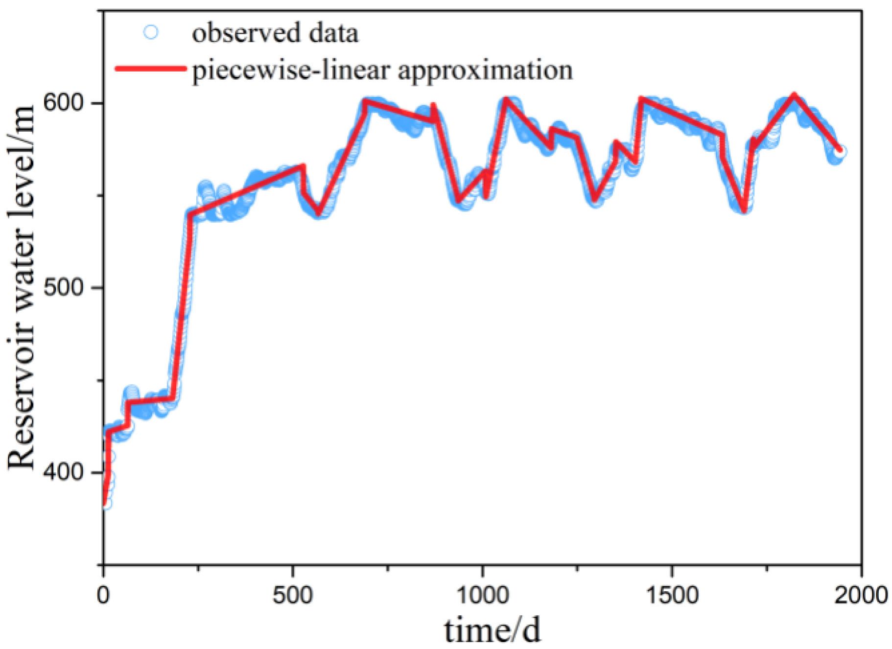
From the model calculation results and groundwater dynamic data in the long-term observation well, the piecewise-linear model has a high reliability in calculating groundwater flow caused by the boundary water level variation. This example has shown that the analytical model can be used to represent the flow with sufficient accuracy. The Xiluodu Hydropower Station has been impounded since 30 October 2012. The initial river level was 383.45 m. In November 2014, the impoundment had reached the normal water level of 600 m, and in the observed data of the reservoir water level until 26 February 2018, the water level fluctuated periodically. Taking the initial time of 30 October 2012 and the end time of 26 February 2018 for 1943 days, the reservoir water level variation was generalized by a piecewise-linear approximation, which was divided into 43 continuous linear segments, as shown in Figure 5.
We analyzed the unsteady flow of unconfined aquifer caused by the reservoir water level variation according to the piecewise-linear approximation proposed in this paper. Four selected time nodes were 9 February 2013, 16 March 2014, 29 July 2015, and 14 February 2018 corresponding to 100, 500, 1000, and 1900 d (based on the initial time of impoundment) to analyze the distribution of the water level at each point in the study area. At the same time, groundwater level variations with time were considered at 0.2, 0.5, 1.0, 2.0, 3.0, 5.0, and 7.9 km (the water barrier boundary) away from the reservoir bank, as shown in Figure 6. A rising reservoir water level will recharge the unconfined aquifer and cause a long-term and wide-ranging impact. The explanation of the long-term characteristic is that basalt has good integrity, a large thickness, a compact structure, low permeability, and most are dry under natural conditions. In addition, the hydraulic response of groundwater in the unconfined aquifer mainly depends on gravity, supplemented by pressure transfer. When river water recharges unconfined water in basalt strata, the developed joints, interlayer, and internal shear zones are saturated firstly. The process of mountain saturation is extremely slow, and the corresponding water level rise is slow, so the river water will recharge the unconfined aquifer for a long time. The wide range was due to the broad horizontal extension of basalt stratum and the low, gentle, natural groundwater level of unconfined water. What is more, after reservoir impoundment, there was a large distribution area, where the unconfined surface elevation of the mountain body was smaller than the reservoir’s normal water level.
At the same time, the water level decreased gradually as it extended from the reservoir bank to the side away from that, showing obvious damping of gravity water release. The unconfined water surface advanced continuously as time went on. When the time was 100 d, the transfer distance of groundwater level fluctuation caused by the reservoir water level variation was 4200 m, which is shown in the A point coordinates (4200, 383.45); when the time was 500 d, it had been transferred to the impervious boundary, where the water level was 383.56 m; when the time was 1000 d, the water level at the impervious boundary was 390.33 m; when the time was 1900 d, the water level at the impervious boundary is 434.25 m. The analyzed data show that the water level rises slowly and never equals the reservoir water level, which indicates that the unconfined aquifer response to the reservoir water level variation has obvious damping characteristics. At time 0 d, the groundwater level is at the initial time. According to the existing survey data, at the initial time, the fluctuation range of the groundwater level in the whole study area was very small, only 0.5 m, so the groundwater level at this time was approximately a plane, with a value of 383.45 m.
Comparing the time-varying curves of groundwater levels at 0.2, 0.5, 1.0, 2.0, 3.0, 5.0, and 7.9 km away from the reservoir bank, the groundwater level at the same location showed an overall upward trend with time. Zero kilometer indicates the reservoir water level variation. At 0.2, 0.5, and 1.0 km, the groundwater level fluctuated obviously with time, showing a good synchronization with the reservoir water level variations, although the increase was less than that. At 2.0 km, there was slight groundwater level fluctuation. With the distance increasing, the fluctuation of the groundwater level nearly disappears, reduced gradually at 3, 5 and 7.9 km, showing only an increase of the water level. In addition, when the reservoir water level changed periodically, the damping of the hydraulic response in the unconfined aquifer was also reflected in the phase difference between the groundwater level and the reservoir water level. When the reservoir water level changed from ascending to descending (descending to ascending), the groundwater level at a certain position away from the bank slope kept ascending (descending) for a period of time, and then, it began to descend (ascend), which indicates the existence of a certain phase difference. The farther away from the bank slope, the bigger the phase difference is, and it cannot even reflect the fluctuations of the reservoir water level. It can be seen that the groundwater level changed greatly near the bank slope, and the hydraulic damping effect was smaller, which can reflect the change characteristics of the reservoir water level. However, the variation range of groundwater level was smaller far from the bank slope, the hydraulic damping effect had greater influence, and the change characteristics of the reservoir water level attenuated accordingly. It is worth to point out that this system behavior (phase difference, damped fluctuation) was in line with other studies [25]. Since the model is assumed to be an impervious boundary, the limit value of the groundwater level variation at each point in the unconfined aquifer will not exceed the maximum rise value of the reservoir water level. The steady state flow of groundwater was not being achieved after 2000 days.

4. Results and Discussions

The analytical solutions of groundwater level versus time and distance are developed to investigate the impacts of the boundary water level approximation, models accuracy, and damping effects in an unconfined aquifer. The mathematical model assumes that rainfall, aquifer recharge, extractions, and base flow discharge are zero, which may be different from the actual situation. This paper mainly discusses the influence of boundary water level on groundwater flow. In order to simplify the analytical solution, other recharge and discharge values are considered as zero.

4.1. Effect of Boundary Water Level Approximation

Analytical solutions are derived to study the groundwater flow in this article. The analytical solutions, different from numerical simulation, and the boundary conditions could not be represented as discrete data points. However, the original time resolution of the river level versus time series could not be represented with a normal function. Therefore, we applied the piecewise-linear approximation to generalize the river level variation, so it could be shown with an expression. Linear segments (7 and 17) were divided in the river level, as shown in Figure 4a,b, and the results indicated that the higher the time resolution, the smaller the deviation between the calculated values and the original data.

4.2. Effect of Models Accuracy

Figure 4 displays the curves of groundwater level versus time for long-term observation wells X35 and X50 with piecewise-linear and piecewise-constant step approximations. Table 1 shows the error analysis with different approximations. Both demonstrate that the accuracy of the piecewise-linear approximation was higher than that of the piecewise-constant step with the same time resolution.

4.3. Effect of Damping in the Unconfined Aquifer

Figure 6 presents the groundwater response lags behind the reservoir water level variation. The further away from the reservoir bank, the more obvious the time delay. It is obvious that the filling of the reservoir overrides this surface subsurface water interaction effect in the first 700 days. In addition, the groundwater level has not achieved a steady state, even after 2000 days, and the maximum water level at 7.9 km was far below the reservoir level in the simulation period. If the reservoir water level still changes periodically and the simulation time is extended, the water level at the impervious boundary could reach to the reservoir’s impoundment level at about 6000 days from the initial time, which is about the year 2030.

5. Conclusions

The river level usually presents a non-linear continuous change over time, which is different from the instantaneous rise or piecewise-constant step variation of the water level. According to the river level variation characteristics, a piecewise-linear approximation is proposed to generalize the river level variation. Based on the actual situation, the other side of the study area is set as an impervious boundary, and the analytical solution of groundwater unsteady flow caused by the river level variation is derived.
Results were compared with the traditional piecewise-constant step model to illustrate the calculation accuracy. Taking the Xiluodu Hydropower Station as an example to validate the method proposed in this paper, the piecewise-linear approximation values to the boundary water level are closer to the actual water level variation process, which can reflect the variation characteristics. The calculation accuracy of the piecewise-linear model is higher than that of the piecewise-constant step model through the verification of groundwater dynamic monitor data in the long-term observation well. The response of the groundwater level dynamic in an unconfined aquifer to the reservoir water level variation has obvious damping, which demonstrates that the farther away from the bank slope, the more obvious the time delay. The piecewise-linear approximation of the time-varying boundary water level can also be applied to predict the hydraulic response in the confined aquifers and aquitards. It should be made clear that this exercise is only relevant for the analytical solutions. Numerical models can only use the boundary condition time series on the resolution of the model.
Based on the groundwater level variation obtained, we will estimate the surface-subsurface water exchange and study the influence of rainfall, aquifer recharge, extractions, and base flow discharge on the groundwater level and quantity in further work.

Author Contributions

Conceptualization, Y.X. and Z.Z.; methodology, Y.X.; software, Y.X., M.L. and C.Z.; validation, Z.Z., M.L. and C.Z.; formal analysis, Y.X.; investigation, Y.X.; resources, Z.Z.; data curation, Y.X.; writing—original draft preparation, Y.X.; writing—review and editing, Y.X. and Z.Z.; visualization, Y.X.; supervision, Z.Z. All authors have read and agreed to the published version of the manuscript.

Funding

This research was funded by the National Natural Science Foundation of China, grant number No. 41572209, and China Three Gorges Corporation, grant number No. 20188019316.

Conflicts of Interest

The authors declare no conflict of interest.

References

  1. Lischeid, G. Drivers of water level fluctuations and hydrological exchange between groundwater and surface water at the lowland River Spree (Germany): Field study and statistical. Hydrol. Processes 2009, 23, 2117–2128. [Google Scholar]
  2. Mclachlan, P.J.; Chambers, J.E.; Uhlemann, S.S.; Binley, A. Geophysical characterisation of the groundwater-surface water interface. Adv. Water Resour. 2017, 109, 302–319. [Google Scholar] [CrossRef] [Green Version]
  3. Chen, J.W.; Hsieh, H.H.; Yeh, H.F.; Lee, C.H. The effect of the variation of river water levels on the estimation of groundwater recharge in the Hsinhuwei River, Taiwan. Environ. Earth Sci. 2010, 59, 1297–1307. [Google Scholar] [CrossRef]
  4. Zhou, Z.; Wang, J. Groundwater Dynamics; Science Press: Beijing, China, 2013. [Google Scholar]
  5. Rushton, K. Representation in regional models of saturated river-aquifer interaction for gaining/losing rivers. J. Hydrol. 2007, 334, 262–281. [Google Scholar] [CrossRef]
  6. Goerlitz, D.F.; Troutman, D.E.; Godsy, E.M.; Franks, B.J. Migration of wood-preserving chemicals in contaminated groundwater in a sand aquifer at Pensacoia, Florida. Environ. Sci. Technol. 1985, 19, 955–961. [Google Scholar] [CrossRef]
  7. Zhao, M.L. Finite element numerical simulation of two-dimensional ground water solute migration question. Adv. Mater. Res. 2011, 301–303, 352–356. [Google Scholar] [CrossRef]
  8. Luo, Z.; Yang, L.; Li, Z.; Wang, J. Three-dimensional numerical simulation for immersion prediction of left bank of Songyuan reservoir project. Trans. Chin. Soc. Agric. Eng. 2012, 28, 129–134. [Google Scholar]
  9. Celia, M.A.; Bouloutas, E.T.; Zarba, R.L. A general mass-conservative numerical solution for the unsaturated flow equation. Water Resour. Res. 1990, 26, 1483–1496. [Google Scholar] [CrossRef]
  10. Li, M.; Zhou, Z.; Yang, Y.; Xin, Y.; Liu, Y.; Guo, S.; Zhu, Y.; Jin, D. Immersion assessment and control of the right bank of Xingan navigation and power junction. J. Hohai Univ. Sci. 2018, 46, 203–210. [Google Scholar]
  11. Pinder, G.F.; Sauer, S.P. Numerical simulation of flood wave modification due to bank storage effects. Water Resour. Res. 1971, 7, 63–70. [Google Scholar] [CrossRef]
  12. Yuan, F.; Lu, Z. Analytical solutions for vertical flow in unsaturated, rooted soils with variable surface fluxes. Vadose Zone J. 2005, 4, 1210–1218. [Google Scholar] [CrossRef]
  13. Ferris, J.G.; Knowles, D.B.; Brown, R.H.; Stallman, R.W. Theory of Aquifer Tests; US Geological Survey: Denver, CO, USA, 1962.
  14. Mahdavi, A. Transient-state analytical solution for groundwater recharge in anisotropic sloping aquifer. Water Resour. Manag. 2015, 29, 3735–3748. [Google Scholar] [CrossRef]
  15. Su, N. The fractional Boussinesq equation of groundwater flow and its applications. J. Hydrol. 2017, 547, 403–412. [Google Scholar] [CrossRef] [Green Version]
  16. Wu, D.; Tao, Y.; Lin, F. Application of unsteady phreatic flow model and its solution under the boundary control of complicated function. J. Hydraul. Eng. 2018, 6, 725–731. [Google Scholar]
  17. Zhang, W. Calculation of Unsteady Groundwater Flow and Evaluation of Groundwater Resources; Science Press: Beijing, China, 1983. [Google Scholar]
  18. Bansal, R.K. Approximation of surface–groundwater interaction mediated by vertical streambank in sloping terrains. J. Ocean Eng. Sci. 2017, 2, 18–27. [Google Scholar] [CrossRef] [Green Version]
  19. Mishra, P.K.; Vessilinov, V.; Gupta, H. On simulation and analysis of variable-rate pumping tests. Groundwater 2013, 51, 469–473. [Google Scholar] [CrossRef]
  20. Stewart, G.; Watt, H.U.; Wittmann, M.J.; Meunier, D. After flow measurement and deconvolution in well test analysis. In Proceedings of the SPE Annual Technical Conference and Exhibition, San Francisco, CA, USA, 5–8 October 1983. [Google Scholar]
  21. Zhuang, C.; Zhou, Z.; Zhan, H.; Wang, G. A new type curve method for estimating aquitard hydraulic parameters in a multi-layered aquifer system. J. Hydrol. 2015, 527, 212–220. [Google Scholar] [CrossRef]
  22. Lee, J.; Wilson, D. Polyhedral methods for piecewise-linear functions I: The lambda method. Discret. Appl. Math. 2001, 108, 269–285. [Google Scholar] [CrossRef] [Green Version]
  23. Sontag, E.D. Nonlinear Regulation: The Piecewise Linear Approach. IEEE Trans. Automat. Control 1981, 26, 346–358. [Google Scholar] [CrossRef]
  24. Zhou, Z.; Li, M.; Zhuang, C.; Guo, Q. Impact factors and forming conditions of valley deformation of Xiluodu Hydropower Station. J. Hohai Univ. Sci. 2018, 46, 31–39. [Google Scholar]
  25. Becker, B.; Jansen, M.; Sinaba, B.; Schüttrumpf, H. On the modeling of bank storage in a groundwater model: The April, 1983, flood event in the Neuwieder Becken (Middle Rhine). J. Water 2015, 7, 1173–1201. [Google Scholar] [CrossRef] [Green Version]
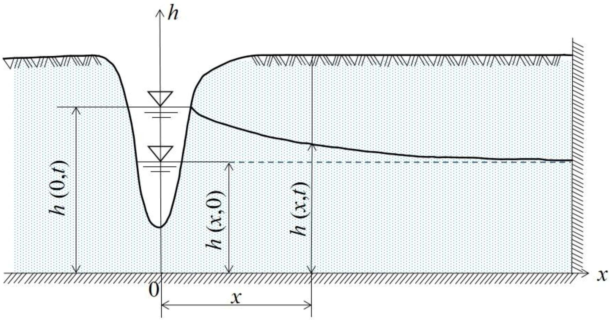
Figure 1. Conceptual model of groundwater flow near the riverbank.
Water 12 00075 g001
Figure 2. River level variations for sinusoidal (g1), exponential (g2), and random (g3) characteristics with piecewise-linear approximation.
Water 12 00075 g002
Figure 3. Map showing the geographic location of the study area.
Water 12 00075 g003
Figure 4. Riverhead variation in 1995 is divided into 7 segments (a) and 17 segments (d), respectively with piecewise-linear and piecewise-constant step approximations; i is the segments; and calculated results of groundwater-level variation for long-term observation wells X35 (b,e) and X50 (c,f) with piecewise-linear and piecewise-constant step approximations for different segments.
Water 12 00075 g004
Figure 5. Reservoir water level duration curve represented with piecewise-linear approximation.
Water 12 00075 g005
Figure 6. Groundwater-level fluctuation curves at different points in study area (a) and groundwater-level duration curves (b) in the unconfined aquifer.
Water 12 00075 g006
Table 1. Root-Mean-Square Error (RMSE) and Relative-Error (RE) between observed and calculated data with Piecewise-Linear (Columns 3 and 4) and Piecewise-Constant Step (Columns 5 and 6).
Linear ApproximationStep Approximation
RMSERERMSERE
i = 7X351.740.00332.330.0046
X502.350.00472.630.0053
i = 17X351.500.00281.810.0036
X501.820.00362.520.0049