Abstract
The Molise region (southern Italy) fronts the Adriatic Sea for nearly 36 km and has been suffering from erosion since the mid-20th century. In this article, an in-depth analysis has been conducted in the time-frame 2004–2016, with the purpose of discussing the most recent shoreline evolution trends and individuating the climate forcings that best correlate with them. The results of the study show that an intense erosion process took place between 2011 and 2016, both at the northern and southern parts of the coast. This shoreline retreat is at a large extent a downdrift effect of hard protection systems. Both the direct observation of the coast and numerical simulations, performed with the software GENESIS, indicate that the shoreline response is significantly influenced by wave attacks from approximately 10° N; however, the bimodality that characterizes the Molise coast wave climate may have played an important role in the beach dynamics, especially where structural systems alternate to unprotected shore segments.
1. Nature of the Problem
The study of shoreline change, and the prediction of its future development, are essential for integrated coastal zone management. Nowadays, many shorelines of the world are suffering from a deficit of sand, which may lead to a gradual or fast coastline retreat; of course, this represents a leading concern to coastal scientists and planners.
In principles, beach erosion may result from either natural or anthropogenic causes; natural changes are generally difficult to interpret, and can be often attributed to a simple long-term fluctuation of the littoral system, as well as to the rise of the sea level [1]. On the other hand, anthropogenic causes are easily individuated, and include a reduction in the natural sand supply due to up river reservoir construction, and the presence of ports or navigational entrances, the structures of which (e.g., jetties) tend to interfere with longshore sediment transport.
Various approaches exist for beach stabilization, that can be broadly classified as structural (or hard) and non-structural (or soft). Purely non-structural approaches are limited to beach nourishment, which consists of introducing a given amount of good quality sand in the nearshore, so to counteract the misbalance between sediment inputs and outputs.
On the other hand, hard approaches include a number of variants, such as bank protection (essentially revetments and seawall), detached breakwaters and groins; structures interact with incoming waves via a number of complex hydrodynamic processes, including wave transmission, wave set-up, wave reflection and wave overtopping, which makes the prediction of shoreline response rather uncertain [2]. For this reason, all those processes have been intensively researched in recent decades, mostly through physical and numerical experiments [3,4,5,6,7,8,9,10,11,12,13]. However, a common feature of structural approaches is that they do not supply new sand to the littoral system, and accordingly if they succeed in locally widening the beach, they also inevitably induce erosion on the adjacent stretches of coast.
Thus, unsurprisingly, a number of literature studies document the negligible or deleterious effects of structural solutions in the long term; this especially occurs when structures are built in emergency conditions, as argued by Masria et al. [14] for the Mediterranean coasts. Among the other examples, Dean et al. [1] discussed the case of Palm Beach, Florida, where nearly 82,000 m3 of sand were lost (over three years) after the placement of an experimental proprietary submerged breakwater of 1260 m in length.
The uncertainty related to structural solutions have sometimes led governments to give up on them, leaving beach nourishments as the sole alternative for beach erosion control. This is the case, for example, of the Romagna Riviera (Italy, North Adriatic Sea), where after having used breakwaters and groins with mixed success between late 1950s and late 1970s, the 1981 Regional Coastal Plan eventually prohibited the construction of new structures; since then, over one million cubic meters of sand has been used for repeated beach nourishment interventions [15].
2. Research Aims and Outline
This article deals with the case of the Molise coast, Southern Italy, which fronts the Adriatic Sea and is located nearly 300 km south of the Romagna Riviera.
In the frame of a collaboration between the University of Molise and the University of Napoli “Federico II”, a shoreline change study was carried out, aiming to:
- Analyze the most recent trends of Molise coast evolution;
- Investigate the possible relationships between wave directions and shoreline response.
The reference time window is the period 2004–2016, which updates previous literature studies [16]; according to the definition originally introduced by Crowell et al. [17], the present analysis can be conventionally referred to as a “Mid-term study”.
Differently from the approach followed in early research e.g., [16,18,19], in this paper attention was drawn to selected “hot spot” areas, and for each of them, the possibility of generating forcings are discussed. Then, a hypothesis was formulated about the existence of a dominant wave attack for littoral transport, which we will refer to as “equivalent wave” (EW), and its degree of correlation with the coastline evolution is examined.
In this regard, it is worth highlighting that the “Equivalent Wave Concept” is widely (and trustily) used in the field of practical coastal engineering, in spite of it lacking a firm theoretical basis. Thus, present research basically represents the first systematic attempt at investigating the explanatory power of the EW concept. In the following, this task is accomplished either numerically, employing the one line model GENESIS [15], or via physical considerations.
The results presented below apply to the whole Molise coast and are mainly of a qualitative nature; a quantitative comparison for a more restricted reach, is instead discussed in a further study submitted to this Special Issue [20].
The paper is organized as follows. After an overview of the Molise coast evolution and the related literature (Section 3), the GENESIS model is briefly reviewed in Section 4. Then, the wave climate in the study area is examined in Section 5 and the shoreline change process during the period 2004–2016 is illustrated in Section 6. Finally, the “equivalent wave” concept and its possible applications are dealt with in Section 7.
3. Study Area and Early Literature
The Molise coast extends for 36 km and is prevalently exposed to waves coming from the northern quadrants (Figure 1). The rocky cliff of Termoli promontory splits the coastline into two reaches. One stretches from the harbor of Marina Sveva to the promontory of Termoli; the second reach extends between the Termoli harbor and the Saccione stream mouth and includes the harbor of Marina di Santa Cristina (Figure 1).
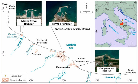
Figure 1.
Molise coast with the main harbor location.
Molise beaches are composed of medium sand (average diameter 0.26 mm) and are characterized by a very gentle foreshore (slope less than 1% between 0 and 10 m below the Mean Water Level, MWL). The average berm height is 2.0 m above the MWL [16,18].
Starting from the mid-20th century, a significant erosion has been taking place, which has been recognized to be caused to a large extent by the restrictions imposed to the river flows and the consequent decrease in sediment delivery to the coast [16,18,19]. In particular, the S. Salvo check-dam, built across the Trigno River during the period 1954–1977, and the Ponteliscione dam, built across the Biferno River between 1965 and 1977, have strongly contributed to channel incision and narrowing [21] and deprived the coastal sedimentary budget of significant volumes; De Vincenzo et al. [22,23] estimated that from 1965 to 2007, nearly 4.4 × 10⁶ m3 of sediments have accumulated within the Ponteliscione dam reservoir.
The response to progressive shoreline erosion was of a fully “structural” nature and nowadays nearly 62% of the coast is covered by hard protection measures; structures include mainly segmented systems of detached breakwaters, either submerged or emerged, and groins.
The evolution of the Molise coast has been intensively investigated in recent decades. Among the most relevant research, Aucelli et al. [24] analyzed the 1954–2000 shoreline changes of a 10 km long reach astride the Termoli promontory. The authors performed an accurate analysis of both wind and wave climates and concluded the main wave forcings to come from either the NW or NE. The maximum erosion risk was localized in the “densely structured” area neighboring the Biferno River mouth. Finally, based on the shoreline orientation of the examined coastal segment, a net NW to SE littoral drift was postulated.
Recently, Rosskopf et al. [16] extended the analysis to the whole Molise coastline and widened the reference time interval to 1954–2014. The coast was partitioned into nine physiographically homogeneous sub-reaches, the length of which ranged between 2 and 7 km; then, the average rate of shoreline change was calculated for the different time windows.
The authors warned that in spite of the substantial stability observed during the period 2004–2014, a new erosion process might be arising either at the northern or the southern part of the coast. Although a prevailing NW to SE littoral drift was inferred, a number of possible inversion areas were indicated, such as at the Trigno river mouth or right at the south of the Termoli harbor. Finally, a more in-depth knowledge of wave forcing was auspicated for future research work.
4. Overview of GENESIS Model
GENESIS (Generalized Model for Simulating Shoreline Changes) is a numerical modeling system, simulating shoreline evolution by spatial and temporal differences in longshore sand transport [25]. Despite being known worldwide, some of its characteristics are outlined below to facilitate the comprehension of Section 6.
GENESIS integrates the one-line contour equation (OCL), which expresses the conservation of sand volume; the leading hypotheses adopted are that the beach profile moves in parallel to itself and littoral transport is included between the berm height, DB, and the depth of the closure, Dc [26]. The OCL reads:
where beside the already introduced quantities:
- y (x,t) is the cross-shore coordinate of the shoreline at the alongshore position x and time t;
- Q is the littoral drift rate.
As is widely known, the beach change process is influenced by many environmental factors; these include wave propagation and breaking, nearshore currents activated by the release of wave momentum in the surf-zone and, finally, sediment transport. However, in the model the horizontal circulation that actually moves sediments is not simulated; the littoral drift rate is then empirically related to wave and sand characteristics, according to the formula:
in which:
- Hs is the significant wave height;
- cg is the group celerity;
- The subscript “b” denotes incipient breaking conditions;
- θ is the angle between the wave front and the shore;
- tanβ is the average beach slope between the shoreline, down to a depth D = 2H;
- K1 and K2 are transport coefficients;
- C1 and C2 are coefficients related to the sediment properties.
The first term at the right-hand side of Equation (2) corresponds to the well known Coastal Engineering Research Center (CERC) formula [27], and accounts for longshore sand transport produced by obliquely incident breaking waves. The second term simulates the effect of an alongshore gradient in breaking wave height, which may take place for a considerable length of beach in the vicinity of diffractive structures.
Breakwaters (both transmissive and non-transmissive), jetties and groins are easily implemented in GENESIS, but only structures located seaward the breaker-line are assumed to produce diffraction. Diffractive structures segment the calculation domain into energy windows, penetrable by waves; accordingly, the shoreline is divided into several “sand transport calculation domains”, communicating with each other via sand bypassing and transmission.
As far as lateral boundary conditions are concerned, three constraint types can be used, and namely:
- “Pinned” if a portion of the beach is assumed to not move appreciably in time;
- “Gate” if the movement of sand alongshore is interrupted, partially or completely;
- “Moving” if the modeler specifies the rate of shoreline change on an end of the calculation grid.
5. Wave Climate Analysis
Data acquired by a directional wave buoy located in the offshore waters fronting the town of Ortona, 56 km north the mouth of Trigno river, were used to infer the wave climate at Molise coast (Figure 2). The device was anchored at a depth of 70 m below the low tide level, at a latitude of 42°24′54.0″ N and a longitude of 14°30′20.99″ E.
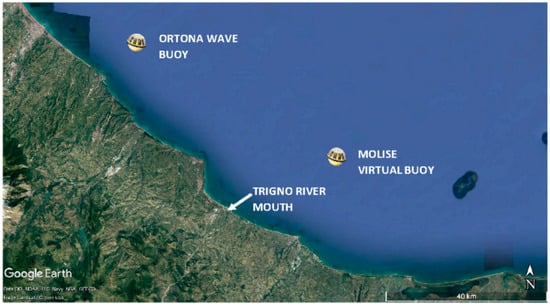
Figure 2.
Ortona wave buoy and “virtual” wave buoy at the Molise coast.
Significant wave height, Hs, peak period, Tp, and azimuth of the mean wave direction, α, were recorded during the period 1989–2012, at an average interval of 3 h. Wave heights and periods were adjusted to the sea offshore the Molise coast (“virtual buoy” in Figure 2), according to the relationships originally introduced by Hasselmann [28] in the frame of the JONSWAP project. Assuming the same wind to blow at both the “real” and “virtual” buoy location, it is readily obtained that [29]:
where F indicates the “effective fetch” [30]. Note that, consistently with Hasselmann [28], the mean direction of the waves was assumed to coincide with that of the wind.
The histogram of the wave direction for angular sectors of 22.5° N is displayed in Figure 3, where the offshore directed waves have been removed for the sake of clearness.
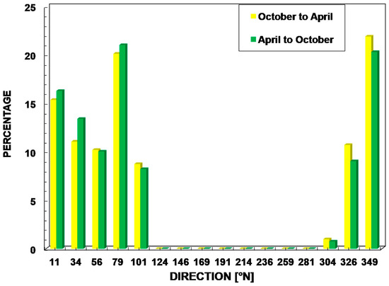
Figure 3.
Histogram of the wave directions. Onshore directed angles are removed.
The graph exhibits two well defined modes, which were shown to be seasonally invariant; one is around 350° N and coincides with the NNW dominant direction indicated by Aucelli et al. [24]; the other is close to 80° N, whereas the authors indicated 23° N.
The reason for this apparent inconsistency is because waves from ENE-E have a lower height; hence, they bring forth less energy. This is shown in Figure 4, where along with the mean wave height, the 90th percentile of the directional wave height distribution is also reported. The graph indicates that the highest waves tend to come from 0°–45° N, in accordance with Aucelli et al. [24], with a maximum in the sector 0°–22.5° N.
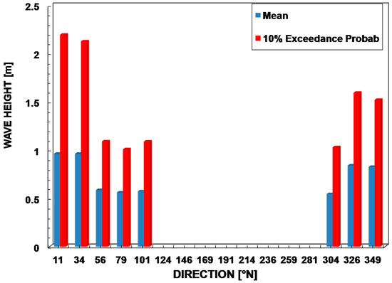
Figure 4.
Directional distribution of mean and 90th percentile wave height.
The significant wave height was exceeded by 12 h a year (HE), and has been estimated for each angular sector after fitting a two-parameter Weibull distribution to the wave data. An average value of 4.08 m was obtained keeping only the onshore directed angles; this value was used for the depth of the closure calculation (Dc ≈ 2 HE) according to Hallermeier [26].
The joint Hs-Tp distribution (e.g., Figure 5) revealed a small wave height (less than 1 m) to have a modal peak period included between 3 and 6 s, whereas for the waves between 1.5 and 4.5 m, the modal Tp progressively moves to the interval 6–9 s. Finally, the period of the largest waves (larger than 4.5 m) is invariably included between 9 and 12 s. The overall mean peak period (direction independent) equals 5.08 s.
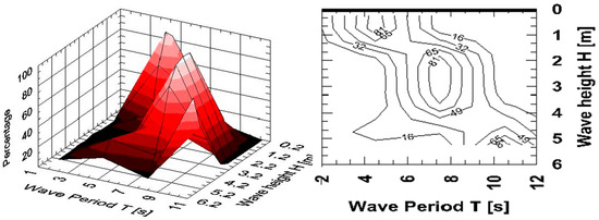
Figure 5.
Joint distribution (Hs-Tp) for the angular sector 0–22.5° N. Left panel: 3D distribution. Right panel: contour lines.
6. Analysis of Shoreline Change
A shoreline change analysis was carried out, by comparing the Molise coastline position in 2004, 2011, 2014, and 2016. As mentioned above, according to Crowell et al. [17], the present study can be considered a “medium-term” investigation.
6.1. Approach
As shown in Table 1, data come from the digitalization, in the ArcGis environment, of photograph reliefs from different sources.

Table 1.
Summary of the shoreline data.
The shoreline location has been assumed to coincide with the instantaneous waterline, which is reasonable in virtue of the low tidal environment [16]. Rough data has been linearly interpolated, and finally re-sampled at a 10 m interval.
Table 1 also reports the uncertainties related to the digitalization procedure (last column, RMS), being the other sources of inaccuracy, such as georeferencing, airphoto, etc., virtually absent; RMS values are consistent with those indicated by Hapke et al. [31] and Crowell et al. [17].
It is worth mentioning that digitalization uncertainties are essentially generated by human factors and measurement routine; accordingly, they can be considered as “chance” or “stochastic” errors, to be treated in the frame of the classical theory of errors [32,33].
Thus, each shoreline measurement can be thought as the sum of the “true” shoreline position, plus a random component, which we will model as a Gaussian random variable with zero mean and a standard deviation equal to RMS (Table 1).
Moreover, since each digitalization has been performed independently of the others, the random components can be considered as mutually independent from a statistical point of view.
The linear regression rate (LRR) has been used as an indicator of the rate of shoreline change; it represents the slope of a least-square straight-line, fitted through the shoreline positions at the various available times. As argued in Douglas and Crowell [34] and Maiti and Bhattacharya [35], the use of least square fitting significantly reduces either the effect of random errors or that associated with other cyclical factors, such as tidal fluctuations.
However, differently from previous literature works, here the following procedure has been adopted:
- The LRR at a given horizontal axis, x, is calculated after gathering all the data falling within a centered window of 40 m width. The window, is then progressively moved forward;
- The obtained slope, say sx, is tested for significance at a 95% probability level, according to the well established linear regression theory (see [36]);
- Whenever the test is not satisfied, LRR is finally set to zero.
Note that the point c. implies:
The use of a moving window allows collecting a larger number of points, making the statistical test less unstable. Moreover, the procedure keeps holding its meaning (at least up to certain extent), even when comparing two shorelines only.
Finally, it is worth highlighting that the 95% probability level at the previous point b, has been chosen with the purpose of also including the uncertainties related to the interpolation/resampling procedure.
From the LRR(x) function, accretion and erosion areas have been identified as those segments of coast where the shoreline change rate exceeds a certain limit value, say vLIM, and remains above it for a minimum length, lLIM.
For the scope of the regional analysis here presented, lLIM has been set to 500 m, whereas vLIM has been conveniently related to the uncertainties of the measurement process. The approach here employed is similar to that suggested, among the others, by Hapke et al. [31].
After invoking the gaussianity and independency of the random errors related to each shoreline measurement, it follows, from the theory of probability, that the error related to the difference between the two shoreline measurements at different times, say is in turn a Gaussian random variable, with zero mean and variance [36]:
Consequently, we have that at a 95% probability level the error is included in the interval [36]:
Thus, if the “true” position of the shoreline remains unvaried in the interval , measurement errors may generate a fictional rate of change, which is included in the interval:
with 95% probability.
Hence, it seemed reasonable to assume , that is to say that a shoreline segment is subject to a significant evolution if its rate of change overcomes that possibly created by measurement errors.
Values of vLIM for the intervals 2004–2016, 2004–2011, 2011–2016 and 2014–2016 are reported in Table 2.
Table 2.
Values of vLIM for different time windows.
6.2. Results
Figure 6 shows the 2004–2016 LRR function, whereas Figure 7 displays the corresponding erosion/accretion areas. In both the graphs, the alongshore coordinate, x, is oriented from NW to SE; horizontal dashes indicate detached breakwaters, whereas vertical dashes represent groin fields. From the inspection of Figure 7, it is easily observed that:
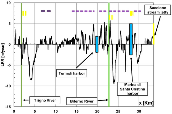
Figure 6.
Linear regression rate (LRR) function during the period 2004–2016. Horizontal dashes indicate the detached breakwaters; the vertical dashes indicate groin fields.
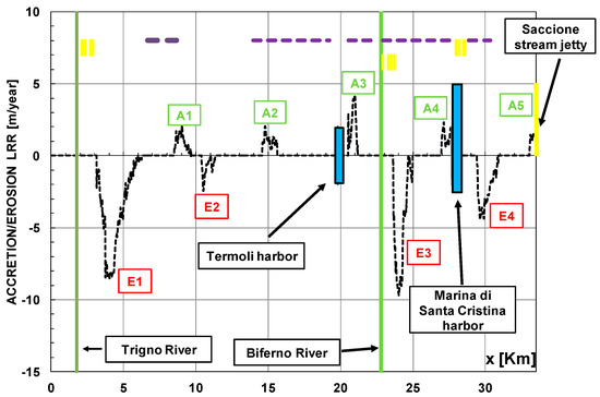
Figure 7.
Erosion/accretion areas LRR function during the period 2004–2016. Horizontal dashes indicate the detached breakwaters; the vertical dashes indicate groin fields.
- The foremost erosion areas (E1 and E3) are located in the southern Trigno and Biferno rivers, with a maximum LRR of −8 m/y and −9 m/y, respectively. In both cases, the retreat occurred just southwards a groin field, which in the case of the Biferno river, is further protected by detached breakwaters;
- The area neighboring the Marina of Santa Cristina harbor has accreted northwards (A4, max LRR +2.2 m/y), and eroded southwards (E4, max LRR −4 m/y); similarly to what was observed above, the erosion zone is located south a groin/breakwater system, which protects the coast for 1.5 km;
- The area just north of the Saccione stream jetty has accreted by nearly 700 m, at a maximum rate of 1.8 m/y.
All the previous outcomes support the idea of a net NW to SE littoral drift.
As indicated in literature e.g., [16,24], the erosion process at the main river mouths (E1 and E3) has been triggered by a reduction in the sediment delivering caused by dam construction. Rosskopf et al. calculated, that in the period 1954–2014, an “average” annual retreat rate occurred in those areas of −2.69 (Trigno River mouth, segment S1 of the Rosskopf et al. paper) and −2.90 (Biferno river mouth, segment S7), respectively.
However, it is noteworthy that despite closing the whole waterfront, shore-parallel barriers at the Biferno river mouth did not stop the erosive trend, although mitigating it appreciably. Table 3 indicates that in this area, the average erosion rate has reduced by 50% compared to the period 1986–1998; in contrast to the neighborhood of the Trigno river mouth (S1, not defended by breakwaters) where the rate of retreat increased by 46%.
Table 3.
Average LRRs at the Trigno and Biferno river mouths.
A dominant NW–SE sediment transport would also explain the origin of the accretion zone A3 (+3 m/y). The latter is located within a “densely structured area”, where a series of detached breakwaters extends for 2 km on the north side of the Biferno river mouth; moreover, a good deal of coast is further defended by rock revetments.
As shown in Figure 8 (lower panel), the accumulation occurred simultaneously to the construction of a new basin of the Termoli harbor; the sediments, made available by dredging operations, were likely conveyed southwards by littoral currents and finally trapped within the structure system. Figure 8 also displays the north shoreline where the detached breakwaters remained substantially stable through the years, with a small accretion area right at the south of the harbor.
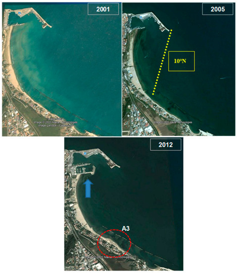
Figure 8.
View of the area A3. Yellow dotted straight line represents sheltering by 10° N waves. (Section 5).
The dynamics from which the areas A2 (+2 m/y), A1 (+1.5 m/y) and E2 (−1.5 m/y) have originated are not readily explained. The accretion areas are located behind long systems of detached breakwaters, which are at a distance from one another of about 5.5 km; however, while A2 is situated at the northern edge of the barriers, A1 is formed at the southern one. Finally, the erosion zone E2 is located nearly 1.5 km southwards of the structures’ end.
To have a deeper insight on these areas, the dominant direction of waves (if any) has to be considered, as well as the variability of shoreline orientation. The effects of both these variables are analyzed in the next sections.
7. The Equivalent Wave Concept and Its Applications
According to Rosskopf et al. [16], a primary need for the comprehension of the Molise coast evolution is establishing more stringent relationships between the wave climate and shoreline response; at this first stage of research, this task is accomplished via the so-called “equivalent wave” (EW) concept, i.e., assuming that shoreline changes may be significantly correlated to a single component of the wave climate.
Although well accepted (and employed) in applied coastal engineering, it is noteworthy that scientists do not agree on the existence of the EW; however, it is surprising to observe how well established this idea might be, even among those researchers who tend to negate it.
Silvester [37] reasoned that “it is normal to correlate volumes of accretion taken over a year with some average swell condition for the same period”, but concluded that “the selection of some meaningful average, including direction, is in the realms of fantasy”. However, the author argued that the annual littoral transport was driven by swells that followed the most intense storms and recognized, in turn, that swells “arrive on a coast from persistent direction”. This implicitly supports the idea that a dominant wave attack for shoreline evolution may exist.
On the other hand, Walton and Dean [38], in examining the directional distribution of littoral drift in many coastal areas, explicitly observed “it was surprisingly similar to that which would occur for a single wave component”. Lately, the authors provided a mathematical explanation of the above finding [39], by adding up a number of sinusoidal components of littoral transport, according to the CERC formula [27].
Anyhow, even assuming such an EW exists, no universally accepted estimation procedure has been proposed to date.
In this study, the EW direction is inferred empirically from the observation of the shoreline trend, and its height and period are estimated via simple averaging operations. Then, several applications are discussed, which are mainly of qualitative nature.
Differently, in the second paper published in this Special Issue [8], the approach of the Littoral Drift Rose is employed [18], and a quantitative comparison is presented for the case of the Trigno river mouth.
Before discussing the results, it is, however, crucial to point out that the whole analysis performed here assumes that a clear shoreline trend exists, at the considered time scale. This was also explained by Hanson and Kraus [25], who argued that the essence of this hypothesis is that waves producing longshore sediment transport and boundary conditions (such as structures) are the main factors controlling the “steady part” of the beach change signal. This “steady signal” is then superimposed by a “noise component” associated with storms, seasonal changes in waves, tidal fluctuations, and other cyclical and random events, such as, potentially, hurricane and typhoon waves, although they are not present at the latitudes investigated here.
7.1. EW Direction and Parameters
According to Pelnard-Considere [40], shoreline orientation at any “un-bypassed” groin is expected to be in every instant nearly normal to the dominant wave attack; hence, it may be taken as an indicator of the EW direction.
For the case under study, of particular interest are the accretion areas A4 and A5 of Figure 7. However, only little information can be drawn from the first, since the beach is protected by detached breakwaters that diffract the incoming waves (Figure 9a).
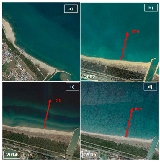
Figure 9.
Panel (a) shoreline neighboring the area A4; panels (b–d), shoreline orientation at the Saccione stream jetty.
Conversely, A5 can freely adjust to the sea and consequently, may represent a more reliable indicator. Panels (b), (c) and (d) of Figure 9 show that this segment of coast has kept a nearly constant orientation in time, which is close to 10° N. Hence, under the hypothesis of straight-parallel bottom contours, the latter can be assumed as the offshore EW direction.
It is noted that 10° N is somehow halfway between the prevailing wave directions indicated by Aucelli et al. [6], i.e., 350° N and 23° N, and corresponds to the angular sector associated with the highest waves in Figure 4. This is consistent with the hypothesis formulated by Silvester [37] that shoreline may be formed by waves correlated to the most intense storms.
Once the EW direction has been established, its height, Hm0E, has been estimated as the average wave height in the directional sector 0–22.5° N (Hm0E = 0.96 m, Figure 3); on the other hand, the peak period, TpE, was simply equal to the mean measured value, 5.08 s.
It is worth noticing that in the applications presented below, the EW characteristics will be assumed constant throughout the coastal area.
7.2. Shoreline Response to Structure Systems
The EW concept has been tentatively used to analyze the shoreline response behind some structure systems. As anticipated, the approach followed here is mainly of qualitative nature and relies on rather crude assumptions; accordingly, the obtained results have to be considered as preliminary.
As a first point, it could be argued that under a 10° N wave attack, the head of the Termoli harbor breakwater completely shelters the shoreline south of it (upper-right panel of Figure 8), and this would explain the aforementioned stability of that reach of coast; then, the resulting diffraction currents, directed northwards, might be responsible for the accretion observed just below the harbor basin. The effect of diffraction is clearly recognizable from the curvature of the shoreline and is consistent with the inversion in the littoral drift direction observed by Rosskopf et al. [16].
Simplified models implemented in GENESIS were employed for the arrays of detached breakwaters neighboring the accretion area A2 and the erosion area E4 in Figure 7. Hereafter, these structure systems will be referred to as SA2 and SE4, respectively. SA2 is located nearly 20 km north the Saccione stream jetty and extends for 2.1 km with an average azimuth of 13° N; the latter, is in fact very close to the EW direction. As shown in Figure 10, the shape of the coast behind the system has remained relatively constant through the years.
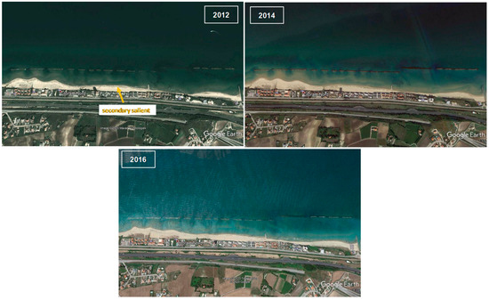
Figure 10.
Shoreline planform at SA2.
The breakwaters have variable length and are either emerged or submerged or “partially underwater”, with alternating submerged and emerged parts; the typical gap width is 30 m. Additionally, two groins are located behind the barriers, the length of which is equal to 50 and 100 m, respectively.
The GENESIS model, pictured in Figure 11a, is made up on a 30 m wide grid, with the initial shoreline parallel to the barrier system; the distance between the structures and the initial shoreline (180–230 m) has been estimated north the breakwaters, from the first null-point of the LRR(x) function. “Pin points” have been used as lateral conditions at the model boundaries, which are located 2 km away from the breakwater ends. The transmission coefficients KT, i.e., the ratio between the wave height right behind the barrier and that just in front of it [3,4,5], have been preliminarily set at 0.4 for emerged barriers and 0.7 for submerged and partially underwater structures. This is basically due to the lack of detailed information on the breakwaters cross section. The equivalent wave has been run for 50 years, to let the beach planform attain a stable shape.
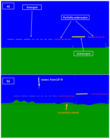
Figure 11.
(a) SA2 as modeled in GENESIS; (b) shoreline response under EW (K1 = 0.1, K2 = 0.15).
In general, simulation results correlate quite well with the observed shoreline trend (Figure 11b; K1 = 0.1, K2 = 0.15); the triple humped salient is reasonably reproduced, although slightly tapered, and so is the coast between the groins.
The shoreline trend behind the first group of barriers is instead somewhat flattened; this is either due to the simplified initial shoreline condition or because GENESIS cannot simulate in detail the multiple diffraction emanating from the short breakwater segments. Moreover, since the partially underwater barrier at the right-end side of the first breakwater group is simulated as a continuous structure, the secondary salient (Figure 10 and Figure 11b) is moved nearly 0.4 Km southwards compared to the observed position.
Interestingly, the simulated average rate of shoreline change around A2 is reasonably like the measured one (Figure 12).
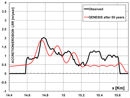
Figure 12.
Observed vs. numerical shoreline change rate at A2.
To check the sensitivity of the solution to the wave direction, the EW angle has been shifted by 10° either to the north or to the south. As shown in Figure 13, waves from 0° N lead to a significant skewness of the main salient, whereas waves from 20° N do not capture the shoreline trend. Obviously, this result does not imply that those waves are ineffective to the shoreline evolution, but rather that their “explanatory power” is smaller compared to that of 10° N.
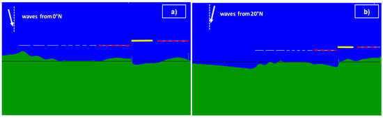
Figure 13.
Shoreline response of SA2 to waves from 0° N (a) and 20° N (b). K1 = 0.1, K2 = 0.15.
As already mentioned, SE4 follows a field of groins located just southwards of the Marina of Santa Cristina harbor. The system, 3 km north the Saccione stream jetty (Figure 14), is made up of two parts. The first includes nine short barrier segments (six emerged and three submerged), whereas the second, 450 m southwards, encompasses four submerged breakwaters. The structures are oriented at 25° N and extend for 1.5 km.
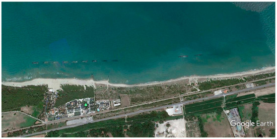
Figure 14.
Shoreline planform at SE4.
The GENESIS model used to study this area has the same characteristics as those described for SA2; however, a 15 m-wide grid was used to better represent either the breakwater segments (30–75 m length) or the gaps (45 m wide). As far as the lateral boundary conditions are concerned, a “gate” has been imposed northwards to simulate the groin system; on the other hand a “pin” point has been set nearly at 0.7 km south to the breakwaters, at the center of a large area where LRR(x) is uniformly zero.
In this case, the EW seems to lead to a shoreline trend that is reasonably consistent with the observations; as shown in Figure 15 (K1 = K2 = 0.1), a wide salient is produced behind the first group of structures, followed by a nearly 1 km-long deficit area corresponding to E4. Furthermore, the latter is again realistically simulated in GENESIS (Figure 16).
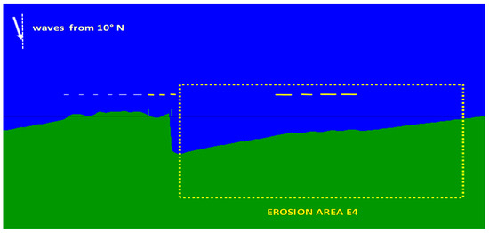
Figure 15.
GENESIS model outputs at SE4 (K1 = K2 = 0.1).
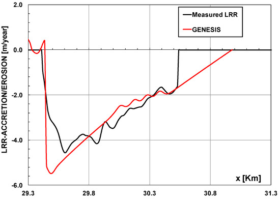
Figure 16.
Measured vs. simulated shoreline change rate at E4.
Figure 17 suggests that a more southern wave attack does not reproduce the shoreline trend properly. However, it stresses that the areas located between the structure groups (breakwater segments or groins) tend to undergo erosion irrespectively of wave direction. For example, the area F1 may erode as “downdrift” effect of either of the breakwater series, depending on whether waves come from the north or the south. The same is valid for the area F2, which is located downdrift from the groin system under wave attacks coming from the north, and downdrift from the first group of breakwaters when the wave climate reverses.
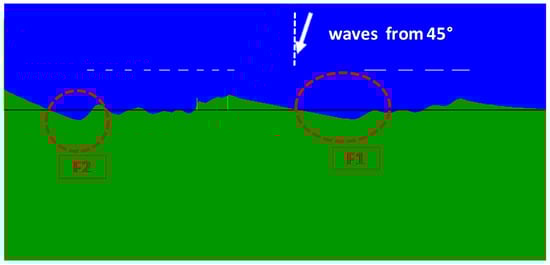
Figure 17.
Shoreline response of SE4 to a 45° N wave attack.
This concept closely resembles the idea of “negative shoreline diffusivity” introduced by Ashton and Murray [41,42] and Walton and Dean [39]. Ashton and Murray showed that when waves break at a straight coast with large angles (more than 40° relative to the normal coastline), the alongshore sediment transport, rather than smoothing the irregularities in the rectilinear trend of the shoreline, may cause the growth of different types of naturally occurring coastal large-scale landforms, including capes, flying spits, and alongshore sand waves. On the other hand, Walton and Dean, extended the Ashton and Murray reasoning and proved that under a bimodal wave climate where most intense wave attacks come from directions significantly inclined (parallel to the shore in the limit), any natural or man-made perturbations tend to continue growing (cusps will accrete and holes erode).
7.3. Features of Recent Coastline Evolution
Besides the shoreline response at relatively restricted areas, the EW may be used to analyze some more general aspects of the recent evolution of the Molise coast.
To this purpose, it is useful to recall that according to a good number of literature studies (see [43]), the rate of littoral drift at a coast segment, Q, can be represented in the following mathematical form:
in which:
- The module Qb depends on both the breaking wave height and sediment characteristics;
- β is the azimuth of the normal coastal segment;
- αb is the azimuth of the breaking wave angle;
For straight parallel bottom contours, Equation (7) can be reformulated in terms of offshore wave parameters, using the conservation of energy and Snell’s law. For the particular case of the CERC formula, it has been shown that (e.g., [18]):
where the subscript “0” denotes deep-water conditions and the module Q0 is a function of both the offshore wave height and period. Hence, assuming Q0 to be constant and the cosine term in the braces nearly equal to 1, from Equation (1) it is readily obtained that:
where x is the alongshore coordinate.
As the first factor on the right hand side of Equation (9) is inherently positive, the sign of the shoreline change (whether accretion or erosion) entirely depends on and . It is, however, worth noticing that as long as Q0 does not vary with x, no structure effect is being taken into account. The cosine term of Equation (9) is shown in Figure 18 for α0 = 10° N. In the same graph, the β angle is also reported, which was obtained after passing the 2004 shoreline measurement through a Godin low-pass filter with a 1 km cut-length; this approach allows keeping the general trend of the coast only, removing any local or structure-induced effects.
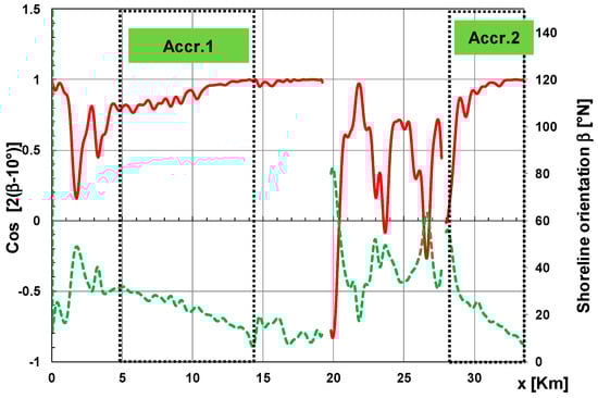
Figure 18.
Cosine term of Equation (9) in red and shoreline orientation (in green).
The Figure shows two potential accretion zones, in which β exhibits a clear decreasing trend and ; the former (Accr.1) extends for nearly 10 km south the Trigno river, whereas the latter (Accr.2) is located between the Marina of Santa Cristina harbor and the Saccione stream jetty. On the other hand, no clear trends have been recognized in the remaining part of the coast.
As displayed in Figure 19, the 2004–2011 LRR(x) function is consistent with the indications in Figure 20; shoreline accretion dominates within the “accretion windows”, apart from the two reaches labelled as “R1”, (corresponding to E1 of Figure 7), and “R2”.
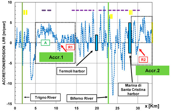
Figure 19.
LRR function during the period 2004–2011.
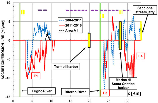
Figure 20.
Erosion/accretion areas for the periods 2004–2011 and 2011–2016.
It is realistic to assume the wide accretion zone “A” to be created at a large extent by the natural orientation of the coast with respect to the incoming waves, with a minor effect due the submerged breakwaters protecting the area. This is basically because its length (about 5 km) is more than twice that of the barriers (2.1 km).
As far as the erosion areas are concerned, R2 is located in the main gap of SE4, and is a well predictable “downdrift” effect of the first group of breakwaters in Figure 15. On contrary, R1 can be hardly considered as a breakwater-induced erosion since it is nearly 1.5 km south of the structures. More likely, this area results from a peculiar orientation of the shoreline or is the effect of the wave climate bimodality not considered in the present approach.
The situation depicted in Figure 19 has dramatically changed during the period 2011–2016. As shown in Figure 20, the erosion area just south the Trigno river has widely enlarged and the retreat created by SE4 has also significantly extended southwards.
In light of this, it can be concluded that the accretion area A1 of Figure 7 (see also Figure 20) represents the tail of a naturally accreting zone, not yet reached by the erosive front propagating from the Trigno river mouth.
This behavior can be reasonably explained as the downdrift effect of the structure systems (groins protecting the Trigno river and SE4) in response to EW; however, the sudden and violent propagation of the shoreline retreat is somewhat surprising and deserves more research.
In this respect, it is noted that such a fast erosion process has occurred in zones where hard protection measures alternate to “free” coastal reaches, which may suggest it could have been enhanced by the aforementioned “negative shoreline diffusivity effect” associated with the wave climate reversal. However, no clear evidence of this is available at the present stage of knowledge.
8. Conclusions
In this paper, a medium-term shoreline change study of the Molise coast has been presented, with the purpose of:
- Highlighting the most recent evolution trends and related shoreline change rates;
- Establishing more stringent relationships between wave climate and shoreline response.
The analysis has been conducted using the LRR as indicator of the coastline evolution; however, a procedure based on the statistical testing of regression results has been adopted, which permits excluding points where the trend is weak or LRR values are influenced by the uncertainties related to data acquisition.
The location and characteristics of the main erosion/accretion areas indicate a dominant NW to SE longshore sediment transport; no hints of possible littoral drift inversion were found.
The present study also confirms the early literature finding that the most intense erosion occurred at the mouth of the main regional rivers Trigno and Biferno. In particular, it has been shown that although the area to the south of the Biferno river is entirely protected by detached breakwaters, shoreline retreat is still continuing at high rates, although the latter are reduced compared to the past.
Section 5 is dedicated to assessing if a dominant wave direction exists (which we call equivalent wave, EW) which could be capable of explaining the main trends of the coastal evolution process. Based on the shoreline development at the Saccione stream jetty, the direction 10° N was selected.
Numerical simulations conducted with the one-line model GENESIS have shown that the use of the “equivalent wave” as a stationary forcing, may lead to a reasonable prediction of shoreline response behind several structure systems, even under crude simplifications of the initial shape of the coast (which has been supposed to be simply straight) and structure characteristics (e.g., uniform transmission coefficient).
Additionally, the EW concept, together with physical reasoning, allowed interpreting the accretion of a significant part of the Molise shoreline between 2004 and 2011.
Finally, in the time interval of 2011–2016, a strong erosive trend was recognized, at both the northern and southern ends of the coast.
Despite that such a strong erosive trend can be reasonably explained as the “downdrift” effect of hard protection measures, the speed at which the erosion areas have propagated southwards is surprising and deserves more research.
In the paper, it is suggested that where rigid structures alternate to undefended shoreline segments, a situation similar to that of “negative shoreline diffusivity” may occur, which could lead to the instability of the shore. This idea, which also applies to the case of the area south from the Biferno river mouth should be accurately verified in future research work.
Author Contributions
M.B.: writing, numerical simulations, data processing, data analysis. G.D.P.: data collecting data processing, data analysis, writing. M.C.C.: numerical simulations, data analysis, writing. G.D.G.: writing and data analysis. C.M.R.: data collecting, data analysis, writing. All authors have read and agreed to the published version of the manuscript.
Funding
This research received no external funding.
Conflicts of Interest
The author declares no conflict of interest.
References
- Dean, R.G.; Chen, R.; Browder, A.E. Full scale monitoring study of a submerged breakwater, Palm Beach, Florida, USA. Coast. Eng. 1997, 29, 291–315. [Google Scholar] [CrossRef]
- Hanson, H.; Kraus, N.C. Shoreline response to a single transmissive detached breakwater. Coast. Eng. Proc. 1990, 22, 2034–2046. [Google Scholar]
- Van der Meer, J.W.; Briganti, R.; Zanuttigh, B.; Wang, B. Wave transmission and reflection at low-crested structures: Design formulae, oblique wave attack and spectral change. Coast. Eng. 2005, 52, 915–929. [Google Scholar] [CrossRef]
- Buccino, M.; Calabrese, M. Conceptual approach for prediction of wave transmission at low-crested breakwaters. J. Waterway Port. Coast. Ocean. Eng. 2007, 133, 213–224. [Google Scholar] [CrossRef]
- Buccino, M.; del Vita, I.; Calabrese, M. Engineering modeling of wave transmission of reef balls. J. Waterway Port. Coast. Ocean Eng. 2014, 140. [Google Scholar] [CrossRef]
- Calabrese, M.; Vicinanza, D.; Buccino, M. 2D Wave setup behind submerged breakwaters. Ocean Eng. 2008, 35, 1015–1028. [Google Scholar] [CrossRef]
- Zanuttigh, B.; Van Der Meer, J.W. Wave reflection from coastal structures in design conditions. Coast. Eng. 2008, 55, 771–779. [Google Scholar] [CrossRef]
- Buccino, M.; D’Anna, M.; Calabrese, M. A study of wave reflection based on the maximum wave momentum flux approach. Coast. Eng. J. 2018, 60, 1–21. [Google Scholar] [CrossRef]
- Bruce, T.; van der Meer, J.W.; Franco, L.; Pearson, J.M. Overtopping performance of different armour units for rubble mound breakwaters. Coast. Eng. 2009, 56, 166–179. [Google Scholar] [CrossRef]
- Van der Meer, J.W.; Allsop, N.W.H.; Bruce, T.; De Rouck, J.; Kortenhaus, A.; Pullen, T.; Schüttrumpf, H.; Troch, P.; Zanuttigh, B. EurOtop, 2018. Manual on Wave Overtopping of Sea Defences and Related Structures. An Overtopping Manual Largely Based on European Research, but for Worldwide Application. 2018. Available online: www.overtopping-manual.com (accessed on 20 October 2018).
- Vicinanza, D.; Caceres, I.; Buccino, M.; Gironella, X.; Calabrese, M. Wave disturbance behind low crested structures: Diffraction and overtopping effects. Coast. Eng. 2009, 56, 1173–1185. [Google Scholar] [CrossRef]
- Buccino, M.; Daliri, M.; Dentale, F.; Di Leo, A.; Calabrese, M. CFD experiments on a low crested sloping top caisson breakwater. Part 1. Nature of loadings and global stability. Ocean. Eng. 2019, 182, 259–282. [Google Scholar] [CrossRef]
- Buccino, M.; Daliri, M.; Dentale, F.; Calabrese, M. CFD experiments on a low crested sloping top caisson breakwater. Part 2. Analysis of plume impact. Ocean. Eng. 2019, 182, 345–357. [Google Scholar] [CrossRef]
- Masria, A.; Iskander, M.; Negm, A. Coastal protection measures, case study (Mediterranean zone, Egypt). J. Coast. Conserv. 2015, 19, 281–294. [Google Scholar] [CrossRef]
- ARPA Emilia Romagna. Studio e Proposte di Intervento per Migliorare L’assetto e La Gestione Dei Litorali di Misano e Riccione; ARPA Emilia Romagna: Bologna, Italy, 2007. (In Italian) [Google Scholar]
- Rosskopf, C.M.; Di Paola, G.; Atkinson, D.E.; Rodriguez, G.; Walker, I.J. Recent shoreline evolution and beach erosion along the central Adriatic coast of Italy: The case of Molise region. J. Coast. Conserv. 2018, 22, 879–895. [Google Scholar] [CrossRef]
- Crowell, M.; Leatherman, S.P.; Buckley, M.K. Shoreline change rate analysis: Long term versus short term data. Shore Beach 1993, 61, 13–20. [Google Scholar]
- Aucelli, P.P.C.; Iannantuono, E.; Rosskopf, C.M. Evoluzione recente e rischio di erosione della costa molisana (Italia meridionale). Ital. J. Geosci. 2009, 128, 759–771. (In Italian) [Google Scholar] [CrossRef]
- Aucelli, P.P.C.; Di Paola, G.; Rizzo, A.; Rosskopf, C.M. Present day and future scenarios of coastal erosion and flooding processes along the Italian Adriatic coast: The case of Molise region. Envrion. Earth Sci. 2018, 77, 371. [Google Scholar] [CrossRef]
- Ciccaglione, M.C.; Buccino, M.; Di Paola, G.; Calabrese, M. Trigno river mouth evolution via littoral drift rose application. Water 2020, submitted. [Google Scholar]
- De Vincenzo, A.; Molino, A.J.; Molino, B.; Scorpio, V. Reservoir rehabilitation: The new methodological approach of economic environmental defence. Int. J. Sediment. Res. 2017, 32, 88–94. [Google Scholar]
- Scorpio, V.; Aucelli, P.P.C.; Giano, S.I.; Pisano, L.; Robustelli, G.; Rosskopf, C.M.; Schiattarella, M. Riber channel adjustments in Southern Italy over the past 150 years and implications for channel recovery. Geomorphology 2015, 251, 77–90. [Google Scholar] [CrossRef]
- De Vincenzo, A.; Covelli, C.; Molino, A.; Pannone, M.; Ciccaglione, M.C.; Molino, B. Longterm management policies of reservoirs: Possible re-use of dredged sediments for coastal nourishment. Water 2019, 11, 15. [Google Scholar] [CrossRef]
- Aucelli, P.P.C.; De Pippo, T.; Iannantuono, E.; Rosskopf, C.M. Caratterizzazione morfologico-dinamica e meteomarina della costa molisana nel settore compreso tra la foce del torrente Sinarca e Campomarino Lido (Italia meridionale). Studi Costieri 2007, 13, 75–92. (In Italian) [Google Scholar]
- Hanson, H.; Kraus, N.C. GENESIS: A Generalized Shoreline Change Numerical Model for Engineering Use. Ph.D. Thesis, University of Lund, Lund, Sweden, 1989. [Google Scholar]
- Hallermeier, W.A. Field data on seaward limit of profile change. J. Waterw. Port. Coast 1985, 111, 598–602. [Google Scholar]
- US Army Corps of Engineers. Shore Protection Manual; Coastal Engineering Research Centre, Government Printing Office: Washington, DC, USA, 1984.
- Hasselmann, K.; Dunckel, M.; Ewing, J.A. Directional wave spectra observed JONSWAP 1973. J. Phys. Oceanogr. 1980, 10, 1264–1280. [Google Scholar] [CrossRef]
- Contini, P.; De Girolamo, P. Impatto morfologico di opere a mare: Casi di studio. In Proceedings of the VIII Conerence Italian Association Offshore and Marina, Forte Santa Teresa, Lerici (la Spezia), Italy, 28–29 May 1998. [Google Scholar]
- Saville, T. The Effect of Fetch Width on Wave Generation; TM-70; US Army Corps of Engineers, Beach Erosion Board: Washington, DC, USA, 1952.
- Hapke, C.J.; Himmelstoss, E.A.; Kratzmann, M.; List, J.H.; Thieler, E.R. National Assessment 528 of Shoreline Change: Historical Shoreline Change along the New England and Mid-Atlantic 529 Coasts; open-file report 2010-1118; U.S. Geological Survey: Reston, VA, USA, 2010; p. 57.
- Edwards Demining, W.; Bridge, R.T. On the statistical theory of errors. Rev. Mod. Phys. 1934, 6, 280–281. [Google Scholar]
- Fan, H. Theory of Errors and Least Square Adjustment; Royal Institute of Technology (KTH): Stockholm, Sweden, 2010; p. 226. [Google Scholar]
- Douglas, B.C.; Crowell, M. Long-term shoreline position prediction and error propagation. J. Coast. Res. 2000, 16, 145–152. [Google Scholar]
- Maiti, S.; Battacharya, A.K. Shoreline change analysis and its application to prediction: A remote sensing and statistics based approach. Mar. Geol. 2009, 257, 11–23. [Google Scholar] [CrossRef]
- Draper, N.R.; Smith, H. Applied Regression Analysis; John Wiley and Sons: Hoboken, NJ, USA, 1985. [Google Scholar]
- Silvester, R. Fluctuation in littoral drift. In Proceedings of the International Conference on Coastal Engineering, Houston, TX, USA, 3–7 September 1984; ASCE: Reston, VA, USA; pp. 1291–1305, Chapter 88. [Google Scholar]
- Walton, T.L.; Dean, R.G. Application of littoral drift roses to coastal engineering problems. In Proceedings of the Conference on Engineering Dynamics in the Surf Zone, Sydney, Australia, 14–17 May 1973; Institution of Engineers: Sydney, VIC, Australia, 1973; pp. 221–227. [Google Scholar]
- Walton, T.L.; Dean, R.G. Longshore sediment transport via littoral drift rose. Ocean. Eng. 2010, 37, 228–235. [Google Scholar] [CrossRef]
- Pelnard-Considere, R. Essai de theorie de l’evolution des forms de rivages en plage de sable et de galets. In 4th Journees de l’Hydralique, les Energies de la Mer.; Question III, Rapport No. 1; Société Hydrotechnique de France: Paris, France, 1956; pp. 289–298. (In French) [Google Scholar]
- Ashton, A.D.; Murray, A.B. High-angle wave instability and emergent shoreline shapes: 1. Modeling of sand waves, flying spits, and capes. J. Geophys. Res. 2006, 111, F04011. [Google Scholar] [CrossRef]
- Ashton, A.D.; Murray, A.B. High-angle wave instability and emergent shoreline shapes: 2. Wave climate analysis and comparisons to nature. J. Geophys. Res. 2006, 111, F04012. [Google Scholar] [CrossRef]
- Van Rijn, L.C. A simple general expression for longshore transport of sand, gravel and shingle. Coast. Eng. 2014, 90, 23–39. [Google Scholar] [CrossRef]


© 2020 by the authors. Licensee MDPI, Basel, Switzerland. This article is an open access article distributed under the terms and conditions of the Creative Commons Attribution (CC BY) license (http://creativecommons.org/licenses/by/4.0/).