Abstract
On the basis of the two-component pressure approach, we developed a numerical model to capture mixed transient flows in close conduit systems. To achieve this goal, an innovative Godunov finite-volume numerical scheme is proposed to suppress the spurious numerical oscillations occurring during rapid pipe pressurization. To dissipate the spurious numerical oscillations, we admit artificial numerical viscosity to the numerical scheme through applying a proposed Harten, Lax, and van Leer (HLL) Riemann solver for calculating the numerical fluxes at the computational cell interfaces. The proposed solver controls the magnitude of the numerical viscosity through adjusting the left and right wave velocities. A wave velocity calculator is proposed to optimally distribute the numerical viscosity over several computational cells around the computational cell in which the pressurization front is located. The proposed solver admits significant artificial numerical viscosity when the pipe pressurization is imminent and automatically reduces it in other places; in this way the numerical diffusion and data smearing is minimized. The validity of the proposed model is justified by the aid of several test cases in which the numerical results are compared with both experimental data and the results obtained from analytical methods. The results reveal that the proposed model succeeds in completely removing the spurious numerical oscillations, even when the pipe acoustic speed is over 1000 m/s. The numerical results also show that the model can successfully capture occurrence of negative pressures during the course of transient flow.
1. Introduction
While responding to a wet flow event, storm water pipe systems experience complex transient flow in which both open channel and pressurized flow regimes may coexist [1]. The resulting transient flows may induce significant positive and negative pressure surges that can be intense enough to compromise the integrity of the system. A 3D multiphase Computational Fluid Dynamic (CFD) model can theoretically replicate the transient flow but it is computationally too expensive and time consuming to be used in the context of the design of such systems that are iterative in nature. Thus, simplified models are usually employed in practice to calculate the transient response of sewer systems in practice. Since mass, momentum, and energy is mainly transferred in the longitudinal direction of the pipe, one-dimensional models have shown to be a reliable tool for capturing the main features of the transient flows in pipe systems.
One of the simplest models employed to calculate transient mixed flow in pipe systems is built upon the rigid water column theory. Wiggert [2], Liou and Hunt [3], and Razak and Karney [4], among others employed the rigid column model both in simple and complex pipe systems and obtained reasonable results. Malekpour and Karney [5] showed that as long as the water column is not locally disturbed, it tends to move along the pipeline as a rigid column. However, more complete dynamic models are required to calculate and trace the waterhammer pressures induced in the system when the flow is locally disturbed in the system.
There are two different types of dynamic models that can be used to calculate transient mixed flow in closed conduit systems [6]. The first one is the shock fitting-based model, which has been widely used in treating transient mixed flow in sewer pipe systems [7,8,9,10,11,12,13,14]. In this method, the interface separating open channel flow from pressurized flow is tracked explicitly by both enforcing mass and momentum conservation across the interface. Having the interface flow characteristics calculated, the flow on either side of the interface is then calculated with its own theory. A variety of shock fitting models have been proposed and shown to provide promising results [7,8,10,15,16]. Nevertheless, interface tracking is the biggest challenge of the shock fitting approach, particularly in complex systems maintaining several simultaneous interfaces. Further, replicating the interaction of the interfaces with themselves and with the boundaries of the system are another challenges of the shock fitting approach; making the implementation of this approach even more difficult.
Shock capturing is another method widely used for calculating transient mixed flows in conduit systems [12,15,17,18,19,20,21,22]. In this approach, both open channel and pressurized flow are treated using a single set of equations governing unsteady flow in open channels. One of the most popular and earliest methods is the Preissmann slot method (generally abbreviated as PSM) [23], named after its innovator engineer Preissmann [24]. In the PSM, a virtual narrow slot above the crowns of the pipe allows the system to remain in an open channel flow condition even when the conduit becomes completely full. The width of the slot is calculated in such a way that the celerity of the wave motion in the slot becomes identical to the pipe acoustic speed; the higher pipe acoustic speed, the narrower slot width. The main drawback of this approach is the spurious numerical oscillation onset when the flow switches from open channel to pressurized flow. Depending on the magnitude of acoustic speed of the conduit, the resulting numerical oscillations could be strong enough to halt the simulation. The second weak point of the Preissmann slot method is that it cannot maintain negative pressures. As soon as negative pressure is about to occur, the flow switches back to open channel flow.
A few novel methods have been proposed to resolve the negative pressure problem. Kerger et al. [19] proposed a negative slot method (NSL) approach in which the mass flow released during depressurization is compensated by a negative slot extended below the crowns of the pipe. In this approach, when negative pressure is imminent, the conduit cross-section is kept full and the mass release required for depressurization of the conduit is compensated from the negative slot; negative depth in the slot measures the magnitude of the negative pressure head. Vasconcelos et al. [25] proposed a two-component pressure approach (TPA) in which the pressure term in the momentum equation is split into two components that measure the flow depth and pressure head in the conduit. Like NSL, when negative pressure tends to occur, the flow depth component is set to the maximum depth of the conduit and the pressure head component is let to calculate the magnitude of the negative pressure. This method has been successfully used for analyzing transient flow in sewer pipe networks [25].
Although experimental results show that both NSM and TPA can calculate both negative and positive pressures quite accurately during the course of the transient flow, they both suffer from spurious numerical oscillations induced when the flow regime changes from open channel to pressurized flow. The intensity of the numerical oscillations depends on the magnitude of acoustic wave speed of the conduit and can be high enough to corrupt the solution. Numerical experiments have shown that beyond an acoustic speed of 30–50 m/s the resulting oscillations tend to corrupt the solution and even cause the computer code to crash. Since the acoustic wave speed in pipes may be significantly higher than 100 m/s, the occurrence of numerical oscillation is a real challenge in the use of PSM and its alternative approaches (NSM and TPA), particularly when the capture of waterhammer pressures is the primary concern of modeling. That is why the cause and remediation of spurious numerical oscillation have been the focus of interest in the last four decades.
In order to suppress the numerical oscillations, researchers have proposed several methods thus far, but most of them have not been entirely satisfactory. Artificially reducing pipe acoustic speed by increasing the slot width is the most popular approach to reduce the numerical oscillation and has been employed by many [15,21,26]. In this method, the numerical oscillations are suppressed through preventing drastic change in wave velocity during flow transition. This approach provides a reasonable model result as long as inertia dominates the flow and the elastic feature of the flow is not of great importance. Otherwise, the magnitude and track of the resulting waterhammer pressures are significantly distorted. Furthermore, in deep and long Combined Sewer Overflow (CSO) tunnels, increasing the width of the slot produces large virtual storage that unrealistically slows down the transient flow discharges and significantly underestimates the filling bore’s speed; this is an issue that is crucially important to the real time operation of pipe systems [5]. An alternative approach is to connect the pipe to the slot by a smooth transition. Sjoberg [27] proposed a transition that smoothly connects the pipe to the slot and employed an implicit finite difference method to solve the equations. The model was shown to succeed in capturing transient pressures free of numerical oscillations. Leon et al. [28] proposed a funnel-shaped slot along with a second-order Godunov-type numerical solution and showed that the model can provide non-oscillatory solutions over a wide range of operational conditions. However, the method is exclusively presented for circular pipes, and it is not applicable for other conduits. Vasconcelos et al. [22] contented that the numerical oscillations have the same root as in a slowly moving shock in gas dynamics (Jin and Liu [29]; Karni and Čanić, [30]; Arora and Roe [31]). They proposed a first-order Roe scheme in which the numerical viscosity of the scheme increases through calculating the numerical fluxes by a so-called hybrid flux method. In the hybrid flux method, the numerical viscosity of the scheme increases by artificially increasing the wave velocities that permit the fluxes to be calculated. The results showed that the hybrid flux method can partially suppress the numerical oscillations, but data smearing becomes significant when the numerical viscosity further increases to completely remove the spurious numerical oscillations. Nonetheless, the test cases presented by Vasconcelos et al. [22] imply that this method can be effectively used only when the pipe acoustic speed does not exceed 100 to 150 m/s. Vasconcelos et al. [22] further proposed a digital filter by which the numerical results obtained in each time step are smoothed before the calculations proceed to the new time step. The results showed that the proposed numerical filter can suppress the numerical oscillations, although like the hybrid flux method, this method is effective only if the pipe acoustic speed is less than around 150 m/s.
Malekpour and Karney [32] proposed a slot method-based model utilizing the Godunov finite volume numerical scheme that employs the Harten, Lax, and van Leer (HLL) Riemann solution for calculating numerical fluxes. To suppress the numerical oscillations, the authors proposed an HLL solver that can automatically add some artificial viscosity to the scheme by increasing the wave velocity in the vicinity of the locations at which the pipe pressurization is imminent. It was shown that this approach can produce oscillation-free solutions even at pipe acoustic speeds of over 1000 m/s.
The dissipative HLL solver proposed by Malekpour and Karney [32] has been successfully employed by other researchers [33,34]. Nevertheless, it is not known if this solver performs well in conjunction with the TPA approach as well because all research thus far has applied the HLL solver in the context of the slot method. Resolving this uncertainty is the main objective of this paper, which will be shown decisively if this HLL solver can also suppress the numerical oscillations while used in the context of the TPA.
2. Theoretical Background: Governing Equations
This conservative form of one-dimensional continuity and momentum equations in open channels can be written as follows [35]:
where, , and are the vectors representing flow variables, fluxes, and source terms, respectively, and can be represented as follows:
where 𝐴 is the flow cross sectional area, Q is the flow discharge, h is the distance between the free surface and the centroid of the flow cross-sectional area, S0 is the bottom slope of the channel, Sf is the slope of energy grade line, g is the gravitational acceleration, ρ is the flow density, R is the flow hydraulic radius, and nm is the Manning coefficient.
As discussed before, regarding PSM, a virtual slot above the crown of the pipe allows pressurized flows to be regulated by the above equation as well. In such a case when the calculated water depth exceeds the pipe diameter, it represents the pressure head in the system, and the amount of mass in the slot replicates the mass compressed in the pipe due to the rise in the pressure head. The width of the slot required to replicate the acoustic wave speed of the pipe (a) can simply be calculated as follows:
where is the pipe cross section, a is pipe acoustic speed, and is the slot width.
In using TPA, it is assumed that the pipe is expanded and contracted during pipe pressurization and depressurization, respectively. In this method, the cross-sectional area of the pipe can be related to the surcharging pressure head () through the following equation (Sanders and Bradford, 2010 [20]):
The above equation accounts for the pipe expansion and contraction due to the pressurization and depressurization phases. It is noteworthy to mention that by multiplying either side of Equation (2) by and performing some algebra, Equation (3) can be easily reached, confirming that both PSM and TPA have an identical underlying concept.
In order to include the effect of negative pressures on the momentum equation, we can rewrite fluxes in Equation (1) as follows:
As can be seen, the pressure term in Equation (1) is split into two terms, and , where measures distance between the free surface and the centroid of the flow cross-sectional area and represents surcharging head. In an open channel flow regime, is set to zero, and when the pipe is pressurized, represents the distance between the crowns of the pipe to the centroid of the pipe cross-sectional area. Note that during pipe depressurization, while the system has sufficient ventilation, negative pressures cannot be maintained. This causes the flow to be switched back to an open channel flow with = 0; otherwise measures negative pressure.
3. Numerical Solution
In this work, the Godunov scheme is utilized to numerically solve the governing equations. The Godunov scheme is an upwind finite volume-based numerical scheme that is widely used for solving partial differential equations [36]. In this method, the spatial domain of the computation is broken down to a number of computational cells with a spatial distance of , and the temporal domain is split by a constant time interval of . The order of accuracy of the Godunov scheme depends on the data reconstruction at the computational cells; piecewise constant data reconstruction provides first-order accuracy and the piecewise linear data reconstruction results in second-order accuracy. In this research, the first-order accuracy is employed because, as will be discussed later, the significant amount of artificial viscosity required for dissipating the spurious numerical oscillations associated with mixed flow modelling prevents the numerical scheme from providing second-order accuracy, even when linear data reconstruction is utilized.
By discretizing Equation (1), unknowns at the current time level can explicitly be calculated on the basis of the data retrieved from the previous timeline using the following equation:
where subscript is the computational cell number; and are upstream and downstream boundaries of the ith computational cell, respectively; is the previous time step; and is the current time step.
Equation (5) can be used to calculate the discharge and flow depth, provided that the flux at the boundaries of the cells are known. In the Godunov scheme, the fluxes at the cell boundaries are calculated through solving the Riemann problem. A Riemann problem includes a system of hyperbolic equations at a flow discontinuity with initial piecewise constant data [36]. The exact Riemann solution can be obtained for the current system of equations, but considering the iterative nature of the solution, it is quite time-consuming, which in turn compromises the efficiency of the numerical analysis. To resolve this problem, approximate Riemann solution can also be utilized to speed up the calculations [36]. Several approximate Riemann solutions have been proposed, including Roe, HLL, and Harten, Lax, and van Leer Contact HLLC [36], among which the HLL Riemann solution is one of the most efficient ones, and thus we utilized it in this study. The HLL Riemann solution was originally proposed by Harten, Lax, and van Leer, who developed it on the basis of the assumption that the generated waves either side of the discontinuity are both of shock wave type. Figure 1 describes the wave structure for the (HLL) solver.
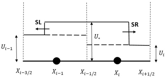
Figure 1.
Wave structure at the Harten, Lax, and van Leer (HLL) solver.
Left and right shock wave velocities can be calculated by the following formula:
In the HLL Riemann solution, if the shock waves move in opposite directions, flux (i.e., at the cell interface can be calculated by cancelling out in Equations (7) and (8). Otherwise, data sampling is required for calculating the fluxes. If the left wave velocity () is greater than zero, the flow would be of a supercritical type and the flux at the cell interface becomes equal to . However, if is less than zero, the flux at the cell interface would be equal to because the flow is supercritical but moves in the opposite direction. The following equations summarize flux at the cell interface under different flow conditions:
Although the first-order Godunov scheme with the HLL Riemann solver generally provides monotonous and oscillation-free solution, it still produces significant spurious oscillations when used in the context of transient mixed flow analysis. Drastic change in wave velocity during the pressurization has been accepted as the key reason of the numerical oscillation. However, more investigation is required to understand under what specific mechanism the change in wave velocity results in numerical oscillation.
Vasconcelos et al. [22] concluded that the post-shock oscillations associated with the PSM have the same origin as slow-moving shocks in gas dynamics [30,31], proposing two different methods for dissipating the numerical oscillations. In the first method, a numerical filter was proposed to smooth the numerical results in each time step. However, this method was shown not to be efficient in higher pipe acoustic speed. In addition, it does not discriminate between spurious numerical oscillation and the numerical oscillations with physical basis. In the second method, a hybrid flux is utilized to gradually add artificial numerical viscosity to the numerical scheme through increasing the wave velocity. This method efficiently suppresses spurious numerical oscillation as long as the pipe acoustic speed does not exceed a certain value (100–150 m/s). Nevertheless, in higher pipe acoustic speed, too much artificial viscosity is required to dissipate the numerical oscillation but at the expense of significant numerical diffusion that compromises the accuracy of the results.
Malekpour and Karney [4] studied the numerical orbits of a first order Godunov numerical scheme with a HLL Riemann solver on the phase plan and realized that artificial numerical viscosity should be admitted only when the flow pressurization is imminent in order to suppress the spurious numerical oscillations. Moreover, they found that adding artificial viscosity only at the computational cell in which flow transition occurs may even exacerbate the spurious numerical oscillations. To resolve this problem, the authors showed that the artificial viscosity should be distributed among several computational cells located around the computational cell receiving flow transition. The numerical results showed that this approach can provide oscillation-free results, even at a high pipe acoustic speed over 1000 m/s. The robustness of the proposed HLL solver by Malekpour and Karney has been confirmed by other researchers [33,34], and thus we adopted it in this research.
In order to show how artificial numerical viscosity can be increased in the HLL solver, consider Equation (9) representing flux at the star zone. Assuming that the absolute value of the left and right wave velocities is equal, we can rewrite flux in the star zone presented in Equation (9) as follows:
The first term on the right-hand side of Equation (10) provides a flux that is unconditionally unstable [37]. This concludes that the second term plays an important role to stabilizing the flux through admitting artificial viscosity to the scheme. This implies that the magnitude of the numerical viscosity can be increased by increasing the wave velocity. It is important to note that adding too much numerical viscosity produces significant data smearing and numerical diffusion, which in turn compromises the accuracy of the results. To control data smearing, Malekpour and Karney [32] proposed a method for calculating the left and right wave velocities that can automatically increase the amount of artificial numerical viscosity in the neighborhood of the pressurization interface. To calculate the wave velocities, we adopted the following formula in this research, which is the adjusted version of that of Leon et al.
where is given by
where is the gravity wave velocity, and the variables with sub-index G are the function of that need to be estimated.
Malekpour and Karney [32] show that if is greater than the height of the conduit, the wave velocity calculated by Equation (11) does not differ from the gravity wave velocity except in the vicinity of the conduit roof. In other words, by using Equation (11), significant artificial velocity is admitted to the numerical scheme only when the water surface in the conduit becomes very close to the conduit roof and the conduit is about to become pressurized. Extensive numerical experiments by Malekpour and Karney produced the following formula for calculating :
where .
By using the above equation, the maximum d is calculated within a number of cells (NS) located on either side the ith cell for which the wave velocity is being calculated. is then calculated by multiplying the maximum d by the factor . In this way, numerical viscosity is distributed within a number of cells rather than being injected just in one cell. If all s are greater than the conduit height, the system is pressurized and a = 1.001 would provide reasonable results. When there is a pressurization front located within the cells, the numerical viscosity is further intensified by applying = 1.4. The number of cells (NS) considered depend on the resolution of the computational grid and should be selected such that the numerical viscosity is adequately distributed on either side of the computational cell for which the wave velocity is being calculated. Malekpour and Karney [32] suggested that the number of cells should cover a distance equal to at least three times as large as the conduit height but in any case it should not be less than three cells. If the ith computational cell is found near a boundary, we should also incorporate the flow depth at the boundary point into Equation (13).
4. Numerical Verification
In this section, the performance of the proposed model is investigated using several test cases. These test cases are to verify different aspects of the model, including (1) the ability of the model in suppressing spurious numerical oscillations induced during the pressurization of conduits under different pipe acoustic wave speeds, (2) the performance of the model in capturing negative pressures, and (3) justifying if the model can capture waterhammer pressures and whether the model adequately discriminates between numerically and physically based numerical oscillations.
4.1. Test Case 1
In this test case, it is shown that the proposed model can efficiently suppress the spurious numerical oscillations without producing significant numerical diffusion. To achieve this, rapid filling is simulated in a horizontal and frictionless box shape conduit with a length of 400 m and with a width and height of 1 m (unit cross-sectional area). The conduit initially maintains a stagnant water column with a depth of 0.6 m when the water level in the upstream water tank is suddenly increased from 0.6 m to 4 m (see Figure 2). Due to its simplicity, this problem has an analytical solution and can be employed to verify the model result. By applying momentum and energy equations, it is easy to show that following the water level rise in the reservoir, a hydraulic bore is set up in the conduit and moves with a velocity of 10.08 m/s [32]. As the bore moves through the conduit, a pressure head of 3.167 m is stabilized in the conduit.
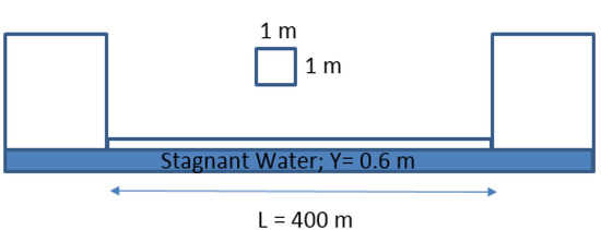
Figure 2.
Schematic of test case 1.
This test case was numerically simulated with a spatial increment of 1 m (400 computational cells) for both the conventional [12] and the proposed HLL Riemann solutions. Figure 3 presents the pressure head along the conduit that was calculated by the conventional HLL Riemann solution at 10 s after the water level rises in the reservoir. The numerical results show that considerable spurious numerical oscillation occurs even when the acoustic speed used is only 50 m/s. The numerical results confirm (not shown here) that by increasing the conduit acoustic speed, the numerical oscillations are violently intensified, eventually resulting in a non-physically sensible solution when the acoustic speed exceeds 300 m/s.
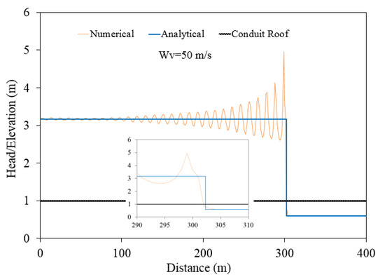
Figure 3.
The numerical results at 10 s after the water level had risen in a test reservoir with an acoustic speed of 50 m/s (conventional HLL solver).
Figure 4 shows the numerical results obtained through applying the proposed HLL Riemann solver with NS set at 5. As can be seen, the model provides oscillation-free solution even at an acoustic speed of 1000 m/s. Nevertheless, some non-significant numerical wiggles with the maximum amplitude of around 1% of the hydraulic depth appear in the result at the Courant number of 0.8. Nonetheless, even this insignificant problem is also resolved when the Courant number i reduced to 0.5. Comparing Figure 3 and Figure 4 reveals that the additional numerical viscosity added by the proposed model does not significantly increase data smearing in the open channel flow section right after the hydraulic bore front.
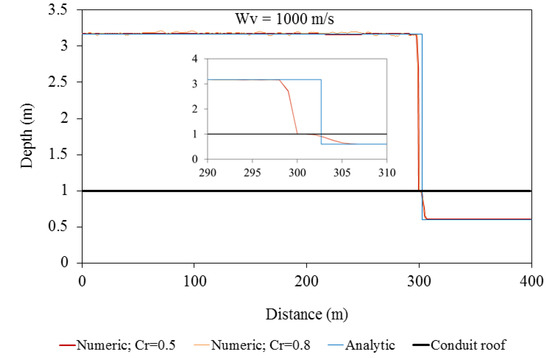
Figure 4.
The numerical results at 10 s after the water level rises in a test reservoir with an acoustic speed of 1000 m/s (proposed HLL solver).
4.2. Test Case 2
This test case make use of the experimental results conducted by Vasconcelos et al. [25]. The performance of the model in capturing both waterhammer pressure and mass oscillation in the system is evaluated. As shown in Figure 5, the test apparatus includes a horizontal acrylic pipe with an internal diameter and a length of 9.4 cm and 14.33 m, respectively, which connects two tanks at its upstream and downstream sides. The upstream tank has a square cross-section with a side and a height of 25 and 31 cm, respectively. The downstream tank, which is a cylinder-shaped tank with an internal diameter of 19 cm, is tall enough to prevent overflow during the experiment. A partially open gate valve at the downstream side of the pipe, in conjunction with an air vent, is utilized to remove air during the filling of the pipe and to induce waterhammer pressure when the filling bore impacts the valve.
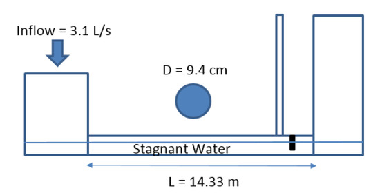
Figure 5.
Schematic of test case 2.
With the pipe initially maintaining a stagnant water column of 7.3 cm, rapid filling was experimented by enforcing a constant flow of 3.1 L/s at the upstream tank. The transient flow in this experiment is dominantly governed by inertia and mass oscillation, but during a short period of time following the contact of the filling bore with the partially open gate valve, the elastic feature of the flow and waterhammer effects become of great importance. Since the pipe and valve head loss coefficients as well as the pipe acoustic speed were not reported in the original work, a calibration procedure is undergone to calculate these parameters. Extensive numerical exploration was conducted with N set to 400, NS of 12, and the Courant number of 0.5 to calculate the best values for the unknown parameters. This procedure ended up with 12, 300 m/s and 0.016 m1/6 for the valve head loss coefficient, acoustic pipe speed, and pipe’s Manning head loss coefficient, respectively. It is worth mentioning that both the acoustic speed and the valve head loss coefficient affect the magnitude of the waterhammer pressure spike and were calculated through an iterative procedure in which these parameters were changed until the calculated pressure spike became comparable to that of the experiment. The Manning coefficient of the conduit affects the pipe filling and mass oscillations inside the downstream tank and thus it was independently calculated.
Figure 6 shows the velocity time-series at 9.9 m from the upstream tank obtained from both the proposed model and the model of Vasconcelos et al. [34]. Both models replicate the experimental data very well, although the proposed model performance is better. The results show that the average discrepancy between the numerical and experimental velocities are around 0.008 m/s. Pressure time history obtained from the proposed model is also compared with the experimental data in Figure 7. As can be seen, the proposed model results are in very good agreement with the experimental data, confirming the validity of the proposed model. Figure 7 also shows that mass oscillation governs the transient flow, except in a very short period of time. The average discrepancy between the numerical and experimental pressure heads is 0.007 m. Waterhammer pressure spike appeared in both experimental and numerical results, is the result of impacting hydraulic filling bore with the partially closed gate. The severity of the waterhammer pressure depends on the magnitude of acoustic wave speed, with the results revealing that an acoustic wave speed of 300 m/s made the numerical results match the experimental results quite well. The calibrated value of the acoustic speed is within the range typically utilized for the pipe material used in the experiment, another confirmation of the validity of the model results.
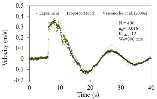
Figure 6.
Comparing numerical and experimental velocity time histories at 9.9 m from the upstream tank.
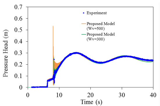
Figure 7.
Comparing numerical and experimental pressure head time histories at 9.9 m from the upstream tank (acoustic speed = 300 m/s).
It is interesting to see that the numerical results obtained from applying an acoustic wave speed of 500 m/s (Figure 7) overestimates the magnitude of the waterhammer pressure but does not affect mass oscillation in the system, which is physically feasible. The magnitude of the waterhammer pressure head rise is two times as high as that produced with an acoustic wave speed of 300 m/s, showing that the model correctly captured the waterhammer effect in the system. Assessing the numerical response in the waterhammer zone reveals that the numerical oscillation remains much longer than what happens in reality. This concludes that the numerical viscosity added by the proposed HLL Riemann solver did not dissipate pressure head oscillation with a valid physical basis.
Finally, the gate valve’s head loss coefficient calculated through the calibration procedure needs to be justified. Assuming a gate discharge coefficient of 0.6, the gate opening associated with the calibrated head loss coefficient of 12 was estimated by the orifice equation as 48%, which seems to be reasonable.
4.3. Test Case 3
In this test case, the experimental study conducted by Vasconcelos et al. [22] is utilized to justify the validity of the proposed non-oscillatory solution during pipe filling. The test rig is similar to the previous test case, with two differences: (1) the pipe has an upslope of 0.1 and (2) there is no gate valve in the pipe (see Figure 8). A stagnant water column causes the initial water depth in the pipe to change from 8.2 cm in the upstream side to 6.7 cm in the downstream side. Rapid filling is implemented through applying a constant flow into the upstream tank. However, since the filling flow rate was not reported in the original work, the upstream boundary condition is treated in a similar way to the approach employed by Leon et al. [16]. Leon et al. assumed that the flow at the upstream tank suddenly increases by 25 cm above the connecting pipe’s bed and remains constant at this level for the rest of the simulation.
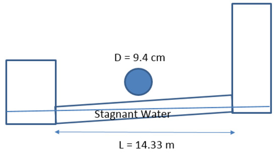
Figure 8.
Schematic of test case 3.
Rapid filling was simulated with the following set of parameters: NS = 12, N = 400 cells, a = 1000 m/s, Cr = 0.5, and nm = 0.011. Figure 9 compares the hydraulic grade lines obtained from the proposed HLL solver and from the hybrid flux approach proposed by Vasconcelos at al. [22] at 6 s from the beginning of the filling. As can be seen in this figure, the proposed approach provides oscillation-free solution at acoustic speed of 1000 m/s but the hybrid flux induces spurious numerical oscillations even at the acoustic speed of 100 m/s. It is worth noting that the numerical diffusion produced by the proposed approach in the open channel flow that occurs right after the filling bore is less than that induced by the hybrid flux method, confirming that the proposed approach admits an optimal amount of numerical viscosity to the numerical scheme. Finally, Figure 9 depicts that the location of the filling bore replicated by the proposed approach at the time of 6 s is around 1 m ahead of that calculated by Vasconcelos et al. [22], implying that the filling bore moved faster in the proposed approach than in that of Vasconcelos et al. To identify the root of the difference, we compared the experimented water level time history in the downstream tank with both the water level time histories obtained from the proposed HLL solver and from the hybrid flux of Vasconcelos et al. As can be seen in Figure 10, the hydraulic bore arrival time to the downstream tank is correctly replicated by the proposed model; this means that the hydraulic bore speed is correctly captured by the proposed model.
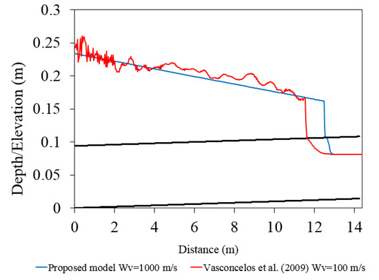
Figure 9.
Hydraulic grade lines at the time of 6 s.
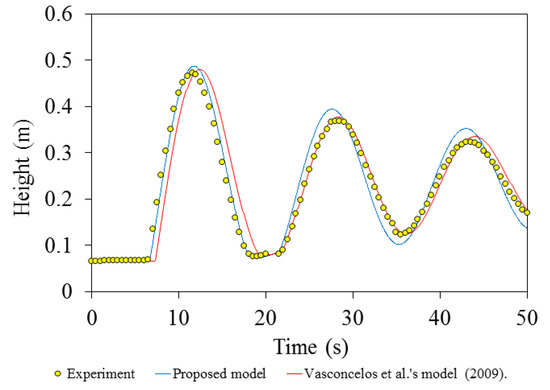
Figure 10.
Water level time histories at the downstream tank.
4.4. Test Case 4
The aim of conducting this test case is to verify that the proposed model can capture negative pressures. We consider a hypothetical frictionless horizontal pipe–reservoir–valve system with a length, pipe diameter, and acoustic speed of 400 m, 1 m, and 1020 m/s, respectively (see Figure 11). The system initially runs at a steady state velocity of 4 m/s when the downstream valve is suddenly closed. This results in a waterhammer pressure spike that runs back and forth without being dissipated as the pipe system is considered frictionless. This test case has an analytic solution that can be utilized as a benchmark for verifying the proposed model’s results. Figure 12 compares the time history of the calculated waterhammer pressure at the downstream end of the pipe with the analytical solution. It can be seen that the model accurately calculates the magnitude and frequency of the induced waterhammer pressures. However, due to the artificial viscosity added to the numerical scheme, some non-physical numerical dissipation occur, that causes the edge of the calculated pressure head time history to be rounded.
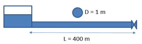
Figure 11.
Test case 4 schematic.
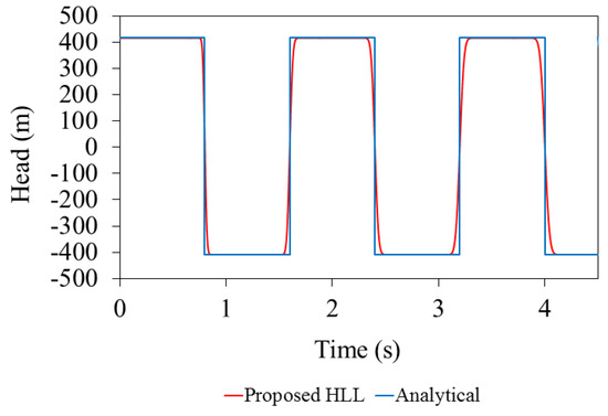
Figure 12.
Waterhammer pressure oscillations.
4.5. Test Case 5
In this test case, the ability of the proposed model in capturing negative pressures is tested through a hypothetical pipe system for which an analytical solution exists. The pipe system consists of two pipes with the profile shown in Figure 13 and an internal diameter of 0.3 m. An upstream reservoir with a constant head of 30 m is utilized to supply the pipe system during filling. A rapid filling is simulated, with the setting parameters being N = 200 cells, NS = 4, a = 500 m/s, and nm = 0.009. The simulation is continued until the whole system is filled, and as shown in Figure 14, the system reaches a steady-state flow condition with a final flow rate of 0.1712 m3/s. Figure 13 compares the calculated steady state hydraulic grade line (HGL) with that obtained from a spreadsheet analysis. As it can be seen in Figure 13, the numerical results coincides with the analytical solution, showing that the model correctly converges to the steady state condition. Obviously, the model also correctly captures the negative pressure occurring within the second half of the pipe.
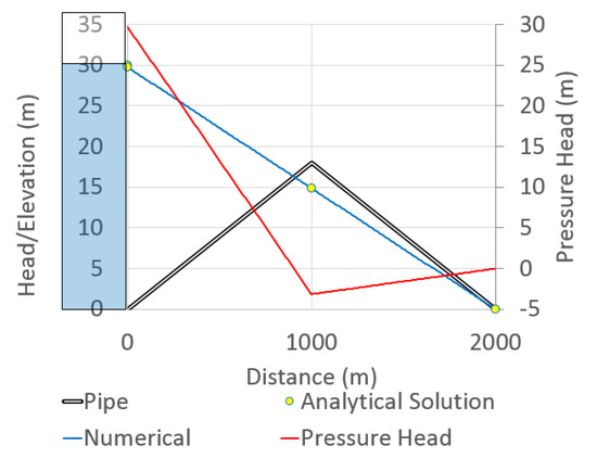
Figure 13.
Established steady state hydraulic grade line (HGL) at the flow rate of 0.1712 m3/s.
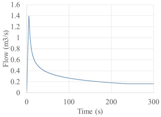
Figure 14.
System flow rate time history.
5. Discussion
Test case 1’s results reveals that spurious numerical oscillations are induced when the flow regime wis changed from open channel to pressurized flow. The numerical oscillations ware attributed to the fact that during the pipe pressurization, the wave velocity drastically increases when the flow is switched from open channel to pressurized flow; the higher the pipe’s acoustic wave speed, the more intensified the numerical oscillations become. In such cases, the conventional Godunov finite volume scheme fails to dissipate the numerical oscillations, with extensive non-physical positive and negative pressure spikes appearing in the solution, which can eventually lead the procedure to the collapse of the computer code. Several studies tended to add artificial velocity only at the computational cell containing the pressurization front, but the results showed that this approach is unable to efficiently dissipate the numerical oscillations, particularly when the acoustic wave speed exceeds 150 m/s. This is far below the realistic pipe’s acoustic wave speed, which may exceed 1000 m/s, depending on the fluid properties, physical characteristics, and rigidity of each pipe. Rather than admitting the artificial viscosity at a local point, the modified HLL Riemann solution utilized in this research distributes artificial numerical viscosity over several computational cells around the cell containing the pressurization front. Test cases 1 and 3 justify that the proposed numerical model can dissipate the spurious numerical oscillations without producing significant data smearing.
To justify that the admitted artificial numerical viscosity does not dissipate the real pressure oscillations with a physical basis, we considered test case 2, which manifested both mass oscillations and waterhammer pressures. As test case 2’s results imply, the proposed numerical scheme discriminates between physical and non-physical numerical oscillations and automatically controls the value of the artificial numerical viscosity without damping the physical pressure oscillations. It is worth mentioning that the artificial numerical viscosity can still affect physical pressure oscillations but the dissipation is too little to compromise the results. Test case 4’s results showed that the model captures severe waterhammer pressure oscillations, and the admitted artificial viscosity also rounds the corner of the waterhammer pressure signals, which is ideally supposed to have rectangular shapes.
Finally, test cases 4 and 5 are used to confirm that the model enables capturing of negative pressures while controlling spurious numerical oscillations. As the results show, negative pressures are correctly replicated by the model but the model is unable to capture water column separation. Test case 5’s results clearly show that the induced negative pressure heads drop to nearly −400 m, but in reality it is limited to the liquid vapor pressure head. As soon as the pressure falls to the vapor pressure head, cavitation forms and the water column is locally separated. Replicating column separation requires more modification to the model, which is currently being perused by the authors.
6. Conclusions
In this paper, we proposed a numerical model to calculate transient mixed flow in close conduit systems. The TPA was utilized to enable the model to capture negative pressures. A first-order Godunov-type finite volume numerical scheme is utilized to numerically solve the governing equations. To dissipate the spurious numerical oscillations, we admit artificial numerical viscosity to the numerical scheme through applying a proposed HLL Riemann solver which is utilized for calculating the numerical fluxes at the computational cell interfaces. The proposed HLL solver controls the magnitude of the numerical viscosity through adjusting the left and right wave velocities. A wave velocity calculator is utilized to optimally distribute the numerical viscosity over several computational cells around the computational cell in which the pressurization front is located. The HLL solver admits significant artificial numerical viscosity when the pipe pressurization is imminent and automatically reduces it in other places; in this way, the numerical diffusion and data smearing are minimized.
Several test cases are presented to justify the validity of the model. The numerical results show that the proposed model completely dissipates the spurious numerical oscillations during flow transition, even at high pipe acoustic speeds over 1000 m/s. The results also imply that the model succeeds in capturing negative pressures during the course of transient flows. This concludes that the TPA with the proposed HLL solver provides a robust and efficient tool for simulating and analyzing transient mixed flow in close conduit systems with a wide range of acoustic wave speeds.
Nevertheless, the proposed model cannot simulate column separation, which may occur when the negative pressure in the system falls close to the vapor pressure of the liquid. Including a column separation feature to the model is something that is being perused rigorously by the authors, and the results will be presented in another paper.
Author Contributions
D.K. conducted the research and prepared the manuscript of the paper, while the Y.H.L. and A.M. reviewed the paper and provided their editorial and technical comments. All authors have read and agreed to the published version of the manuscript.
Funding
This research received no external funding.
Conflicts of Interest
The authors declare no conflict of interest.
References
- Malekpour, A.; Papa, F.; Radulje, D. Uncertainty Analysis in Strom Sewer Collection Systems using Monte Carlo Simulation and Parallel Computing. In Proceedings of the WEAO 2017 Technical Conference, Ottawa, ON, Canada, 2–4 April 2017. [Google Scholar]
- Wiggert, D.C. Transient flow in free-surface, pressurized systems. J. Hydraul. Eng. 1972, 98, 11–27. [Google Scholar]
- Liou, C.P.; Hunt, W.A. Filling of Pipelines with Undulating Elevation Profiles. J. Hydraul. Eng. 1996, 122, 534–539. [Google Scholar] [CrossRef]
- Razak, T.; Karney, B. Filling of branched pipelines with undulating elevation profiles. In Pressure Surges, Proceedings of the 10th International Conference, Edinburgh, UK, 14–16 May 2008; BHR Group: Cranfield, UK, 2008; pp. 473–487. [Google Scholar]
- Malekpour, A.; Karney, B.W. Rapid Filling Analysis of Pipelines with Undulating Profiles by the Method of Characteristics. ISRN Appl. Math. 2011, 2011, 1–16. [Google Scholar] [CrossRef][Green Version]
- Bousso, S.; Daynou, M.; Fuamba, M. Numerical Modeling of Mixed Flows in Storm Water Systems: Critical Review of Literature. J. Hydraul. Eng. 2013, 139, 385–396. [Google Scholar] [CrossRef]
- Bourdarias, C.; Gerbi, S. A finite volume scheme for a model coupling free surface and pressurized flows in pipes. J. Comput. Appl. Math. 2007, 209, 109–131. [Google Scholar] [CrossRef]
- Cardle, J.A.; Song, C.S. Mathematical modelling of unsteady flow in storm sewers. Int. J. Eng. Fluid Mech. 1988, 1, 495–518. [Google Scholar]
- De Marchis, M.; Fontanazza, C.M.; Freni, G.; La Loggia, G.; Napoli, E.; Notaro, V. A model of the filling process of an intermittent distribution network. Urban Water J. 2010, 7, 321–333. [Google Scholar] [CrossRef]
- Fuamba, M. Contribution on transient flow modelling in storm sewers. J. Hydraul. Res. 2002, 40, 685–693. [Google Scholar] [CrossRef]
- Guo, Q.; Song, C.C.S. Surging in Urban Storm Drainage Systems. J. Hydraul. Eng. 1990, 116, 1523–1537. [Google Scholar] [CrossRef]
- Leon, A.S.; Ghidaoui, M.S.; Schmidt, A.R.; García, M.H. Application of Godunov-type schemes to transient mixed flows. J. Hydraul. Res. 2009, 47, 147–156. [Google Scholar] [CrossRef]
- Politano, M.; Odgaard, A.J.; Klecan, W. Case Study: Numerical Evaluation of Hydraulic Transients in a Combined Sewer Overflow Tunnel System. J. Hydraul. Eng. 2007, 133, 1103–1110. [Google Scholar] [CrossRef]
- Song, C.C.S.; Cardie, J.A.; Leung, K.S. Transient Mixed-Flow Models for Storm Sewers. J. Hydraul. Eng. 1983, 109, 1487–1504. [Google Scholar] [CrossRef]
- Capart, H.; Sillen, X.; Zech, Y. Numerical and experimental water transients in sewer pipes. J. Hydraul. Res. 1997, 35, 659–672. [Google Scholar] [CrossRef]
- Leon, A.S.; Ghidaoui, M.S.; Schmidt, A.R.; García, M.H. A robust two-equation model for transient-mixed flows. J. Hydraul. Res. 2010, 48, 44–56. [Google Scholar] [CrossRef]
- Garcia-Navarro, P.; Alcrudo, F.; Priestley, A. An implicit method for water flow modelling in channels and pipes. J. Hydraul. Res. 1994, 32, 721–742. [Google Scholar] [CrossRef]
- Ji, Z. General Hydrodynamic Model for Sewer/Channel Network Systems. J. Hydraul. Eng. 1998, 124, 307–315. [Google Scholar] [CrossRef]
- Kerger, F.; Archambeau, P.; Erpicum, S.; Dewals, B.J.; Pirotton, M. An exact Riemann solver and a Godunov scheme for simulating highly transient mixed flows. J. Comput. Appl. Math. 2011, 235, 2030–2040. [Google Scholar] [CrossRef]
- Sanders, B.F.; Bradford, S.F. Network Implementation of the Two-Component Pressure Approach for Transient Flow in Storm Sewers. J. Hydraul. Eng. 2011, 137, 158–172. [Google Scholar] [CrossRef]
- Trajkovic, B.; Ivetic, M.; Calomino, F.; D’Ippolito, A. Investigation of transition from free surface to pressurized flow in a circular pipe. Water Sci. Technol. 1999, 39, 105–112. [Google Scholar] [CrossRef]
- Vasconcelos, J.G.; Wright, S.J.; Roe, P.L. Numerical Oscillations in Pipe-Filling Bore Predictions by Shock-Capturing Models. J. Hydraul. Eng. 2009, 135, 296–305. [Google Scholar] [CrossRef]
- Abbott, M.B.; Minns, A.W. Computational Hydraulics; Routledge: London, UK, 1998. [Google Scholar]
- Cunge, J.A.; Wegner, M. Numerical Integration of Bane de Saint-Venant’s Flow Equations by Means of an Implicit Scheme of Finite Differences. Applications in the Case of Alternately Free and Pressurized Flow in a Tunnel. La Houille Blanche 1964, 1, 33–39. [Google Scholar] [CrossRef]
- Vasconcelos, J.G.; Wright, S.J.; Roe, P.L. Improved Simulation of Flow Regime Transition in Sewers: Two-Component Pressure Approach. J. Hydraul. Eng. 2006, 132, 553–562. [Google Scholar] [CrossRef]
- Rossman, L.A. Storm Water Management Model User’s Manual Version 5.0; U.S. Environmental Protection Agency: Washington, DC, USA, 2004. [Google Scholar]
- Sjöberg, A. Sewer network models dagvl-a and dagvl-diff. In Urban Stormwater Hydraulics and Hydrology; Yen, B.C., Ed.; Water Resource Publications: Littleton, CO, USA, 1982; pp. 127–136. [Google Scholar]
- Leon, A.S.; Ghidaoui, M.S. Discussion of Numerical Oscillations in Pipe-Filling Bore Predictions by Shock-Capturing Models by JG Vasconcelos, SJ Wright, and PL Roe. J. Hydraul. Eng. 2010, 136, 392–393. [Google Scholar] [CrossRef]
- Jin, S.; Liu, J.G. The Effects of Numerical Viscosities. J. Comput. Phys. 1996, 126, 373–389. [Google Scholar] [CrossRef]
- Karni, S.; Čanić, S. Computations of Slowly Moving Shocks. J. Comput. Phys. 1997, 136, 132–139. [Google Scholar] [CrossRef]
- Arora, M.; Roe, P.L. On Postshock Oscillations due to Shock Capturing Schemes in Unsteady Flows. J. Comput. Phys. 1997, 130, 25–40. [Google Scholar] [CrossRef]
- Malekpour, A.; Karney, B.W. Spurious Numerical Oscillations in the Preissmann Slot Method: Origin and Suppression. J. Hydraul. Eng. 2016, 142, 04015060. [Google Scholar] [CrossRef]
- An, H.; Lee, S.; Noh, S.J.; Kim, Y.; Noh, J. Hybrid Numerical Scheme of Preissmann Slot Model for Transient Mixed Flows. Water 2018, 10, 899. [Google Scholar] [CrossRef]
- Mao, Z.; Guan, G.; Yang, Z. Suppress Numerical Oscillations in Transient Mixed Flow Simulations with a Modified HLL Solver. Water 2020, 12, 1245. [Google Scholar] [CrossRef]
- Chaudhry, M.H. Open Channel Flow; Prentice Hall: Upper Saddle Hall, NJ, USA, 1999. [Google Scholar]
- Toro, E.F. Shock-Capturing Methods for Free-Surface Shallow Flows; John Wiley and Sons: Hoboken, NJ, USA, 2001. [Google Scholar]
- LeVeque, R. Finite Volume Methods for Hyperbolic Problems; Cambridge University Press: Cambridge, UK, 2002. [Google Scholar]


Publisher’s Note: MDPI stays neutral with regard to jurisdictional claims in published maps and institutional affiliations. |
© 2020 by the authors. Licensee MDPI, Basel, Switzerland. This article is an open access article distributed under the terms and conditions of the Creative Commons Attribution (CC BY) license (http://creativecommons.org/licenses/by/4.0/).