1. Introduction
Water is a natural renewable resource dramatically affected by human activity; therefore, its usage must be carefully controlled. Since freshwater represents only 2.7% of the global sources of water, this natural resource around the world is limited. Therefore, its efficient use is one of the greatest challenges of contemporary society [
1]. The scientific research confirms that global warming is a direct result of human activities, causing the change in global atmosphere composition, which is added to natural climate variability [
2]. However, hydrological variability cannot be viewed solely as a result of climate change since it is influenced by so many more factors: heterogeneity of watershed properties, changes in the channel network geometry, river bed geometry alterations, and changes in land-use [
3,
4].
Climate change is reflected in the gradual change in statistical meteorological models valid for a certain region for a period of at least 30 years. Thus, from one year to another, the weather is contrasting [
5]. Climate change leads to the increase in the average temperature with significant variations at regional level, diminishing the water resources used by human populations, reducing the volume of ice caps and thus, raising the sea level, changing the hydrological cycle, increasing the frequency and the intensity of extreme weather events (excessive heat, droughts, floods), etc. [
6]. Regarding the air temperature at the European level, the Intergovernmental Panel on Climate Change (IPCC) remarked an approximately 1 °C increase. The forecast for the next one hundred years is an increase in air temperature up to 6.3 °C in Europe, 5.5 °C for Romania [
7,
8]. In addition, according to data published by the European Environment Agency [
9], water resources for the people of south and southeastern Europe will diminish in the coming years. Although Romania is situated in southeastern Europe, characterized by a temperate climate, and its climate change follows the global warming trend, some particularities appear due to the Carpathian Mountains [
10]. In terms of rainfall, the forecast shows a decrease in precipitation quantities for the summer period with a maximum in July (91%). Furthermore, the annual maximum precipitation will be registered once in March and once around November [
7,
10].
Climate change influences aquatic ecosystems through the action of two main factors: temperature and precipitation (
Figure 1). Thus, the impact of these factors on the surface water quality is practically manifested by drought or floods [
11]. Moreover, the changes in water quality are determined by water temperature increase, which affects the biogeochemical processes operation rate [
12]. Some of these effects are the change in flow volumes, which alter residence time and dilution, increased atmospheric CO
2 concentration, which affects its dissolution rate in water, and finally, changed chemical inputs to the catchments, which disturb the streams’ water chemistry. In the case of lakes and reservoirs, all these processes lead to changes in the trophic state.
Eutrophication was recognized as a pollution problem in European and North American lakes and reservoirs in the mid-20th century, being one of the most serious problems that affect water quality nowadays [
13,
14]. The eutrophication process generally refers to the loading of nutrients to lakes and reservoirs at rates high enough to increase the potential of biological production, decrease water volume, and deplete dissolved oxygen (DO) [
15]. Human activities can accelerate the rate at which nutrients enter ecosystems by the release in the watershed from agricultural or urban sources [
16]. The main effects of eutrophication consist of an increase in turbidity, changes in color, smell, and taste of water, dissolved oxygen depletion, and a phytoplankton biomass increase [
17]. Furthermore, stimulation of the primary production can generate ecological effects such as biodiversity decrease, changes in species composition and dominance, and toxicity effects [
18,
19].
The intensity of the eutrophication process is directly correlated with the aquatic ecosystem hydrodynamics [
20]. Generally, water quality in reservoirs tends to improve due to important outflow, which causes a mixing process with direct consequences on thermocline thickness and depth [
21]. Thus, the trophic state of the lake is improved by reducing the appearance of anaerobic processes in hypolimnion [
22,
23,
24]. Numerous studies have investigated the relationship between reservoir trophic status, water quality, nutrients load, hydrological variability, and so on [
12,
19,
25].
In Romania, the National Administration “Apele Romane” (ANAR) is the national authority in charge of water management and the only one that classifies the water bodies from the water quality point of view. This study aims to verify if the ANAR classification of the Stanca–Costesti reservoir as an oligotrophic lake is still valid, when the Carlson index is used. The classification of water bodies made by ANAR is according to Regulation 161/2006,
Table 1 [
26].
The most sensitive issue related to this classification is that it is done using yearly data, and thus, it is difficult to assess water quality if some indices classify water as being in a certain trophic status, whereas others do in another one.
The Carlson trophic state index is the most well-known and still used, even if there are numerous other classification schemes available [
27].
To assess the trophic state of the reservoir, based on available data (biochemical, inflow, and reservoir water level), the trophic state indices (α) values have been computed. Based on the monthly values of the reservoir water level and inflows for the period 2010 to 2017, data were classified into three groups, namely: wet year, normal year, and dry year and the influences generated by the hydrologic variability (flow and temperature changes) on the trophic state of the lake were investigated.
2. Materials and Methods
Most of the Romanian hydrological network is collected by the Danube river and flows into the Black Sea, apart from some small rivers which flow directly into the sea. The most important water resources in Romania are the surface waters, which consist of inland rivers and the Danube river, bordering the southern part of the country, and both resources are vulnerable to climate variability. To optimize water supplies around the country, more than 1900 reservoirs were created. These ecosystems are quantitatively and qualitatively dependent on direct human influences, as well as on variations of the climate.
Related to the quality of the large lakes and reservoirs in Romania, in terms of trophic state degree, the monitoring of 94 reservoirs regarding nutrient concentrations reveals that 61.7% have a good ecological status/potential, while 38.3% do not meet the required quality objective [
28], mostly due to eutrophication. Romania’s target is to achieve a good status for all surface water and groundwater and good ecological potential for heavily modified water bodies until 2027.
In Romania, there are still major issues regarding compliances with EU regulations, and several hotspots have been identified: lower Danube, the river basins of Arges–Vedea and Buzau–Ialomita, and the north of the Prut–Barlad basin (border with Moldova) [
29]. Prut river basin is located in the northeastern part of the Danube basin, and it is bordered by three major basins, i.e., the Tisa to the northwest, the Siret to the west, and the Dnestr to the northeast, occupying the eastern part of Romania. The Stanca–Costesti reservoir lies on the middle course of Prut River and collects tributaries from Romania, Ukraine, and the Republic of Moldova.
This paper analyzes the effects of hydrologic variability on the Stanca–Costesti reservoir, which, in terms of water volume and covered area, is the second-largest reservoir in Romania and the first in the Republic of Moldova. It was created after the completion of a dam built on the Prut River during 1972–1975, and now it is a border crossing point between the two countries.
Prut river has its source in the Ukrainian Carpathians and flows into the Danube, crossing the Moldavian Plateau and the Romanian Plain. It has 248 tributaries, and its hydrographic basin is elongated, with an average width of approximately 30 km. It is the second-longest river in Romania, having a length of 952.9 km in Romania and 711 km in the Republic of Moldova. The catchment area is relatively symmetrical and is 27,820 km
2, and 10,990 km
2 (40%) is on the Romanian territory [
30]. The drainage network has a length of 11,000 km (33% corresponding to permanent streams while the rest of 67% are due to intermittent streams with temporary discharge), which leads to a density of the drainage network of 0.41 km/km
2, higher than the average value for the Romanian territory (0.33 km/km
2). In terms of land use, 21.4% of the area represents forests, 57% arable land, 1.19% water surface, 13.3% perennial crops [
31].
The Stanca–Costesti reservoir has a watershed of approximately 12,000 km2 (located on the territory of Romania, the Republic of Moldova, and Ukraine), a volume of 1400 million m3, a maximum depth of 43 m, a length of 90 km, covering an area of 590 km2 and mean inflow of 81 m3/s. It has a complex use, allowing the flood attenuation, generation of hydroelectricity at the Stanca–Costesti hydropower plant, water supply for population and industry and irrigation. In addition, it is an integral part of the European ecological network—Natura 2000—in Romania starting in 2004 and in 2007 was declared as a special avifauna protection area.
There are numerous studies presenting the hydrological variability/floods on the Prut River [
32,
33,
34,
35], but the studies regarding the trophic state of this reservoir are scarce. The Stanca–Costesti reservoir is a heavily modified water body, according to National Administration Romanian Waters (ANAR). Its physical characteristics have been substantially changed, and to achieve good surface water status, it is necessary to change its hydromorphological characteristics, which would have a significant adverse impact on the water environment [
28]. The main pressures in the basin are related to insufficiently treated industrial and municipal waters, trespass of water protected zones, accumulation of heavy metals, illegal waste dumping, and inappropriate agricultural practices, which represent up to 65% of the diffuse sources of pollution/emissions in the Romanian part of the reservoir. According to the Danube River Basin District Management Plan, Stanca–Costesti fails the chemical status criterion. Its general physical and chemical conditions are poor, and it does not have a high status for hydromorphology [
36].
In the reservoir area, the climate is tempered with large thermal variations, low rainfall, and long periods of drought. The average annual temperature varies between 7 and 9 °C, the minimum daily temperature being −3.2 °C and the maximum between 38 and 40 °C. The climatic element with an important role in triggering erosion processes is precipitation, whose annual average varies between 500 and 550 mm/year. At the Botosani hydrometric station, a maximum annual value of 964 mm/year was registered in 1912. The distribution of precipitation is represented by approximately 70% rain and 30% snow, with an important quantitative increase in March–June, when 75–90% of the precipitation occurs. Throughout a single year, in the Stanca–Costesti reservoir area, the dominant wind blows from north and northwest direction, with a maximum speed of approximately15 m/s, and the mean speed ranging from 3 to 5 m/s.
Numerous studies reveal that extreme hydrological phenomenon, e.g., drought, flood and flash-flood episodes are very common within the Prut river basin, even during the same year [
32,
33,
34,
35,
37]. Likewise, changes in regional hydrological cycles can be foreseen: earlier snowmelt due to higher air temperature will lead to a different timing of peak streamflow, lower available surface water quantities during summer, increased rainfall variability, and an overall drop in rainfall [
32,
38].
Therefore, it must be mentioned that in the last 15 years, in the Stanca–Costesti area, three catastrophic floods have taken place in 2005, late July 2008, and in September 2010 [
29]. Those events occurred on the Prut River, upstream of the Stanca–Costesti reservoir, generating floods in Romania as well as in the Republic of Moldova, with major damage and even loss of life.
In the aftermath of the same climatic changes, in 2009 and 2012, an increased level of temperature in the warm season was registered.
The country is ranked in the EU just after Poland, the Slovak Republic, and the Czech Republic in terms of floods risks. Annual floods in different parts of the country between 2002–2013 were estimated to have incurred economic losses of more than 6.3 billion euros (the two catastrophic floods in 2005 and 2010 caused more than 100 deaths and total economic losses of 2.4 billion euros). The average annual cost of floods was estimated at 150 million euros for the 2000–2015 period [
29].
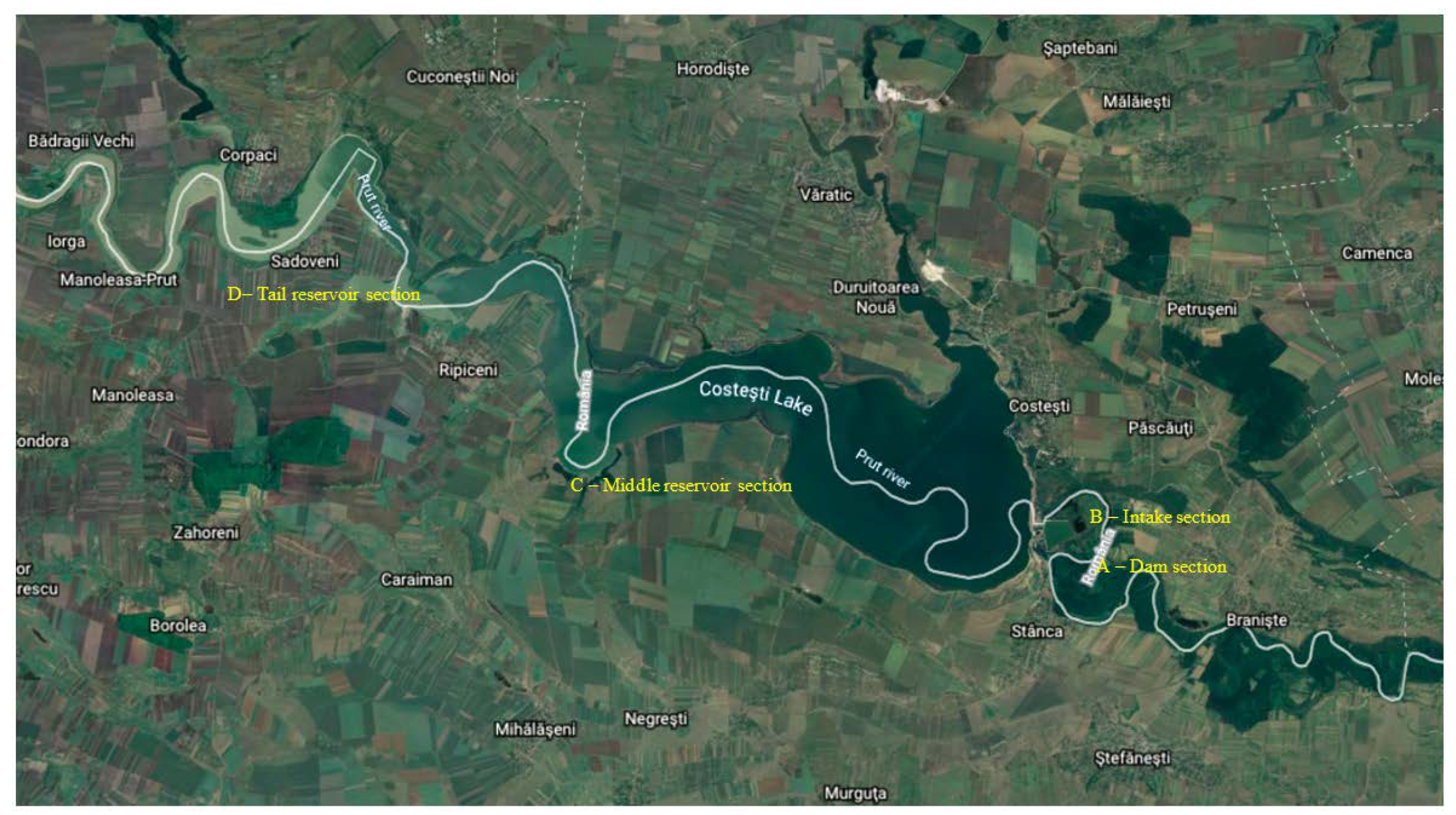
The experimental data used in this research are the integrated samples collected between 2008 and 2017 based on four characteristic points of the reservoir: the dam (A), the intake (B), the middle (C), and the tail (D) (
Figure 2). The frequency of measurement of physicochemical and biological data was according to European norms and was made by ANAR [
39]. To study the hydrochemical regime, the water samples are analyzed during the spring and summer floods and shallow waters in summer and winter. In the upper part of the reservoir, the water samples are taken from the surface (0.2–0.5 m) and in the dam area at three points: 0.2 m and 0.6 m depth and from the bottom.
The evaluation of the trophic state of the reservoirs was made based on the following elements: total phosphorus, total mineral nitrogen, chlorophyll
a, and phytoplankton biomass [
28].
In this study, the actual trophic state of the Stanca–Costesti reservoir was evaluated in relation to the recent severe climatic events in the geographical area of the reservoir, based on experimental data. In the case of the Stanca–Costesti reservoir, it was supposed that the trophic state is given by the biological response to forcing factors, thus using the trophic state indices (TSI).
The ecological status of the lakes and reservoirs is generally assessed according to Carlson’s index. The quantities of nitrogen, phosphorus, and other biologically useful nutrients are the primary determinants of aquatic systems’ TSI. Carlson’s index is one of the most used trophic indices, and it uses the algal biomass as an objective classifier of lakes and reservoirs’ trophic status [
27].
The determination of TSI is based on the algal biomass, nutrients concentrations (phosphorus and nitrogen), and Secchi transparency. TSI provide a way to rate and compare lakes according to their level of biological activity on a range of “0” (corresponding to an ultraoligotrophic lake) to 100 (corresponding to a hypereutrophic lake). A trophic state below 60 indicates lakes with good water quality (oligotrophic through mesotrophic), and values above 60 but below 70 correspond to a highly productive lake with fair water quality (mesotrophic through eutrophic). TSI greater than 70 is for a hypertrophic lake with a poor water quality [
39].
In this study, TSI values were determined by using the following equations:
where:
if TN/TP > 30 then TSINUTRI = TSITP2,
if TN/TP < 10 then TSINUTRI = TSITN2 and
if 10 < TN/TP < 30 then TSINUTRI = (TSITP1+ TSITN1)/2,
with TN, TP, and Chl measured the values of total nitrogen, total phosphorus, and chlorophyll a in the reservoir.
3. Results
According to the hydrological data, the flow with 1% insurance for the Stanca–Costesti reservoir is 2850 m3/s, and the mean inflow for the period 1988–2018 was 79 m3/s, with the highest average monthly inflow in April, 133.6 m3/s, and the lowest one in January, 40.2 m3/s. For the studied period, 2008–2017, the highest average monthly inflow was in July, 155.2 m3/s, and the lowest in November, 38.6 m3/s. This shift regarding the highest value between April and July was determined by the two floods registered in July, in the years 2008 and 2010.
Figure 3 shows the hydrograph of the average monthly flows for the period 2008–2017. The time is expressed in months, where 1st month is January 2008, while month 120 is December 2017.
Figure 4 illustrates, on the same graph, the average monthly flows for each year of the period, and it can be observed that, normally, the maximum inflow corresponded to April.
According to the hydrographs and the variation of the water levels in the reservoir, collected between 2008–2017, the time-lapse of the 10 years targeted were classified into three categories based on the abundance of precipitation: wet years, with average annual flows between 40 and 59 m3/s, 2008 and 2010, years with normal precipitation with average annual flows between 60 and 89 m3/s, 2009 and 2013, and dry years with average annual flows higher than 90 m3/s: 2011, 2012, 2014 to 2017.
However, as compared to the values recorded between 1988–2017, in the last decade, there were considerable deviations from these values, so that for July there was an increase in the multiannual average monthly flow values of about 68%, while for September, a decrease of 46% can be noted. In fact, significant decreases in these values of inflows were observed for the whole period of summer’s end and autumn, whereas in August, there were decreases of approximately 36%, in September of 46%, and in November of 30%.
Figure 5 shows the variation of water levels in the reservoir for the study period; a good correlation with the hydrograph can be observed.
Figure 6 shows the evolution of the water level, inflows, and live storage in the reservoir for the period 2010–2017. In this representation, the flows and levels are represented as a function of time, in which January 2010 is marked with 1 and December 2017 with number 96. There was a good connection between inflows and water level, with a correlation coefficient of 0.6, justified by the major influence of lake entrance flows on the dynamics of the lake.
The physical–chemical indicators analyzed so as to estimate the degree of eutrophication in the Stanca–Costesti reservoir are temperature, dissolved oxygen, nutrients—total nitrogen and phosphorus, and chlorophyll a. The values of these parameters were measured by ANAR.
Changes in the water temperature regime can fundamentally alter water quality. The duration and depth of temperature stratification can also affect the time and volume of water that is isolated during the summer, influencing anoxia and ammonia production and accumulation in the hypolimnion.
Values of the water temperatures recorded for the study period ranged between 0.8 °C (January 2008 and February 2012) and 29 °C (July 2012) [
10], which allowed the consideration that from the thermal point of view, the Stanca–Costesti reservoir fluctuates within the normal variation limits for dimictic lake ecosystems in the temperate areas (
Figure 7).
The evolution of the dissolved oxygen concertation in the Stanca–Costesti reservoir has shown great variations correlated mainly with water temperature evolution (
Figure 7). Thus, the values recorded ranged within a minimum value in August 2015, 2.8 mg/L, and a maximum of 12.7 mg/L in March 2008. Moreover, the evolution of the phytoplankton density in the Stanca–Costesti reservoir recorded a maximum value of 1.77 mil ex./L in September 2009 in the tail of the reservoir section.
For the study period, the total phosphorus concentration recorded values between 0.009 mg/L for the dam section in October 2008 and 0.246 for the middle reservoir section in October 2015 (
Figure 7). This means that most of them were within the permissible limit (0.1 mg/L) for good ecological status.
The quantities of nitrogen, phosphorus, and chlorophyll
a are the primary determinants of aquatic systems trophic state index (TSI). The abundance of nitrogen in the reservoir is justified by the regeneration of this compound in water mass by decomposing organic matter or the contribution of anthropogenic sources. As for nitrogen, it usually decreases during summer due to biological consumption and sedimentation. However, nitrogen concentrations were largely consistent with the average monthly flow of the Prut river. Thus, the greatest values were recorded at the intake and lake’s tail measurement stations, where, at the end of summer in 2016, the value was 2.9 mg/L (
Figure 8).
For the intake measurement section, chlorophyll
a data were not available over the study period. For the rest of the measurement sections, the content of chlorophyll
a determined in the reservoir varied between 0 and 15 μg/L (
Figure 8). The multiannual average monthly values of chlorophyll
a concentration recorded a substantial increase in 2010. Thus, for 2010 the greatest value was recorded in the June–August period due to an extensive algal bloom.
The TSI values for the nutrients and chlorophyll
a obtained for the Stanca–Costesti reservoir (
Figure 9) indicate that the lake is in large proportion in mesotrophic status. Thus, the resulting TSI values for the nutrient concentration shows that the lake was placed in the eutrophic category throughout the period 2008–2017. However, looking at the chlorophyll
a variation, the lake fitted into the oligotrophic stage during 2008 and 2017.
To compute the total TSI, the limiting elements in the lake and the available data were considered. Thus, for the intake section, when calculating the total TSI, the values of chlorophyll
a were not considered. As previously mentioned, for the four measurement sections, there were months with no recordings available for the eutrophication indicators, so that in
Figure 10, there are discontinuities in the computed values.
To allow a more accurate analysis of the total TSI values, these values were represented separately for each measurement section (
Figure 11), which allowed a better classification of the reservoir from the trophic state point of view.
For an easier comparison and correlation of the reservoir’s levels and total TSI values,
Figure 12 presents the TSI values for all four measurement sections. The values are represented according to the number of the day, 1 January 2010 being day number 1, 31 December 2010 is the day 365, and 31 December 2017 is the day number 3612, considering the leap years.
4. Discussion
With regard to the studied period, 2008–2017, in the Stanca–Costesti reservoir, the water temperature varied between 0.5 °C and 29 °C, having the biggest gap for the measurement section (C), middle of the reservoir. The concentration of dissolved oxygen varied between 2.8 mg/L in summer 2015 and 15.5 mg/L in winter 2010. Regarding the time evolution of nutrient content, it was observed that the total mineral nitrogen concentration varied between 0.25 and 2.92 mg/L, while the total phosphorus concentration varied from 0.0035 to 0.025 mg/L. Moreover, the chlorophyll a concentration varied between 0 and 15 mg/L during summer, having maximum values at the measurement section D, tail of the reservoir. A drastic reduction in dissolved oxygen concentration was observed during June–August (between 2.8 mg/L at the intake section and 4.1 mg/L at the tail lake section).
The eutrophication development was analyzed for the Stanca–Costesti reservoir: the evolution of nutrient concentration and biomass in relation to climate change (temperature and precipitation) already recorded in this region. This may be given, on the one hand, by the low diffusion of this element in water and, on the other hand, by higher consumption in the decay processes at the bottom of the lake. It results that the temperature increase as an effect of climate changes may fundamentally alter the habitat of the aquatic organisms and largely depends on internal heat transfer by turbulent and convective processes [
40,
41].
As for the Stanca–Costesti dam, the maximum flow that can be discharged during floods is about 2834 m3/s. From that, 1560 m3/s can be discharged through the surface spillway, 1144 m3/s through the bottom outlet, and 130 m3/s through the turbines of the hydropower plant. During the two floods in the summers of 2008 and 2010, the discharged flow from the Stanca–Costesti reservoir using the three discharge ways simultaneously was up to 2310 m3/s. Because of the two catastrophic floods, the water quality worsened. This is due to the increase in the decomposition process and the organic matter and phosphorus concentrations because of the lake surface layer extension, fueling phytoplankton growth and leading to algal blooms. It was expected that with the important discharge of water, especially by the bottom outlet, the water quality would improve as a direct result of the lake destratification. However, this did not happen, and after the transit of the flood, the dissolved oxygen concentration in the lake decreased to 5.5–7 mg/L, while the phosphorus concentration at the dam section increased up to 0.023 mg/L.
Hydrological variability tends to generate stronger lakes/reservoirs stratification [
42]. This may alter vertical mixing in low-altitude lakes. Lake mixing, however, is especially important to provide oxygen to the deep water and to transport nutrients from the hypolimnion to the epilimnion [
43], preventing nutrient accumulation in the deep water. Furthermore, regular and frequent vertical mixing prevents the build-up of anoxic, reducing conditions in the hypolimnion, which could, in turn, modify the interactions between water and sediments [
42].
Stanca–Costesti is a low-altitude reservoir with multi-annual regulation so that the residence time of water is high. Water stagnation in reservoirs favors the release of nutrients from the sediment layer. Thus, the increase in nutrient loading causes a negative impact on the trophic status of the lake. In the flood periods of 2008 and 2010, the transit of a significant water volume through the bottom outlet of the dam was approved, thereby reducing nutrient loading. This did not happen in 2009, and in March, a substantial increase in nutrient concentration in the lake was observed, especially at the tail (D) and middle (C) reservoir measurement sections. The largest values of nutrient concentration in the lake may be explained by the accumulation of soluble phosphorus and ammonium by the release of nutrients in the hypolimnion layer. These processes depend on thermocline depth, hypolimnetic temperature, microbial decomposition, and oxygen concentration [
44,
45]. In the case of the dam section (A), the situation was better as the outflow of the hydroelectric power plant allowed a local mixing of the water mass. In the following period, the nutrients were strongly assimilated by plants in the epilimnion layer.
According to measured data, it is worth mentioning that during floods, an accentuated increase in total phosphorus appears. Those high values frequently lead to TSI total values greater than 60, which implies a surface water body in an eutrophic state. During floods, the runoff on the surface of the catchment is emphasized, and, as a result, supplementary quantities of phosphorus from agricultural activities are driven. On the other hand, a large amount of water enters the reservoir and intensifies the vertical mixing of water, moving phosphorous from the bottom of the reservoir (hypolimnion) to the epilimnion. Immediately after the flood, an increase in chlorophyll
a concentration is noticed, directly related to the higher quantity of nutrients available in the reservoir [
44,
45].
Pearson’s correlation analysis of water quality parameters was conducted to determine how the eutrophication indicators were correlated with the TSI in the reservoir [
46]. Pearson’s correlation analysis revealed a strong positive and negative relationship between the water quality indicators and total TSI of the Stanca–Costesti reservoir (
Table 2). The correlation between total TSI and TN was positive moderate, with values of Pearson coefficients r = 0.09 ÷ 0.56 with the strongest correlation for the tail reservoir section (r = 0.56). The correlation between total TSI and TP was positive and negative weak/moderate with values in the domain (r = −0.09 ÷ 0.69), with the strongest correlation for the middle reservoir section (r = 0.69). For correlation between the total TSI and Chl, it was not possible to determine r for the intake section due to lack of data, and for the other measuring sections, it resulted in a moderate correlation, negative for the middle reservoir section and positive for the dam and tail reservoir sections. Therefore, we obtained a correlation coefficient between (r = 0.45 ÷ 0.56) with maximum values for the dam and middle sections.
Throughout the entire study period, 2008–2017, Pearson’s correlation coefficients between Chl and TN and TP were weak, around 0.3. For the dam and middle of the reservoir sections, Chl was correlated with TN, while, for the tail of the reservoir section, it was correlated with TP. This shift in the influencing factor, TN or TP, is probably related to different species of algae existing in the measurement sections, the tail of the reservoir being highly influenced by inflows. When considering the different hydrological type of years, Pearson’s correlation coefficient varied from 0.07 to 0.95, as can be seen in
Table 3. Globally, Pearson’s coefficients show a strong correlation during wet years and a weak correlation during dry years. Regarding normal years, the correlation coefficient was strong for the dam and middle reservoir section; however, for the tail of the reservoir section, it was not correlated at all.
As shown in
Figure 9,
Figure 10 and
Figure 11, the total TSI values obtained for the four measurement sections have quite different values. Thus, for the dam, middle, and tail of the reservoir sections, the reservoir can be framed for almost the entire study period in good status (oligotrophic through mid-eutrophic). For the intake section, most of the data frame the reservoir in the poor status (eutrophic through hypertrophic).
Table 4 presents the values of correlation coefficients between total TSI and reservoir water level. It must be specified that for the years 2010 and 2011, experimental data for the dam section were not available. Total TSI values were well correlated with the reservoir water level, the best results being obtained for the dam section. In addition, if we examine the incidence of good correlations for the three types of hydrological years, the best correlations were the values for the dry years 2015 and 2017, and the weakest correlation was for the year 2013, which is considered normal from a hydrological point of view. It must be specified that for the years 2010 and 2011, available experimental data from the dam section were not available.
Apart from the contributions, when considering the lack of data, the limitations of the current study are obvious. However, for assessing the trophic state of any surface water body (including reservoirs), multiparameter indexes, or multicriteria analysis is clearly a better solution. Our study considered only the hydrological variability (e.g., the inflows and water level) and some water quality indicators data. A complete study of eutrophication of surface water bodies requires systematic data to assess all the transformations taking place in the water properly: monthly data related to water quality (physicochemical indicators—temperature, DO, TN, TP, etc. and biological indicators—algal biomass, characteristics, and density, etc.) and catchment characteristics, land use, pollution sources, water uses, hydrodynamic conditions, evaporation, precipitation, atmospheric humidity, etc.
5. Conclusions
The current study aimed to compare the present method used for the characterization of surface water bodies based on Regulation 161/2006, as employed by ANAR, with a method based on the Carlson index. We analyzed rainy periods, with floods on the Prut river, and dry periods, with droughts. Thus, it has been noted how an increased hydrologic variability (as one of the climate change consequences), in terms of floods and droughts, influenced water quality in the Stanca–Costesti reservoir. Due to the prolonged form and geomorphological structure of this catchment, the Prut River is prone to flooding.
According to the results of our study, for the period 2008–2017, the general classification of the Stanca–Costesti reservoir is in the mesotrophic–eutrophic stage. Hence, sometimes, the Stanca–Costesti reservoir experiences changes in the water quality, mainly during the summer periods, and is in the eutrophic state for short periods, with poor water quality and possible negative influences for water usage. The method presented in this study can be applied to any surface water body and provide a better indication of the trophic state than the currently used method in Romania. It is relatively simple to apply based on measurements made by ANAR and can help to adequately manage the use of water considering its trophic status at different times of the year.
Thus, it would be beneficial to consider the possibility of conducting systematic measurements and classifying surface water bodies by using a multiparameter index, such as the Carlson index, or multicriteria analysis, as a more reliable method. In terms of reservoir management, several actions, universally valid, can be implemented to improve water quality in the Stanca–Costesti reservoir: a reduction in nutrient loading entering the reservoir; regular use of the bottom outlet to induce water mixing in the reservoir; active monitoring of water quality and environmental factors; a web platform containing all the monitoring data, used not only by the national authorities and other government agencies involved in water management, agricultural activities, energy sector, and so on but also by researchers and the local community; social awareness actions, to educate citizens and to involve them in the protection of water quality, etc.
Further studies containing detailed temporal analysis on TSI and DO, including correlations between the reservoir water quality and catchment characteristics, land use, etc. must be developed to properly assess the trophic state and the water quality of the Stanca–Costesti reservoir.


