Abstract
The common carp (Cyprinus carpio) is an invasive species in the rivers and waterways of southeastern Australia, and it has been implicated in the serious decline of many native fish species. Over the past 50 years, various control options have been explored, and to date, these have been ineffective or cost-prohibitive. Most recently, cyprinid herpesvirus 3 (CyHV-3) has been proposed as a biocontrol agent because of its high specificity and mortality rate. However, the virus is known to be only effective in a permissive water temperature range of approximately 16–28 °C. To define when this occurs, we undertook a hydrological reconstruction of five diverse river catchments (>130,000 km2) of southeastern Australia over three decades. This confirmed, in the studied areas, that while water temperatures are permissive from spring through to autumn, the time of year that this starts and ends is highly variable, interannually, and with strong latitudinal and altitudinal gradients between and within catchments. The results show that the virus should be effective with respect to water temperature throughout the water temperature range that carp occur in most of southeastern Australia. However, detailed water temperature estimation would still be required to determine the exact week of the start of release in any given catchment. Referring to observations in wild carp populations, we point out the limitation of developing a “release strategy” based solely on water temperature modelling and the need to incorporate fish biology and ecology into this planning.
1. Introduction
Although common carp (Cyprinus carpio, hereafter referred to as carp) was originally introduced in southeastern Australia in the nineteenth century, it was not until the 1970s that it became widespread and by the 1980s it was accepted as a serious invasive species [1]. This recognition followed surveys which showed that, in some parts of the Murray–Darling Basin (MDB), common carp comprised over 90% of the fish biomass with an associated loss of native fish species populations [2]. Nevertheless, carp do not dominate in all hydrological ecosystems in southeastern Australia, and the relative importance of river regulation versus the capacity of carp to be ecosystem engineers, as well as the processes by which they affect water quality are topics of ongoing debate [3,4,5].
Whilst the role of carp as a cause or a consequence of ecosystem decline in the MDB is contentious, less so is the need to suppress the population of carp to achieve native fish recovery [6]. Accordingly, a number of options have been explored over the past 30 years [1], and a National Management Plan was adopted in 2000 [7]. Despite these, no wide-area control has been achieved, with commercial harvest, selective poisoning, genetic control, and physical separation proving either to be ineffective or cost-prohibitive [8].
On the basis of Australia’s success using the Myxoma virus to reduce an invasive rabbit population, spring viremia of carp virus (SVCV) was proposed as a potential biocontrol agent for carp [9]. However, subsequent research has found that the virus was not specific to carp (Fam. Cyprinidae) and even affected non-cyprinid fish such as sheatfish (Siluridae), guppy (Poeciliidae), and northern pike (Esocidae) [10]. Subsequently, viral biocontrol was rejected as an option, and the focus of research became the potential use of sex-biasing genetic modified carp (“daughterless carp”) [11]. Unfortunately, this technology did not fulfil its early promise, at which time viral biocontrol became a more feasible option, due to the detection of cyprinid herpesvirus 3 (CyHV-3) as a cause of mass mortality events in carp in the late 1990s [12]. Subsequently, the virus spread to numerous carp rearing countries, including Indonesia [13], from which an isolate was transferred to Australia’s high quarantine animal health facility, the Australian Animal Health Laboratory (now the “Australian Centre for Disease Preparedness”). Subsequent research confirmed that, unlike SVCV, CyHV-3 was very specific to carp, and did not infect native Australian fish [14].
A feature of many viral infections in fish, including SVCV and CyHV-3, is that infection and disease only occur naturally in a defined water temperature range [15]. For CyHV-3 infection in carp, this range has been established by infection trials to be between 16 and 28 °C [16,17,18]. The existence of a “permissive range” of temperature potentially limits CyHV-3 as a biocontrol agent, particularly if rivers and waterways are only within this range for a short period, or else the water temperature oscillates near the upper or lower threshold, such that infection might not progress to disease. Indeed, a method proposed in aquaculture to immunise carp against CyHV-3 involves infection within the permissive range, and then raising it above this to prevent the appearance of disease [19].
While many factors can influence the complex interaction between the virus and the fish to produce disease, such as CyHV-3 persistence in the natural environment and its capacity for latency [20], water temperature is seen as the most critical driver for a successful virus release strategy. A simple assessment of the potential of CyHV-3 with respect to water temperature has been undertaken using a dataset from a single point beneath a weir in New South Wales, and it has confirmed that the water temperature was within the permissive range for most of the spring, summer, and autumn [21]. However, the generality of this conclusion across the rivers of southeastern Australia is yet to be substantiated, and in particular, whether it applies to intermittently flooded wetlands, which are important for carp’s invasiveness on account of enabling massive recruitment events [22]. Unlike the main river channels, very little systematic water temperature data have been collected, because of the often transient nature of water temperature [23]. Furthermore, because of the complex hydrology of the MDB, it is not possible to simply use air temperature to estimate water temperature, as has been applied in countries with more stable hydrology [24]. Thus, there is a need to integrate air temperature measurements with flow estimates, while also considering the nature of the waterbody [25].
Therefore, the objective of this study was to model water temperature in both rivers and waterways, to a high degree of precision over an extended period. Due to the size of the MDB, we restricted the study to five catchments with a total of 132,129 km2 of drainage area which was representative of the diversity of freshwater environments and the majority of carp habitat found in the basin. A second objective was to assess the extent to which water temperature modelling could be used as the basis for operational planning of the timing of release of the virus, and therefore maximize its activity. For this planning, we reasoned that the ideal would be if the waterbodies entered the permissive range reliably each year at a certain week during the spring warming and remained within it for a period sufficient to readily transmit the virus among the fish. To assess the interannual variability, therefore, we needed to estimate the water temperature over an extended period of time. For further studies, by integrating hydrological and temperature controls into detailed demographic and epidemiological models of carp populations and virus spread, we provided reconstructed hydrological landscapes, incorporating river flow, inundation, and hydrological connectivity together with water temperature. Finally, the results should support the development of a release strategy for CyHV-3 for common carp control in southeastern Australia
2. Materials and Methods
2.1. Selection of Catchments
Carp is predominately in the MDB in southeast Australia, and is mostly absent from Tasmania, Western Australia, and northern tropical Australia [26,27]. They are present, but less abundant in the coastal rivers of southeast Australia [28]. Thus, the target area for the required modelling of the temperature constraints for the release of CyHV-3 is defined to be the MDB and the coastal rivers of southeastern Australia where carp has invaded.
It is not feasible, at this stage, to attempt modelling of the entire MDB, due to its size of 1.06 million km2, or approximately 14% of mainland Australia. To be able to extrapolate results to all southeast Australian rivers based on a subset of catchments, we carefully selected five catchments representing a multitude of landforms and geo-climatic zones. Four of the 23 river valleys and their catchment areas of the MDB and one coastal catchment outside the MDB were chosen (Figure 1). These catchments were selected based on the availability of hydrological data, carp distribution and abundance, including detailed publications on potential control options [8,29]. The selected catchments from north to south were the Moonie River catchment in the north of the MDB and the Lachlan catchment, comprising a relatively colder climate upstream region, undulating hills, irrigated farmland, weirs, dams, and flat riverine plains with interconnected, ephemeral wetlands. Furthermore, we selected two substantive sections of the Murray River, in the mid and lower sections. The two subcatchments with the Murray River in the centre include extensive floodplains and are vital for Australian agriculture. The fifth catchment that was selected was the Glenelg River catchment, a coastal river system within western Victoria. The properties of the five study systems encompassing many of the main landscapes and habitats found throughout the wider MDB [30] are summarised in Table 1. A more detailed description for these catchments is provided in Supplementary Materials S1.
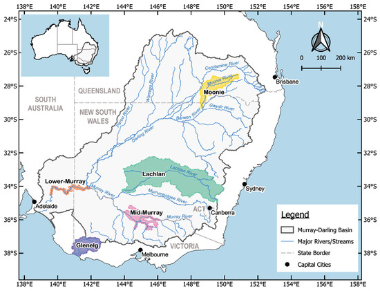
Figure 1.
Catchments in southeastern Australia included in the integrated hydrological study.

Table 1.
Summary of the key hydrological properties of the five studied catchments, data providers, and existing downstream flow modes.
A challenge in undertaking water temperature modelling for CyHV-3 is the complex hydrology of the MDB, with considerable variation in interannual flow and resultant effects on fish biology and recruitment [23]. The underlying driver for this variability is the highly cyclical rainfall pattern over much of the MDB, being driven by El Nino Southern Oscillation (ENSO) cycles [31]. This results in periods of between 2 and 3 years when rainfall is above average, followed by periods of between 3 and 10 years when rainfall is well below average rainfall levels [32]. Thus, in order to inform the water temperature constraints for CyHV-3, as well as the habitat suitability for carp, it was necessary to study the potential impact of variable flow over an extended time period and the connectivity pattern within the catchments. For this, we chose the period from the early 1990s to 2016 for analysis, which included the period of extended drought, the “Millennium Drought” from 2001 to 2009 [33] and the following wet years with high flows in large parts of the country.
2.2. Standardised Methodology for Delineation of Reaches
For the purpose of the current hydrological modelling, as well as the follow-up ecological, demographic, and epidemiological modelling based on hydrological output, it was necessary to define river and stream reaches, which could be presumed to share hydrological properties, such as flow and water temperature. For the rivers and waterbodies of southeastern Australia, there exists relatively mature geographical representations as spatial networks, which are composed of linear segments. Rivers that were of a significant size or where carp survey data existed were incorporated within the network, but minor and non-perennial streams were removed from the dataset.
The river network was extracted from a download of the Australian Hydrological Geospatial Fabric v.3 [34] for the mid-Murray, the lower Murray, and the Moonie Rivers; for the Glenelg River, VicMap Hydro [35] was utilized. The VicMap Hydro network was preferred over the GeoFabric for the Victorian rivers because of its higher spatial resolution (i.e., 1:25,000). For the Lachlan river network, the Geodata Topo 250 K Series 3 Topographic dataset [36] was used.
Physical, man-made structures which would be expected to act as breakpoints, i.e., weirs, bridges, and culverts, were selected from the GeoFabric (or VicMap Hydro) and marked as reach delineators. This list of structures was cross-checked and supplemented by the list of weirs collated by the Murray–Darling Basin Weir Information System [37]. In the case of New South Wales (NSW), a dataset on fish barrier impacts was provided by the NSW Fish Passage Program [38]. This dataset was used as the primary data source for the Lachlan and the NSW region of the mid-Murray catchments as it contained a ranking of the impact the structure posed on fish movement across the barrier.
The spatial network was merged to a multiline string, and a 1 km buffer was applied around these breakpoints to break the network at locations of impact to fish passage. The reach network was also broken at converging or diverging segments, and at river gauge locations so that observed flow data could readily be assigned. Each reach was assigned a unique identifier, and the spatial representation was stored in a PostgreSQL 10.6 (The PostgreSQL Global Development Group)/PostGIS 2.4.3 (The Open Source Geospatial Foundation) database for further connecting hydrologic entities with temperature modelling, as well as usage in a carp habitat suitability and epidemiological model for the selected catchments.
For the waterbodies, we selected all entities that were intersecting a 5 km buffer of the network and where the size was greater than or equal to 2 hectares. For the Moonie and the lower Murray case studies, we used the spatial data derived from the Australian National Aquatic Ecosystem (ANAE) classification for the Murray–Darling Basin [39] and applied a filter based on an attribute for the Water Observations from Space (WOfS) summary statistic [40]. This ensured that we were analysing waterbodies that had an observed water presence of 20% over the WOfS summary period (1987–2014). In the Moonie with often disconnecting reaches, we also integrated 15 waterholes (Jon Marshall, Queensland Department of Environment and Science, personal communication, 2018). In the mid-Murray we applied different WOfS filters, as the major wetland, Barmah-Millewa Forest, had a WOfS value of 1% and the filtered result based on 20% reduced the overall number of modelled waterbodies dramatically. For the Glenelg study, we used the VicMap Hydro water polygons as the spatial entity, as the ANAE dataset only covered the extent of the MDB. Summary figures of the reach delineation for the five catchments are provided in Supplementary Materials S2.
2.3. River Flow
Daily flows, for all reaches in the five selected subcatchments, were estimated for a period from 1990 to 2018 using a combination of observed gauged data and existing models. In cases where the existing observed or modelled data were not sufficient, additional methods, such as interpolation or rational method-based runoff estimations [41] were used.
While two separate hydrological models, integrated quantity and quality model IQQM [42] and eWater Source [43], are available for the Moonie River, these models only provide flows for the main river stem. To estimate flows for the tributaries, we developed a simple rainfall-runoff model based on the rational method and bench-marked the model outputs to the observed flows at the available four gauges and modelled IQQM outputs. The runoff coefficients were estimated based on land use in the catchment.
The surface water flow estimation of the Lachlan River and its tributaries was done based on a combination of flow values derived from the following three sources: (i) Australian Water Resources Assessment (AWRA) output [44], (ii) GR4J hydrologic model [45], and (iii) NSW government’s observed data. The AWRA modelled data are available for 41 stations from 1970 to mid-2014 and were used to patch missing observed data across the catchment. The GR4J model was used to determine stream flows in headwater catchments, where both the AWRA and the observed data were unavailable. Given the availability of observed data at a regular interval across the catchment, the confidence in overall flow estimation was high.
There are close to 200 gauges spread throughout the system on both the main reach and the tributaries of the mid-Murray system, but the majority of these gauges have limited data. Flow data was extracted for the main reach, as well as the tributaries and distributaries, from an eWater Source model [46].
There are ten locks in the lower Murray system which control the hydrology in the system. Daily flow volumes over Locks 1 through 6 are estimated using upstream and downstream water levels and account for the crest level of segments of the weir structure. Daily flow data were exported from South Australia’s hydrological database. Data gaps of less than three days were patched using linear extrapolation. A modified version of the eWater Source Murray Model [46] was used to generate the modelled estimates at lock sites where further data patching was required.
For estimating flows in the main reach of the Glenelg River and its five tributaries, we used flow data downloaded from the Bureau of Meteorology [47]. Missing data were filled in by interpolation. In the case of no gauges in a given sub-reach, data from the closest upstream gauges and any inflows from tributaries were used to estimate the flows. These flows were then cross-checked against the downstream gauges.
Further information on the hydrological regimes and flow modelling in these catchments are available in Supplementary Materials S3.
2.4. Major Storages
There are several large and deep reservoirs with strongly varying water levels included in the selected catchments, for example, the Wyangala and Carcoar reservoirs in the Lachlan, and the Rocklands reservoir in the Glenelg. These storages were separately modelled to derive their seasonal variation in water temperature, including possible stratification. Furthermore, strongly varying water levels in these reservoirs can lead to changes in carp habitat areas. For major storage entities, volume and water level data were available to estimate surface areas. However, no water temperature data were available for these storages, and therefore needed to be modelled.
2.5. Wetland Inundation
Satellite remote sensing was used to determine weekly maximum inundation areas for case study catchments. The MODIS (moderate resolution imaging spectroradiometer) daily time-series images (Terra product “MOD09A” [48]) at 500 m resolution were chosen to model inundation extent from 2000 to 2018. The MODIS inundation model was developed based on the Open Water Likelihood (OWL) index [49]. Taking MODIS daily images clipped to catchment boundaries as inputs, the model delivers weekly maximum inundation extent aggregated from MODIS OWL-detected daily water area within each catchment as output maps. A universal threshold can be applied to automatically delineate inundation extent. Inundation extents in the Murray–Darling Basin detected using MODIS OWL have shown a high degree of accuracy and stability [50,51,52,53,54].
Landsat TM images at 25 m resolution and River Murray Floodplain Inundation Model (RiM-FIM) products [55,56,57] at 5 m resolution were selected to map inundation areas for the time periods prior to February 2000 when MODIS data were unavailable. The advantage of the high spatial resolution of Landsat TM imagery is offset by its low temporal resolution, which can be overcome by the RiM-FIM. The RiM-FIM integrates Landsat TM imagery, Lidar digital elevation model, and flow observations for estimating inundation extent at 1 GL (106 m3) increments in total daily flow ranging from the smallest to the largest recorded flow at a given gauge station [57]. In this study, Landsat inundation mapping was achieved by extracting daily inundating extent either from Landsat TM imagery directly, or from the RiM-FIM products corresponding to an observed daily flow from a selected gauge station in the catchment, and then aggregating daily extent to a weekly maximum area.
Each case study location had various datasets used. Therefore, the inundation modelling varied according to the catchment as follows: For the Moonie, Lachlan, and Glenelg River catchments we used Landsat and MODIS OWL model, whilst for the mid-Murray and lower Murray we used the RiM-FIM model in addition to Landsat and MODIS OWL model. More details of the inundation estimation using the MODIS OWL model and RiM-FIM are given in Supplementary Materials S4.
2.6. Catchment Scale Water Temperature Modelling
2.6.1. Data
Continuous daily water temperature data are only available for a few gauges, and to a large extent monitoring started only in the 2000s. Covering a period from 1990 onward, to simulate carp habitat and virus spread across large-scale river systems, water temperature had to be simulated based on external drivers. For the Murray River and Glenelg, sufficient data are available at a large range of stations, but in the other two catchments data are sparser. For the Murray, we selected only the main stations along the river or on anabranches, usually with long recordings available. For the other catchments, we used all available temperature recordings with at least two years of consecutive data with only minor gaps. However, only a few stations were available with continuous recordings back to 1990 across all catchments. The water temperature station data selected for analysis are listed in Table 2.
Table 2.
Water temperature data used for temperature simulations in the five catchments. The total time span is the sum of all available data for a specific catchment.
Water temperature in rivers and lakes is mainly determined by the heat flux and wind stress across its surface, and heat transported by advection, i.e., flow. Daily meteorological data were sourced from SILO (Scientific Information for Land Owners), a database of historical climate records for Australia given on a 5 by 5 km grid [58]. For each given location, we used the nearest grid point from the SILO database. For lake temperature simulations, we further used wind data retrieved from the Australian near-surface wind speed database available from CSIRO’s Data Access Portal [59]. These data were compiled into gap-free daily data to drive the water temperature models.
We distinguished two modelling approaches, one for rivers and shallow lakes where the vertical heat distribution was usually homogeneous, and the other for deeper reservoirs which stratified seasonally.
2.6.2. Lake Temperature Model
For lakes, there exists a range of one-dimensional, vertical hydrodynamic models to simulate temperature structure over time [60,61]. These are driven by standard meteorological data (irradiance, air temperature, relative humidity, wind speed, and cloudiness) and potentially inflow/outflow time series. Here, we used the one-dimensional k-epsilon turbulence model LAKEoneD [62,63,64] to derive thermal stratification for the three big reservoirs in the Lachlan and Glenelg catchments (Wyangala, Carcoar, and Rocklands reservoirs) and some shallow lakes of the system (Lake Cargelligo and Lake Brewster in the Lachlan catchment). The latter were modelled to be compared with results using the “stream” temperature model and pointed to potential effects of short-term stratification. For the Moonie, the river is often disconnected during times of low or no flow, resulting in a series of waterholes [65]. These waterholes can generate a persistent stratification over short periods of time. This was tested by using the lake model on these waterholes. However, no continuous water temperature was available for these waterholes. We used data for the Brenda Waterhole in the Lower Balonne (Jon Marshall, Queensland Department of Environment and Science, personal communication, 2018), which was in the same climatological region. Water temperature for the Brenda waterhole was measured at a depth of about 50 cm below the surface and a series of loggers further below for the time period from 1 June 2015 to 7 October 2015. Then, the model calibrated to the Brenda waterhole data was used to simulate the daily course of water temperature with a depth resolution of 25 cm for 15 waterholes in the Moonie River catchment, taking into account their hypsometric information and meteorological and wind data, as described above.
2.6.3. Stream Temperature Model
To simulate the water temperature of river reaches, the same principles as for lakes can be applied. Although, for large scale river systems, it is advantageous to use a less complex model. Often, simple correlations between air temperature and water temperature are used. However, these are only applicable for a narrow temperature range. Stream temperature is dependent on the history of air temperature and flow at the location and upstream. This can be used to derive a simpler heat balance without the need to take into account the full heat balance. Here, we simulated water temperature derived from air temperature and flow rates based on the model air2stream [66]. This model parameterises the heat balance using up to 8 parameters or a subset of these [67]. To test this model tool for the five catchments, we applied all possible parameterisations [67], as well as simple regression with air temperature at all locations with available monitoring data (Table 2). The performance of the model was measured by calculating the root mean square error (RMSE) and the Nash–Sutcliffe model efficiency (NSE), where an efficiency of 1 corresponds to a perfect match, 0 indicating that the model performs as well as the mean value of the observation data, and a negative value shows no meaningful simulation.
3. Results
3.1. Reach and Waterbody Delineation
In total, 942 delineated reaches were identified within the catchments varying from 53 reaches within the Glenelg to a total of 502 reaches in the Lachlan (Table 3). The number of reaches was highly correlated with the river length (Pearson’s r = 0.95), and thus the highest number was in the Lachlan (n = 502) and the lowest number was in the Glenelg (n = 53). The lower Murray had a relatively large number of reaches (n = 179) as a result of many regulatory structures along it (n = 31). Reaches ranged in widths from a minimum width of 3 m in the upper Moonie to a maximum width of 176 m in the lower Murray. Overall, average widths per case study ranged from 6.8 m in the Moonie, 13.38 m in the Lachlan, 23.95 m in the Glenelg, and 46.34 m and 77.38 m in the mid-Murray and lower Murray, respectively.
Table 3.
Physical characteristics of the reaches in five case studies.
With respect to the number of waterbodies per catchment, there was a strong correlation with the total waterbody area (Pearson’s r = 0.85), but with several unique features for each catchment. Thus, the mid-Murray has a relatively large number of identified waterbodies, on account of the complex hydrological structure of the Barmah-Millewa Forest, whilst the Moonie has a relatively large number of small waterholes (n = 117).
3.2. Connectivity
Hydrological connectivity within river systems are affected by multiple factors acting across spatial and temporal scales, which themselves interact in complex ways [68]. Distance, climate conditions, or physical-biogeochemical characteristics can play important roles in hydrologic and biological connectivity between wetlands and streams, and between reaches. Hydrologic connectivity was defined as the upstream and downstream reaches having flows greater than 1 ML/day. The reach connectivity in our case studies varied significantly between wet and dry years (Table 4). Especially for those catchments with perennial streams and waterholes, where the Lachlan had a 6% connectivity between reaches in dry years but 83% in wet years, similar for the Moonie with 19.5% versus 43.5% in dry and wet years, respectively. For the mid-Murray, connectivity is nearly always given between reaches while reach to waterbody connectivity is smaller. The lower Murray is well connected between reaches even in dry years and the reach to waterbody connection is relatively high with 78.8% in wet years and 37.4% in dry years.
Table 4.
Percentage of reaches within the catchment where hydrologic connectivity occurred.
For carp movement as well as virus spread the connectivity of wetlands laterally connected to the main river channels plays a dominant role. Due to their shallowness and thus usually homogeneously mixed situation and low to no flow conditions their temperature can be modelled by the river water temperature model using no-flow input, a special case of the general river water temperature model.
3.3. Flow
Estimated flows in the five systems matched the observed flows closely with coefficient of determination (R2) values between 0.80–0.99. Figure 2 shows a comparison between the predicted and observed flows in the mid-Murray system. For the Moonie, flows tend to be lower with higher seasonality as compared with the mid-Murray and lower Murray system.
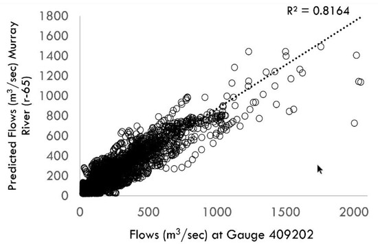
Figure 2.
Validation plot showing flows at the upstream section of the Murray River (reach id 65) and the closest gauge data (Station 409202, Murray River at Tocumwal).
For water temperature modelling, the low flows or even vanishing flows in the northern catchment and, to some extent, in the mid-Murray flow are not a large contributor to temperature variation. This can be different during large flows in the lower Murray or the Glenelg, where heat transport through flow might impact water temperature.
3.4. Water Temperature
3.4.1. Lake Model
Lake thermal stratification simulated with LAKEoneD showed strong stratification for the deep dams. For Lake Wyangala (Lachlan catchment), this led to a permanent low bottom temperature over the year, with a small window of whole-lake mixing, during the winter (Figure 3a). The mean daily air temperature which, on its own, is not a good predictor of surface temperature is overlain in Figure 3a. Comparing results of simulations with the more complex lake model and the stream model driven by only air temperature for shallow Lake Brewster (Lachlan catchment), shows that surface water temperatures are equally well simulated (Figure 3b). Therefore, we used the stream model with no-flow input as the standard water temperature simulation for all shallow water bodies.
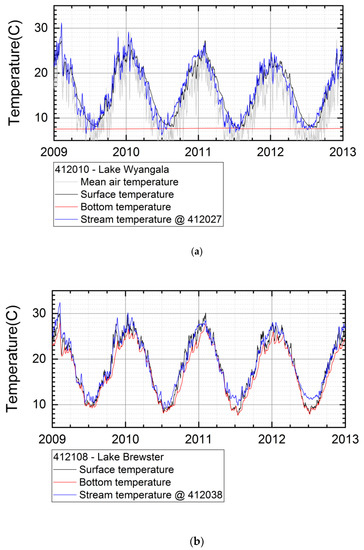
Figure 3.
(a) Deep Lake Wyangala showing strong stratification (low bottom as compared with surface temperature); (b) Shallow Lake Brewster showing week stratification and frequent mixing (similar surface (black) and bottom (red) temperatures) with similar results for lake and stream model (blue). The grey line shows air temperature.
As the deep reservoirs simulated in this study have a relatively cold hypolimnion, the water temperature at the dam outlet can be low, depending on outlet depth and water level. This often leads to downstream cold water pollution [69]. This effect can be seen in the water temperatures downstream of the two large dams in the Lachlan catchment, which are significantly lower than stream temperatures in neighbouring reaches. A more detailed river model, including dam operation, would be needed to model this type of cold water pollution [70]. As the stream model simulates the water temperature based on “learning” from historical data, it will generally generate adequate water temperatures, as long as the dam operation is similar in the simulated years. With the current model, it was not possible to simulate changes in dam operation under strongly fluctuating water levels, or climate change in future conditions affecting downstream stream temperatures in a different way. This effect was limited to a only small number of upstream dams and would not significantly alter habitat and virus spread based on water temperatures as simulated for the five catchments. In river reaches potentially affected by cold water pollution, the virus release strategy must be analysed case by case in close relation with dam operation.
3.4.2. Stream Model
Stream water temperature models with p = 3, 4, 5, 7, and 8 parameters in air2stream [67], as well as a regression with air temperature, were tested. The simulated water temperature is exemplified for the Lachlan River at Cowra (Station 412002). Figure 4 shows the entire simulated period, the annual cycle over a period of four years, and a detailed view of the seasonal cycle for the 2010/2011 year. Air temperature is overlain on the plots for water temperature, and flow rates are shown in a separate plot. The best models are achieved using parameterisations p = 7 and p = 8, which include streamflow as a predictor (Table 5). Models not including streamflow generally are less optimal. However, in cases where there is no flow, models p = 8 and p = 4 generate non-valid temperatures due to a divide by zero operation. Therefore, we generally used model p = 7 depending on the NSE value, as no-flow conditions were common in the region. The simple regression model with air temperature, in all cases, resulted in inferior simulations for water temperature and should be avoided when predicting water temperatures.
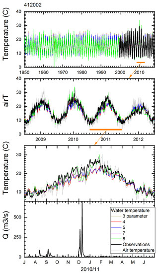
Figure 4.
Observed and simulated stream temperatures using different model parameterisations and flow rate for Station 412002 (Lachlan River at Cowra). Observations (black lines), simulations (coloured lines), air temperature (grey lines). Top panel is the entire simulation period followed by a four-year period and a close view of the seasonal cycle in 2010/2011, with zoom ranges depicted by orange bars and arrow. The bottom panel shows flow rates during this year.
Table 5.
Root mean square error (RMSE) and Nash–Sutcliffe model efficiency of stream model at Station 412002 (model p = 2 is a simple regression model between air and water temperature). Model parameter p according to Piccolroaz et al. [67].
For the specific case of the Moonie River, separating in a series of disconnected waterholes during no-flow conditions, we simulated 15 waterholes using the lake model and compared them with the stream model using only air temperature as the predictor variable. The different waterholes are in the same climate region. Thus, their water temperature is similar, only showing variations based on their different hypsometry (see Supplementary Material S5 for hypsometric data and simulation details). The lake model was calibrated using a small set of continuous data available for the Brenda waterhole in a neighbouring catchment. Figure 5 shows simulation results for surface water for waterhole r78 at Fenton as compared with recorded water temperatures nearby at Station 4170204A (Moonie at Fenton). The simulations of the two different models show good performance with regards to the observations. Thus, also for this partially disconnecting river system, the air2stream water temperature model shows good simulation performance. In general, the NSE for the simulations using air2stream with the seven-parameter model is in the range above 0.85 for all stations in the five catchments.
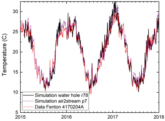
Figure 5.
Comparison between observed water temperature (Station 4170204A at Fenton, Moonie) and simulated water temperatures for this location using the air2stream model with p = 7 parameters [67] (purple), and the LAKEoneD lake temperature model for water hole r78 (black).
The stream model represented measured water temperature very well in all 64 locations with available temperature data for the five catchments. According to the reaches defined for the catchments, then, we selected the closest grid point from the SILO climate database and used mean air temperature for this point to simulate the water temperature in this reach using the closest available water temperature model. For the three large reservoirs in the Lachlan and Glenelg catchment, we used the lake model to derive surface water temperature.
Modelled water temperatures are available for a period from 1990 to 2018 for all 942 reaches to be used in further analysis and as the basis for ecological and epidemiological models together with flow rates and inundation data.
Further background on water temperature modelling results is presented in the Supplementary Materials S5.
3.5. Water Temperature and Permissive Virus Activity
Virus activity is dependent on water temperature. Assuming a permissive range of 16–28 °C, we can show the changes in timing for positive activity in all five simulated catchments. Figure 6 represents the monthly statistics (box plot) for selected reaches in all five catchments, ordered from north to south, superimposed with the band of assumed range of virus permissibility. Windows of opportunities for a virus release are strongly dependent on geoclimatic location. While in the Moonie and the lower regions of the Lachlan, the summer months are potentially too warm with respect to permissive water temperature; the lower Murray and Glenelg River sections show that summer water temperatures are in the optimal range. This also means that the window of opportunity is smaller and broken up in a pre- and post-summer period in the northern catchments, while for the more southern rivers, a single window of opportunity reaching from October/November to March/April is possible. In the case of stream reaches experiencing cold water release from upstream dams (see the Lachlan example in Figure 6b), the whole year is not, or only suboptimal, with respect to virus activity. This implies that dam releases must be done in accordance with a release strategy.
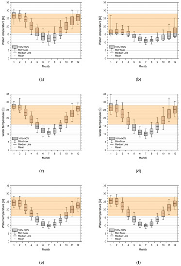
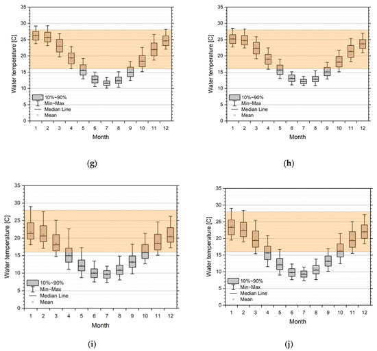
Figure 6.
Monthly statistics of simulated water temperatures from 1990 to 2015/2018 in the five catchments from north to south. Overlay is a suggestive orange band of permissive temperatures (16–28 °C) for virus activity. (a) Moonie station (417204A Fenton). Lachlan stations; (b) Upper river section, station 412067 d/s Lake Wyangala; (c) Mid-river section, station 412038 Willandra; (d) Lower river section, station 412194 4_Mile. Mid-Murray stations; (e) Upper river section, station 409025 Yarrawonga; (f) Lower river section, station 409207 Torrumbarry. Lower Murray stations; (g) Upper river section, station 4260501 Lock 9; (h) Lower river section, station 4260902 Lock 1. Glenelg stations; (i) Upper river section, station 238206 Fulham Bridge; (j) Lower river section, station 238224 Dartmoor.
However, this summary picture of the average seasonal cycle does not show the strong interannual variability, nor does it differentiate the distribution of permissive ranges and non-permissible ranges over several years or clearly show the full north-south gradient in permissibility range. For this, we can concentrate on the number of reaches in each catchment, where the temperature for virus activity is permissible (here 16–28 °C). Figure 7 shows the seasonal variation by plotting all simulated years for each catchment. In the Moonie, the range can be met over most of the year with a small non-permissible period during winter, when temperatures become too cold on average. However, the interannual variability is high during the rest of the year, which is partly due to low flow and disconnection of the stream yielding a reduction in reach numbers falling into the permissible temperature range. While the Moonie shows a very high interannual variability in reaches in the permissible range, the other four catchments show clearer periods of permissible ranges. This being the largest in the lower Murray and Lachlan, while mid-Murray and Glenelg show smaller periods. This can be attributed to more pronounced winter-summer temperature regimes. A detailed analysis of the first and last week, when temperature is in the permissible range, is given in Table 6. On the rising limb of temperature during spring, the permissive range is reached (median value) at week 39 for the lower Murray and at week 46 for the Moonie. In addition to this general difference between catchments, there is also an altitudinal difference. In the southern catchment of the Glenelg, the time when the temperature enters the permissive range is ten weeks behind that of the northern Moonie; for the Lachlan River, the lowland rivers and waterway areas become permissive for virus activity an average of seven weeks before the montane areas. According to Figure 6 and Figure 7, one could set up a general rule for virus release taking into account interannual climate variability, and thus changes in water temperature. To support this further, one can plot the annual cycle of reaches which are below, above, or within the permissible range, and add the information when reaches are likely not connected, i.e., periods with no flow (Figure 8). This clearly shows that, in the Moonie, disconnection, and thus waterholes, is a common phenomenon, in which case a virus release is not recommended, because fish to fish contact, as the main mechanism of virus transmission, is not effective, even when water temperature would allow this. This can happen in reaches of the Lachlan, mid-Murray, and Glenelg as well, but is unlikely for the lower Murray. The latter shows a regular seasonal cycle of permissible range for virus activity with less interannual variation. Water temperatures inhibiting virus activities are not very common in all five catchments during times of free-flowing water.
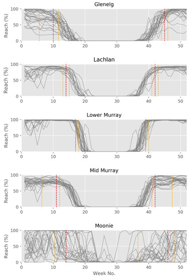
Figure 7.
Annual cycles of the number of reaches within the permissible temperature range for virus activity. Each line represents a single year. Red lines within the winter-summer period indicate the median first week over the entire time series where 80% of reaches are within the optimal permissive range, and during the summer-winter period, the red line represents the last week where 80% of reaches are within the optimal permissive range. Orange lines represent the 20th and 80th percentiles for both spring and summer. For values see Table 6.
Table 6.
Percentile values of the first and last week of the entire time series where 80% of the reaches within a catchment are within the permissible range for virus activity.
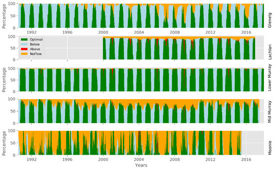
Figure 8.
Percentage of reaches with water temperature in the permissible range of virus activity (green), below (light blue), above (red), and where no flow is present (yellow).
For a virus release, it is necessary that the momentary water temperature is in the permissible range and that the permissible range is sustained over a longer period (weeks) to allow virus transmission. The consecutive number of weeks that water temperature is in the permissible range is shown in Figure 9 as a box plot for each catchment. It clearly shows that the permissible range is reached, on average, in only five weeks in the reaches of the Moonie. It is around 12 weeks in the Lachlan, Glenelg, and the mid-Murray, although all three catchments have significantly different temperature ranges. This shows that water temperature alone is not sufficient to determine the permissible periods for virus release. Here, connectivity also plays an important role. In the well-connected lower Murray, water temperature is the main factor for defining a permissible range of virus activity, seen in a large range of 13 to 29 consecutive weeks, significantly larger than in the other four catchments.
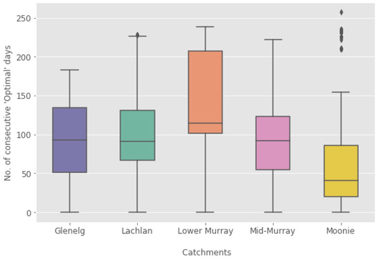
Figure 9.
Summary box plot of the number of consecutive days with water temperature in the permissible range of virus activity.
4. Discussion
Defining constraints for carp herpesvirus release in a large connected river basin needs the interplay of various modelling and computational techniques to be successful. Large scale hydrological models are available for parts of the Australian system, or worldwide. The status of connectivity between water bodies over large regions can only be achieved by using remote sensing technology. Connectivity might be a lesser issue in regions with regular flow characteristics but is an essential part of flood inundation and disease spread modelling in slow-flowing, lowland river systems. The high variability of climate conditions in Australia, which drive large variability in flow over seasons and interannually in Australian river systems, made it necessary to include a dedicated component of flow and connectivity modelling for our task. Going a step further, we included a region-wide model for water temperature simulation based on basic meteorological data readily available for the whole southeast Australian region, the size of France and Germany together, or one-third of the entire Mississippi basin. This unique combination of large-scale hydrological reconstruction should enable essential input to facilitate further modelling of carp habitats, population dynamics, and epidemiological modelling to predict how CyHV-3 might spread across the hydrological landscape and result in carp population suppression.
Our reconstruction of the hydrological environment over such an extensive area and period at a fine spatiotemporal scale and its use in the subsequent integration with carp habitat and virus epidemiological models was only made possible by explicitly adopting a big data approach, i.e., rapidly processing and integrating large volumes of heterogeneous data for decision making. The determining criteria for big data are volume (amount of data), velocity (speed of data processing), and variety (different data types) [71]. Other “v” terms are veracity (removal of erroneous data by error trapping processes), validity (replicability and quality assurance of data management and processing), and value (a big data system needs to be useful). Applying these concepts to our reconstruction of the river and waterway environments, it was necessary to handle a moderately large volume (at approximately 1.8 TB) of very diverse data types and formats, the latter ranging from raster satellite imagery to stream segments to time series of flows. Due to the anticipated importance of the results from the modelling (i.e., the value), much effort was needed to make the science transparent and replicable (i.e., valid and veracious). To achieve this, processing was coded and input/output for all steps stored within a scalable PostgreSQL database with regular backup and retrieval systems. The only big data requirement not particularly important was processing speed, although in practice a cloud computing infrastructure was used for all runs.
In practice, the greatest challenge faced for the river and waterway environment reconstruction was the availability and quality of the input data. In particular, this applied with the hydrology for the rivers and streams away from the main channels (for which there is in general little flow gauge data) and especially for the non-Murray River catchments. Thus, for example, whilst it was possible to obtain quality flow data for the main channel of the Lachlan River catchments for the entire study period, for the tributary rivers and streams, it required rainfall-runoff modelling be undertaken, and quality data arising from this was only available from 2000 onward.
Similarly, to estimate the timing and area of inundation of wetlands and floodplains, whilst, for the Murray River, we could use the output from the existing RIM-FIM inundation model, for the other catchments, for which this modelling has not been applied, we needed to rely on satellite imagery. Using this, we found a number of inconsistencies when the imagery from Landsat TM and MODIS were compared, due in part to their different spatio-temporal resolution, i.e., Landsat’s 16-day frequency could not pick up highly ephemeral waterbodies, whilst MODIS, with a spatial resolution of 500 m resolution, could not detect small permanent ones [53]. An additional problem of using satellite imagery for estimating inundation is in detecting water presence in highly vegetated areas such as the Great Cumbung Swamp in the Lachlan River, as the overlapping of vegetation and water within a pixel misclassifies the pixel to vegetation and not swamp or highly vegetated wetlands [40]. Therefore, it is probable that we underestimated the extent of inundation in this area, as compared with the Barmah-Millewa Forest in the mid-Murray, where the inundated areas were estimated by the more precise RiM-FIM modelling. Even then, the RiM-FIM model can only estimate the area based on the flows of the associated river gauge, and in some areas, such as Lake Victoria on the lower Murray River or Lake Moira within the Barmah Forest, when flows are below the commencement-to-fill value and yet there is standing water, the predicted water area may not be accurate.
Water temperature is an essential parameter in developing models of the potential behaviour of CyHV-3 in natural populations of common carp. Water temperature can it have a direct effect on virus replication within infected fish, with the permissive range generally considered to be between 16 and 28 °C, and it also has strong effects on seasonal reproductive spawning aggregations, and thereby recruitment of susceptible juveniles into the population. Furthermore, water temperature is an important factor in the habitat suitability of rivers and wetlands for carp, and thus their population density. Here, we established a general method for a landscape-level reconstruction of the hydrological environment (1990–2017) across five catchments in southeast Australia to define water temperature constraints for the release of the biocontrol agent, cyprinid herpesvirus 3 (CyHV-3) to control common carp (Cyprinus carpio). The water temperature simulated here for the five catchments can be used to set up a physical-based release strategy considering the diversity in water temperature on a north-south gradient and within the catchments over a seasonal cycle, as well as flow and connectivity between water bodies. As water temperature readings from gauges in this large system were sparse and hardly available for periods before the year 2000, we used the available temperature data to set up water temperature models driven by air temperature and flow [66,67] for specific locations and generalising them for the entire catchments and for the whole time period. This approach is easily scalable to the entire southeast Australian region or even continent wide.
In deep lakes, water temperature does not vary as much laterally as with depth, leading to a different type of habitat separation. Stratification is persistently present in deep lakes, and shallow lakes or river reaches might show non-persistent stratification during warm spells. This behaviour was simulated using a hydrodynamic model accounting for the full heat balance [62,63], requiring additional computational resources and a more detailed database on local meteorological data, as well as continuous water temperature recordings at multiple depths, which, in general, were not available for most deep lakes or reservoirs in Australia. Furthermore, the release of cold bottom water from reservoirs can lead to downstream cold water pollution [69,70], which must be considered when developing a virus release strategy.
In general, water temperatures of Australian rivers and waterways are within the permissive range for CyHV-3 activity for periods in spring, summer, and autumn, which is in agreement with postulates from [21]. However, these periods vary in extent and occasion, depending on their geoclimatic position (north-south, altitude). The time of year when this starts and ends is highly variable between and within catchments, with strong latitudinal and altitudinal gradients being evident. The interannual variability can be large, and any release strategy must determine the right timing between different regions to be most effective. Becker et al. [21] only examined four upstream river reaches in a very confined region of the basin, each of which was downstream of a weir or dams, and thus possibly affected by cold water pollution which, to some extent, is common, but not a general feature for the waterways in southeast Australia. They concluded that, for those very limited examples, the permissible range of virus activity was met for large periods of the year. Here, we show that the picture is much more complex and must differentiate between catchments in different climate zones, allow for local effects such as being downstream of dams, as well as seasonal and interannual variability in connectivity between water bodies. A simple look at water temperature in a single region would bias the conclusions of viability and effect of a virus release. By contrast, through examining water temperatures across catchments in different climatic regions in southeast Australia, we provide an overview of possible periods of opportunity for virus release depending on water temperature, as well as flow and connectivity. This big data approach yields a much more varied picture. It shows that a virus release strategy must be accompanied with detailed hydrologic and climate studies in the catchments to cope with the large variability of climate, water temperature, and flow characteristics throughout southeastern Australia.
Whilst we show that the water temperature is generally permissive for virus activity during extended periods in the spring, summer, and autumn in the rivers and waterways of southeastern Australia, nevertheless, it is premature to conclude that the virus would actually result in carp mortalities. Thresher et al. [72] collected data on fish kills from North America associated with CyHV-3 and showed their occurrence in natural populations only during spring. The same was evident in Japanese records of CyHV-3 outbreaks, where although autumn outbreaks occurred, these were mainly in aquaculture farming [73]. The predominance of outbreaks in spring in wild carp populations in Japan has been hypothesised to result from the direct contact which occurs during the spring spawning period [74]. This suggests that in order to predict the impact of CyHV-3 on carp populations in southeastern Australia, there is a need for a fuller understanding of the demographic structure of carp over seasons and the clarification of habitat structure in the basin to determine hotspots of fish aggregation during spawning.
5. Conclusions
Using different model tools for streams and lakes, we were able to set up a unique, first of its type, model to describe waterbody connectivity, flow, and water temperatures across five catchments over an extended area of southeastern Australia (>130,000 km2). The choice of models was driven by integrating available gridded meteorological data, gauged and modelled flow data, and remote sensing imagery. We did not aim to model individual river reaches, wetlands, or lakes including all local characteristics, for example, along a shaded reach, or cold water pollution downstream from a large dam. The model system was integrated into a database system which embedded a big data approach capable for generalising it across the entire southeast Australian region.
The results of the hydrological reconstruction across five distinct regions in southeast Australia highlight the large variability in connectivity, flow, and water temperature in both space and time. This variability leads us to conclude that a small-scale approach in terms of spatial and temporal coverage cannot be used to give a general answer to timing, location, and staging of a CyHV-3 release across the wider region or Australia. Furthermore, the Northern Hemisphere experience of outbreaks occurring in wild populations, predominantly in the spring, suggests that water temperature modelling alone, cannot be used as a basis for developing a strategy for the optimum release of the virus. Thus, to achieve this goal, there is a need for integrated modelling of the biotic factors affecting carp populations, such as movement, reproduction and recruitment, and how these might interact with the epidemiology of the disease induced by the virus. We conclude that, whilst temperature modelling is certainly essential for developing a release strategy for CyHV-3, it is not by itself sufficient, and further integrated modelling is required.
Supplementary Materials
The following are available online at https://www.mdpi.com/2073-4441/12/11/3217/s1, S1: Description of selected catchments in southeast Australia, S2: Standardised reaches and waterways of the five catchments, S3: River flow modelling, S4: Inundation modelling, S5: Water temperature modelling.
Author Contributions
K.D.J. and P.A.D. conceptionalised the project; Acquisition of the financial support for the project and project administration was delivered by P.A.D.; K.D.J., K.G., A.S., Y.C., S.K.A., and L.M. provided data input and analysis; K.G. handled data curation and scaling up; K.D.J., P.A.D., A.S., K.G., and Y.C. prepared the original draft with input from L.M. and A.S.; K.D.J. and P.A.D. prepared the final version. All authors have read and agreed to the published version of the manuscript.
Funding
This research was funded by the Fisheries Research and Development Corporation (FRDC) under the National Carp Control Plan, project number 2016-170.
Acknowledgments
We thank Douglas Green and Matt Gibbs (Department for Environment and Water, South Australia) for the advice and the supply of gap-filled hydrological data for the lower Murray region (Lock 1–6). We thank Jon Marshall (Department of Environment and Science, QLD) for the supply of waterhole and carp population data within the Moonie and to Andrea Prior (Department of Natural Resources, Mines & Energy QLD) for the supply of weir drown-out values. MDBA provided us with valuable data for the mid-Murray. Data for flow, water temperature, and meteorology were made available via open databases maintained by state agencies (Victoria DELWP, SA Water, QLD DNRME, WaterNSW).
Conflicts of Interest
The authors declare no conflict of interest. The funders had no role in the design of the study; in the collection, analyses, or interpretation of data; in the writing of the manuscript, or in the decision to publish the results.
References
- Roberts, J., Tilzey, R.D., Eds.; Controlling Carp: Exploring the Options for Australia. In Proceedings of the a Workshop, Albury, Australia, 22–24 October 1996; CSIRO Land and Water: Griffith, NSW, Australia, 1997; p. 133. [Google Scholar]
- Gehrke, P.; Brown, P.; Schiller, C.; Moffatt, D.; Bruce, A. River regulation and fish communities in the Murray-Darling river system, Australia. Regul. Rivers Res. Manag. 1995, 11, 363–375. [Google Scholar] [CrossRef]
- Driver, P.D.; Harris, J.H.; Norris, R.H.; Closs, G.P. The role of the natural environment and human impacts in determining biomass densities of common carp in New South Wales rivers. In Fish and Rivers in Stress: The NSW Rivers Survey; Harris, J.H., Gehrke, P.C., Eds.; NSW Fisheries Office of Conservation and the Cooperative Research Centre for Freshwater Ecology: Cronulla, NSW, Australia, 1997; pp. 225–251. [Google Scholar]
- Fletcher, A.; Morison, A.; Hume, D. Effects of carp, Cyprinus carpio L., on communities of aquatic vegetation and turbidity of waterbodies in the lower Goulburn River basin. Mar. Freshw. Res. 1985, 36, 311–327. [Google Scholar] [CrossRef]
- Robertson, A.; Healey, M.; King, A. Experimental manipulations of the biomass of introduced carp (Cyprinus carpio) in billabongs. II. Impacts on benthic properties and processes. Mar. Freshw. Res. 1997, 48, 445–454. [Google Scholar] [CrossRef]
- Barrett, J.; Bamford, H.; Jackson, P. Management of alien fishes in the Murray-Darling Basin. Ecol. Manag. Restor. 2014, 15, 51–56. [Google Scholar] [CrossRef]
- Carp Control Coordinating Group. National Management Strategy for Carp Control 2000–2005; Murray-Darling Basin Commission: Canberra, ACT, Australia, 2000.
- Brown, P.; Gilligan, D. Optimising an integrated pest-management strategy for a spatially structured population of common carp (Cyprinus carpio) using meta-population modelling. Mar. Freshw. Res. 2014, 65, 538–550. [Google Scholar] [CrossRef]
- Stevenson, J.P. Use of Biological Techniques for the Management of Fish; Victorian Fisheries and Wildlife Division, Ministry for Conservation: Melbourne, Australia, 1978; p. 14.
- Crane, M.S. Biological control of European carp. In Proceedings of the National Carp Summit Proceedings, Renmark, Australia, 6–7 October 1995; pp. 15–19. [Google Scholar]
- Thresher, R.E. Autocidal Technology for the Control of Invasive Fish. Fisheries 2008, 33, 114–121. [Google Scholar] [CrossRef]
- Hedrick, R.; Gilad, O.; Yun, S.; Spangenberg, J.; Marty, G.; Nordhausen, R.; Kebus, M.; Bercovier, H.; Eldar, A. A herpesvirus associated with mass mortality of juvenile and adult koi, a strain of common carp. J. Aquat. Anim. Health 2000, 12, 44–57. [Google Scholar] [CrossRef]
- Sunarto, A.; Rukyani, A.; Itami, T. Indonesian Experience on the Outbreak of Koi Herpesvirus in Koi and Carp (Cyprinus carpio). Bull. Fish. Res. Agen. Suppl. 2005, 2, 15–21. [Google Scholar]
- McColl, K.A.; Sunarto, A.; Slater, J.; Bell, K.; Asmus, M.; Fulton, W.; Hall, K.; Brown, P.; Gilligan, D.; Hoad, J.; et al. Cyprinid herpesvirus 3 as a potential biological control agent for carp (Cyprinus carpio) in Australia: Susceptibility of non-target species. J. Fish Dis. 2017, 40, 1141–1153. [Google Scholar] [CrossRef]
- Marcos-Lopez, M.; Gale, P.; Oidtmann, B.C.; Peeler, E.J. Assessing the impact of climate change on disease emergence in freshwater fish in the United Kingdom. Transbound. Emerg. Dis. 2010, 57, 293–304. [Google Scholar] [CrossRef]
- Gilad, O.; Yun, S.; Adkison, M.A.; Way, K.; Willits, N.H.; Bercovier, H.; Hedrick, R.P. Molecular comparison of isolates of an emerging fish pathogen, koi herpesvirus, and the effect of water temperature on mortality of experimentally infected koi. J. Gen. Virol. 2003, 84, 2661–2667. [Google Scholar] [CrossRef] [PubMed]
- Gilad, O.; Yun, S.; Zagmutt-Vergara, F.J.; Leutenegger, C.M.; Bercovier, H.; Hedrick, R.P. Concentrations of a Koi herpesvirus (KHV) in tissues of experimentally infected Cyprinus carpio koi as assessed by real-time TaqMan PCR. Dis. Aquat. Org. 2004, 60, 179–187. [Google Scholar] [CrossRef] [PubMed]
- Yuasa, K.; Ito, T.; Sano, M. Effect of water temperature on mortality and virus shedding in carp experimentally infected with koi herpesvirus. Fish Pathol. 2008, 43, 83–85. [Google Scholar] [CrossRef]
- Ronen, A.; Perelberg, A.; Abramowitz, J.; Hutoran, M.; Tinman, S.; Bejerano, I.; Steinitz, M.; Kotler, M. Efficient vaccine against the virus causing a lethal disease in cultured Cyprinus carpio. Vaccine 2003, 21, 4677–4684. [Google Scholar] [CrossRef]
- Boutier, M.; Ronsmans, M.; Rakus, K.; Jazowiecka-Rakus, J.; Vancsok, C.; Morvan, L.; Penaranda, M.M.; Stone, D.M.; Way, K.; van Beurden, S.J.; et al. Cyprinid Herpesvirus 3: An Archetype of Fish Alloherpesviruses. Adv. Virus Res. 2015, 93, 161–256. [Google Scholar] [CrossRef] [PubMed]
- Becker, J.A.; Ward, M.P.; Hick, P.M. An epidemiologic model of koi herpesvirus (KHV) biocontrol for carp in Australia. Aust. Zool. 2019, 40, 25–35. [Google Scholar] [CrossRef]
- Brown, P.; Sivakumaran, K.P.; Stoessel, D.; Giles, A. Population biology of carp (Cyprinus carpio L.) in the mid-Murray river and Barmah Forest Wetlands, Australia. Mar. Freshw. Res. 2005, 56, 1151–1164. [Google Scholar] [CrossRef]
- Humphries, P.; King, A.J.; Koehn, J.D. Fish, Flows and Flood Plains: Links between Freshwater Fishes and their Environment in the Murray-Darling River System, Australia. Environ. Biol. Fishes 1999, 56, 129–151. [Google Scholar] [CrossRef]
- Thrush, M.A.; Peeler, E.J. A Model to Approximate Lake Temperature from Gridded Daily Air Temperature Records and Its Application in Risk Assessment for the Establishment of Fish Diseases in the UK. Transbound. Emerg. Dis. 2013, 60, 460–471. [Google Scholar] [CrossRef]
- Webb, B.W.; Hannah, D.M.; Moore, R.D.; Brown, L.E.; Nobilis, F. Recent advances in stream and river temperature research. Hydrol. Process. 2008, 22, 902–918. [Google Scholar] [CrossRef]
- Forsyth, D.M.; Koehn, J.D.; MacKenzie, D.I.; Stuart, I.G. Population dynamics of invading freshwater fish: Common carp (Cyprinus carpio) in the Murray-Darling Basin, Australia. Biol. Invasions 2013, 15, 341–354. [Google Scholar] [CrossRef]
- Koehn, J.D. Carp (Cyprinus carpio) as a powerful invader in Australian waterways. Freshw. Biol. 2004, 49, 882–894. [Google Scholar] [CrossRef]
- Faragher, R.A.; Lintermans, M. Alien fish species from the New South Wales Rivers Survey. In Fish and Rivers in Stress: The NSW Rivers Survey; Harris, J.H., Gehrke, P.C., Eds.; NSW Fisheries Office of Conservation and the Cooperative Research Centre for Freshwater Ecology: Cronulla, NSW, Australia, 1997; pp. 201–223. [Google Scholar]
- Gilligan, D.; Jess, L.; McLean, G.; Asmus, M.; Wooden, I.; Hartwell, D.; McGregor, C.; Stuart, I.; Vey, A.; Jefferies, M. Identifying and Implementing Targeted Carp Control Options for the Lower Lachlan Catchment; NSW Department of Industry and Investment-Fisheries: Cronulla, NSW, Australia, 2010; p. 126.
- MDBA. Guide to the Proposed Basin Plan: Technical Background; Murray–Darling Basin Authority: Canberra, ACT, Australia, 2010; p. 453.
- Simpson, H.J.; Cane, M.A.; Herczeg, A.L.; Zebiak, S.E.; Simpson, J.H. Annual river discharge in southeastern Australia related to El Nino-Southern Oscillation forecasts of sea surface temperatures. Water Resour. Res. 1993, 29, 3671–3680. [Google Scholar] [CrossRef]
- Leblanc, M.; Tweed, S.; Van Dijk, A.; Timbal, B. A review of historic and future hydrological changes in the Murray-Darling Basin. Glob. Planet. Chang. 2012, 80, 226–246. [Google Scholar] [CrossRef]
- van Dijk, A.I.J.M.; Beck, H.E.; Crosbie, R.S.; Jeu, R.A.M.; Liu, Y.Y.; Podger, G.M.; Timbal, B.; Viney, N.R. The Millennium Drought in southeast Australia (2001–2009): Natural and human causes and implications for water resources, ecosystems, economy, and society. Water Resour. Res. 2013, 49, 1040–1057. [Google Scholar] [CrossRef]
- BOM. Australian Hydrological Geospatial Fabric (Geofabric), Product Guide v3.0.; Bureau of Meteorology: Melbourne, Australian, 2015; p. 48.
- VicMap Hydro. Vicmap Hydro 1:25,000. Available online: https://discover.data.vic.gov.au/dataset/vicmap-hydro-1-25-000 (accessed on 9 August 2020).
- Geoscience Australia. GEODATA TOPO 250K Series 3 Topographic Data. Available online: http://www.ga.gov.au/metadata-gateway/metadata/record/64058/ (accessed on 9 August 2020).
- Australian Government. Murray-Darling Basin Weir Information System. Available online: https://data.gov.au/dataset/ds-dga-49d40919-20ea-4d06-b36f-ed95d88cbce8/details (accessed on 9 August 2020).
- NSW DPI. Reducing the Impact of Weirs on Aquatic Habitat—New South Wales Detailed Weir Review. Lachlan CMA Region; Report to the New South Wales Environmental Trust; NSW Department of Primary Industries: Flemington, NSW, Australia, 2006; p. 111.
- Brooks, S. Classification of Aquatic Ecosystems in the Murray-Darling Basin: 2017 Update; Department of the Environment and Energy: Canberra, Australia, 2017.
- Mueller, N.; Lewis, A.; Roberts, D.; Ring, S.; Melrose, R.; Sixsmith, J.; Lymburner, L.; McIntyre, A.; Tan, P.; Curnow, S.; et al. Water observations from space: Mapping surface water from 25 years of Landsat imagery across Australia. Remote Sens. Environ. 2016, 174, 341–352. [Google Scholar] [CrossRef]
- Titmarsh, G.W.; Cordery, I.; Pilgrim, D.H.; Marschke, G.W.; Freebairn, D.M. Design flood estimation for agricultural catchments in south east Queensland using the Rational Method. In Proceedings of the Hydrology and Water Resources Symposium 1989: Comparisons in Austral Hydrology, Christchurch, New Zealand, 28–30 November 1989; pp. 237–241. [Google Scholar]
- Simons, M.; Podger, G.; Cooke, R. IQQM—A hydrologic modelling tool for water resource and salinity management. Environ. Softw. 1996, 11, 185–192. [Google Scholar] [CrossRef]
- eWater. eWater Source—Australia’s National Hydrological Modelling Platform. Available online: https://ewater.org.au/products/ewater-source/ (accessed on 9 August 2020).
- Vaze, J.; Viney, N.; Stenson, M.; Renzullo, L.; Van Dijk, A.; Dutta, D.; Crosbie, R.; Lerat, J.; Penton, D.; Vleeshouwer, J.; et al. The Australian water resource assessment modelling system (AWRA). In Proceedings of the 20th International Congress on Modelling and Simulation (MODSIM2013), Adelaide, Australia, 1–6 December 2013; pp. 3015–3021. [Google Scholar]
- Perrin, C.; Michel, C.; Andréassian, V. Improvement of a parsimonious model for streamflow simulation. J. Hydrol. 2003, 279, 275–289. [Google Scholar] [CrossRef]
- MDBA. Source Murray Model—Method for Determining Permitted Take; Technical Report 2018/16; Murray‒Darling Basin Authority: Canberra, Australia, 2019. [Google Scholar]
- BOM. Water Data Online. Available online: http://www.bom.gov.au/waterdata/ (accessed on 9 August 2020).
- Vermote, E.F.; Roger, J.C.; Ray, J.P. MODIS Surface Reflectance User’s Guide; MODIS Land Surface Reflectance Science Computing Facility: Greenbelt, MD, USA, 2015. [Google Scholar]
- Ticehurst, C.; Guerschman, J.; Chen, Y. The strengths and limitations in using the daily MODIS open water likelihood algorithm for identifying flood events. Remote Sens. 2014, 6, 11791–11809. [Google Scholar] [CrossRef]
- Chen, Y.; Cuddy, S.M.; Merrin, L.E.; Huang, C.; Pollock, D.; Sims, N.; Wang, B.; Bai, Q. Murray-Darling Basin Floodplain Inundation Model Version 2.0 (MDB-FIM2); Report for the Murray-Darling Basin Authority; CSIRO Water for a Healthy Country Flagship: Canberra, Australia, 2012. [Google Scholar]
- Chen, Y.; Huang, C.; Ticehurst, C.; Merrin, L.; Thew, P. An Evaluation of MODIS Daily and 8-day Composite Products for Floodplain and Wetland Inundation Mapping. Wetlands 2013, 33, 823–835. [Google Scholar] [CrossRef]
- Chen, Y.; Liu, R.; Barrett, D.; Gao, L.; Zhou, M.; Renzullo, L.; Emelyanova, I. A spatial assessment framework for evaluating flood risk under extreme climates. Sci. Total Environ. 2015, 538, 512–523. [Google Scholar] [CrossRef] [PubMed]
- Chen, Y.; Wang, B.; Pollino, C.A.; Cuddy, S.M.; Merrin, L.E.; Huang, C. Estimate of flood inundation and retention on wetlands using remote sensing and GIS. Ecohydrology 2014, 7, 1412–1420. [Google Scholar] [CrossRef]
- Huang, C.; Chen, Y.; Wu, J. Mapping spatio-temporal flood inundation dynamics at large river basin scale using time-series flow data and MODIS imagery. Int. J. Appl. Earth Obs. Geoinf. 2014, 26, 350–362. [Google Scholar] [CrossRef]
- Cuddy, S.M.; Penton, D.; Chen, Y.; Davies, P.; Ren, Y. MD2026: To Rectify Four Flood Inundation Zones of Rim-FIM; Final Report to Murray-Darling Basin Authority; CSIRO Water for a Healthy Country Flagship: Canberra, Australia, 2012. [Google Scholar]
- Overton, I.C.; Doody, T.M.; Pollock, D.; Guerschman, J.P.; Warren, G.; Jin, W.; Chen, Y.; Wurcker, B. The Murray-Darling Basin Floodplain Inundation Model (MDB-FIM); Water for a Healthy Country Flagship Technical Report; CSIRO: Adelaide, Australia, 2010. [Google Scholar]
- Sims, N.C.; Warren, G.; Overton, I.C.; Austin, J.; Gallant, J.; King, D.J.; Merrin, L.E.; Donohue, R.; McVicar, T.R.; Hodgen, M.J.; et al. RiM-FIM Floodplain Inundation Modelling for the Edward-Wakool, Lower Murrumbidgee and Lower Darling River Systems; Report Prepared for the Murray-Darling Basin Authority; CSIRO Water for a Healthy Country Flagship: Canberra, Australia, 2014. [Google Scholar]
- Jeffrey, S.J.; Carter, J.O.; Moodie, K.B.; Beswick, A.R. Using spatial interpolation to construct a comprehensive archive of Australian climate data. Environ. Model. Softw. 2001, 16, 309–330. [Google Scholar] [CrossRef]
- McVicar, T.R.; Van Niel, T.G.; Li, L.T.; Roderick, M.L.; Rayner, D.P.; Ricciardulli, L.; Donohue, R.J. Wind speed climatology and trends for Australia, 1975–2006: Capturing the stilling phenomenon and comparison with near-surface reanalysis output. Geophys. Res. Lett. 2008, 35. [Google Scholar] [CrossRef]
- Stepanenko, V.M.; Jöhnk, K.D.; Machulskaya, E.; Perroud, M.; Subin, Z.; Nordbo, A.; Mammarella, I.; Mironov, D. Simulation of surface energy fluxes and stratification of a small boreal lake by a set of one-dimensional models. Tellus A Dyn. Meteorol. Oceanogr. 2014, 66, 21389. [Google Scholar] [CrossRef]
- Stepanenko, V.M.; Martynov, A.; Jöhnk, K.D.; Subin, Z.M.; Perroud, M.; Fang, X.; Beyrich, F.; Mironov, D.; Goyette, S. A one-dimensional model intercomparison study of thermal regime of a shallow, turbid midlatitude lake. Geosci. Model Dev. 2013, 6, 1337–1352. [Google Scholar] [CrossRef]
- Hutter, K.; Jöhnk, K. Continuum Methods of Physical Modeling: Continuum Mechanics, Dimensional Analysis, Turbulence; Springer: Berlin/Heidelberg, Germany, 2004; p. 655. [Google Scholar]
- Joehnk, K.D.; Umlauf, L. Modelling the metalimnetic oxygen minimum in a medium sized alpine lake. Ecol. Model. 2001, 136, 67–80. [Google Scholar] [CrossRef]
- Jöhnk, K.D.; Huisman, J.E.F.; Sharples, J.; Sommeijer, B.E.N.; Visser, P.M.; Stroom, J.M. Summer heatwaves promote blooms of harmful cyanobacteria. Glob. Chang. Biol. 2008, 14, 495–512. [Google Scholar] [CrossRef]
- Marshall, J.C.; Menke, N.; Crook, D.A.; Lobegeiger, J.S.; Balcombe, S.R.; Huey, J.A.; Fawcett, J.H.; Bond, N.R.; Starkey, A.H.; Sternberg, D.; et al. Go with the flow: The movement behaviour of fish from isolated waterhole refugia during connecting flow events in an intermittent dryland river. Freshw. Biol. 2016, 61, 1242–1258. [Google Scholar] [CrossRef]
- Toffolon, M.; Piccolroaz, S. A hybrid model for river water temperature as a function of air temperature and discharge. Environ. Res. Lett. 2015, 10, 114011. [Google Scholar] [CrossRef]
- Piccolroaz, S.; Calamita, E.; Majone, B.; Gallice, A.; Siviglia, A.; Toffolon, M. Prediction of river water temperature: A comparison between a new family of hybrid models and statistical approaches. Hydrol. Process. 2016, 30, 3901–3917. [Google Scholar] [CrossRef]
- Leibowitz, S.G.; Wigington, P.J.; Schofield, K.A.; Alexander, L.C.; Vanderhoof, M.K.; Golden, H.E. Connectivity of Streams and Wetlands to Downstream Waters: An Integrated Systems Framework. J. Am. Water Resour. 2018, 54, 298–322. [Google Scholar] [CrossRef]
- Lugg, A.; Copeland, C. Review of cold water pollution in the Murray–Darling Basin and the impacts on fish communities. Ecol. Manag. Restor. 2014, 15, 71–79. [Google Scholar] [CrossRef]
- Sherman, B.; Todd, C.R.; Koehn, J.D.; Ryan, T. Modelling the impact and potential mitigation of cold water pollution on Murray cod populations downstream of Hume Dam, Australia. River Res. Appl. 2007, 23, 377–389. [Google Scholar] [CrossRef]
- Gandomi, A.; Haider, M. Beyond the hype: Big data concepts, methods, and analytics. Int. J. Inf. Manag. 2015, 35, 137–144. [Google Scholar] [CrossRef]
- Thresher, R.E.; Allman, J.; Stremick-Thompson, L. Impacts of an invasive virus (CyHV-3) on established invasive populations of common carp (Cyprinus carpio) in North America. Biol. Invasions 2018, 20, 1703–1718. [Google Scholar] [CrossRef]
- Sano, M.; Ito, T.; Kurita, J.; Yanai, T.; Watanabe, N.; Miwa, S.; Iida, T. First detection of koi herpesvirus in cultured common carp Cyprinus carpio in Japan. Fish Pathol. 2004, 39, 165–167. [Google Scholar] [CrossRef]
- Uchii, K.; Telschow, A.; Minamoto, T.; Yamanaka, H.; Honjo, M.N.; Matsui, K.; Kawabata, Z. Transmission dynamics of an emerging infectious disease in wildlife through host reproductive cycles. ISME J. 2011, 5, 244–251. [Google Scholar] [CrossRef]


Publisher’s Note: MDPI stays neutral with regard to jurisdictional claims in published maps and institutional affiliations. |
© 2020 by the authors. Licensee MDPI, Basel, Switzerland. This article is an open access article distributed under the terms and conditions of the Creative Commons Attribution (CC BY) license (http://creativecommons.org/licenses/by/4.0/).