Effects of Secondary Currents on Turbulence Characteristics of Supercritical Open Channel Flows at Low Aspect Ratios

Abstract

In this paper, we present secondary current effects on the turbulence characteristics of supercritical narrow open channel flows over a smooth fixed bed. The main hydraulic parameters are low channel width to flow depth ratios varying between 1 and 2, and Froude numbers (F) ranging from 2 to 4. Detailed profiling of instantaneous streamwise and vertical flow velocities was conducted in a laboratory flume using a 2D laser Doppler anemometry. The cross-sectional distributions of mean flow velocities, turbulence intensities, Reynolds, and bed shear stresses were obtained from the measurements. The mean streamwise and vertical flow velocity distributions reveal that four pairs of secondary current cells are formed: a pair of well-developed free-surface vortices near the water surface, a pair of bottom vortices near the bed, and two pairs of mid-vortices between the free-surface and bottom vortices. These secondary currents cause bulging of the contour lines of the streamwise velocities with respect to the water surface and the bottom corner bisectors resulting in an undulated pattern of the mean velocity distribution across the cross-section. Furthermore, they cause the velocity dip phenomenon, i.e., the maximum flow velocity occurs well below the surface, and redistribute the Reynolds and bed shear stresses in transverse direction. The results demonstrate that decreasing the aspect ratio increases the strength of the secondary currents causing a significant change in flow patterns with larger free-surface vortices compared to the bottom vortices. Compared to the aspect ratio effect, the Froude number only slightly impacts the flow characteristics as a result of flow non-uniformity. For all investigated aspect ratios and Froude numbers, bed shear stresses are concentrated at the flume center, and on average 5 to 10% higher than their mean values. The modified wake-log-law holds both in the inner and outer regions, matching well with the experimental data for all test conditions. The present findings are discussed with literature data, and their impact on engineering applications is demonstrated.

1. Introduction

Sediment availability and transport, and reservoir sedimentation tend to increase both in the Alpine region and worldwide under the impact of climate change [1,2,3]. High transport rates of bed load particles in combination with high flow velocities cause bedrock incision in high gradient mountain streams, and hydro-abrasion of invert materials and cavitation damages at hydraulic structures including dam outlets, weirs, and particularly sediment bypass tunnels (SBTs), and sediment flushing channels (SFCs) [4,5,6,7,8,9]. Therefore, a realistic and mechanistic abrasion model is of fundamental importance for both river and landscape evolution and for the sustainable design and operation of hydraulic structures. The model development requires a better understanding of physical processes of supercritical turbulent flow characteristics, particle motion, abrasion, and their interrelations. Despite a large number of studies mainly in alluvial channels, only a few exist on the hydraulics of steep bedrock rivers, and supercritical open channel flows with low channel width-to-flow depth ratios b/h, termed aspect ratio hereafter, over fixed beds [10,11,12,13,14]. To fill these research gaps, we experimentally investigate (I) mean and turbulent flow characteristics, (II) sediment motion, and (III) their interrelations with the hydro-abrasion processes at various supercritical open channel flow conditions simulating the flow in SBTs and SFCs. The present paper deals with part I, and particularly focuses on the effects of secondary currents on the turbulence characteristics of supercritical narrow open channel flows at very low aspect ratios.

Knowledge of supercritical flow characteristics such as time-averaged velocities, turbulence intensities, and bed and Reynolds shear stresses is fundamental to address many hydraulic problems such as sediment transport, deposition and erosion processes, hydro-abrasion, and cavitation. Comprehensive works on the mean and turbulent characteristics of open channel flows with and without sediment transport over smooth and rough beds have been conducted by [15,16,17,18,19]. These studies resulted in various adaptions of the basic log-law velocity distribution in the inner region, and the velocity distribution in the outer region represented by the wake parameter. The inner region, also called the wall region, is defined as z/h ≤ 0.2 with z = distance from the bed and h = flow depth [12]. In this layer, viscous forces dominate the flow. The characteristic scales of velocity and length are the local friction velocity u_*, and the ratio of the kinematic viscosity to friction velocity ν/u_*, respectively [12]. In the outer region, inertial forces dominate the flow. The characteristics velocity and length scales are the maximum mean streamwise flow velocity U_max, and flow depth h, respectively.

The velocity distribution in the wall region follows a universal formula called law of the wall or log-law [12,20,21]:

$$U^{+}=\frac{1}{\kappa }\ln (z^{+})+A,(z^{+}>30)$$

(1)

where U⁺ = U/u_*; U = time-averaged streamwise velocity, z⁺ = zu_*/ν; κ = von Kármán constant, and A = integral constant. The von Kármán constant is reported as κ = 0.41 ± 5% by various researchers for steady, closed, and open channel flows over smooth, rough, and movable beds, independent from Reynolds and Froude numbers [11,12,14,17,22,23,24,25,26]. References [14,16] conducted 2D LDA measurements in turbulent open-channel flows over smooth and transitionally rough beds, respectively. Both stated that Equation (1) is valid in the wall region with the integral constant A = 5.29 and κ = 0.41. Reference [27] experimentally studied the turbulent characteristics in open channel flows in subcritical regime over different types of porous and gravel beds by conducting 2D particle image velocimetry (PIV) measurements. They reported that A = 5.29 and κ = 0.41 apply for the log-law in the wall region. For pipe flow, the integral constant A is slightly different and reported to vary between 5.2 and 5.6 [28,29,30,31].

Regarding the transitionally and completely rough beds in open channel flows, ref. [32] proposed a roughness shift ΔU⁺ for Equation (1). In Equation (2), ΔU⁺ increases with increasing roughness Reynolds number k_s⁺ = k_su_∗/ν, where k_s = Nikuradse’s equivalent sand roughness height. The values of ΔU⁺ range between 0 (smooth bed) and 7.4–7.6 (fully rough bed) [15,29,30,33,34]. For transitionally rough beds, ΔU⁺ values are reported between 3.5 and 6 [14].

$$U^{+}=\frac{1}{\kappa }\ln (z^{+})+A-\Delta U^{+}$$

(2)

For hydraulically smooth, transitionally rough, and fully rough beds, Equation (3) or Equation (4) can be used. In Equation (3), B is the integral constant with a value of 8.5 ± 15% for fully rough beds [17], while it is a function of the k_s⁺ for smooth and transitional rough beds. In Equation (4), z₀ refers to the zero-velocity level from the flume bed. At each hydraulic regime, the relation between z₀ and k_s for Equation (4) is given in Equations (5)–(7) [15,23,28,35].

$$U^{+}=\frac{1}{\kappa }\ln \left(\frac{z}{k_s}\right)+B$$

(3)

$$U^{+}=\frac{1}{\kappa }\ln \left(\frac{z}{z_0}\right)$$

(4)

$$k_s^{+}<5\hspace{1em}{z}_0=0.11\frac{\nu }{u_{*}}(\mathrm{hydraulically}\mathrm{smooth}\mathrm{bed})$$

(5)

$$5<k_s^{+}<70\hspace{1em}{z}_0=0.11\frac{\nu }{u_{*}}+0.033k_s(\mathrm{transitionally}\mathrm{rough}\mathrm{bed})$$

(6)

$$k_s^{+}>70\hspace{1em}{z}_0=0.033k_s\left(\mathrm{fully}\mathrm{rough}\mathrm{bed}\right)$$

(7)

In the outer region, where z/h > 0.2, the velocity distribution deviates from the log-law and follows a parabolic function, including the wake parameter Π [22]. In this region, the log-law with Coles’ wake function for hydraulically smooth beds is [16]:

$$U^{+}=\frac{1}{\kappa }\ln (z^{+})+A+\frac{2\mathsf{\Pi }}{\kappa }{\sin }^2\left(\frac{\pi z}{2h}\right)$$

(8)

The log-wake law (Equation (8)) is a good approximation for wide open channel flows (b/h > 4–5), whereas it fails in the narrow open channel flows, i.e., 3D flows because of the non-zero velocity gradient, i.e., ∂U/∂z ≠ 0 along the flow depth. To improve Equation (8) for 3D flows, ref. [36] has proposed an equation to represent velocity profile in the outer layer of rough and smooth rectangular open channel flows for aspect ratios between 1.76 and 30, and 2 and 6, respectively. In a later study, ref. [37] revisited smooth rectangular open channel flow in terms of the velocity-dip-position, the centerline, and the cross-sectional velocity distributions. He proposed a modified log-wake-law (MLWL) to predict velocity profile in both inner and outer layers based on laboratory flume data as

$$U^{+}=\frac{1}{\kappa }\ln (z^{+})+A-\frac{1}{3\kappa }{\left(\frac{z}{\delta }\right)}^3+\frac{2\mathsf{\Pi }(1+{\alpha }^{0.5})}{\kappa }{\sin }^2\left(\frac{\pi z}{2\delta }\right),(z^{+}>30)$$

(9)

where δ = position of maximum velocity that can be determined experimentally, and α = ratio of apparent shear stress at the water surface to the bed shear stress, which is calculated as

$$\alpha =\frac{1}{\eta }-1$$

(10)

where η = relative velocity dip position from the bed = δ/h. For 0 ≤ α ≤ 1, the relative dip position is in the range of 0.5 ≤ η ≤ 1. This range is consistent with the experimental data of [14,16,38]. In wide open-channel flows (b >> h), α = 0, and the maximum flow velocity occurs at the free surface, indicating δ = h. Therefore, neglecting the third term on the right-hand side of Equation (9) reduces the MLWL into log-wake-law (Equation (8)). The wake parameter Π is a function of the Reynolds number, depends on the flow non-uniformity [39] and varies between 0.10 < Π < 0.55 [16,22]. In uniform open-channel flows, ref. [37] proposed a constant value of Π ≈ 0.2.

In straight open channels with aspect ratios b/h < 4–5, the flow is termed as narrow open channel flow, and secondary currents of Prandtl’s second kind occur, causing a 3D flow pattern [10,11,12,13,14]. These currents create alternating up- and down-flows, resulting in lower and higher bed shear stress zones, respectively [7,8,12,14,40,41,42,43,44]. Furthermore, they cause the velocity dip phenomenon, so that the maximum velocity occurs well below the water surface (z < h) instead of at the free surface (z = h) [7,8,12,14,36,40,41,42,43,44]. These currents re-distribute the Reynolds and bed shear stresses and turbulence intensities across the channel, directly affecting the flow field, sediment dynamics and bed formations [7,8,12,14,40,41,42,43,44]. In steep bedrock rivers [45] and particularly in SBTs, SFCs, and dam outlets, the aspect ratio can be well below the critical value of 4–5 [7], even reduce down to 0.6 [46]. Studies on the flow characteristics of narrow open channels, mainly with b/h < 3, are rather limited to a few experimental and numerical studies by [10,14,47,48]. The size and number of secondary vortices are affected by the aspect ratio and independent of Froude (F) and Reynolds (R) numbers [10,44]. To visualize the turbulence-driven secondary currents, [10] developed a turbulence model by simplifying the stress equation by [49]. Their model results and our present findings were compared and discussed in this paper.

Although past studies on turbulent flow characteristics cover a wide range of flow and bed conditions, most studies are limited to low Froude numbers. Only a few researchers investigated supercritical flow with F >> 1 as present in steep channels, SBTs and SFCs [11,14,25,50,51]. Particularly [14] reported laboratory data on turbulence characteristics in supercritical open channel flows with a focus on the effects of F up to 8 and 2.5 ≤ b/h ≤ 10.7. However, there is still a lack of knowledge on the impacts of even lower aspect ratios down to 1 on the turbulent characteristics of highly supercritical flows. Hence, it is evident that physical insight and accurate quantification of flows at such low aspect ratios are of interest from the engineering practice and fluid mechanics point of views. Therefore, the present study aims at filling these knowledge gaps by a systematic laboratory investigation using the state-of-the-art measurement technique of 2D LDA. The experimental matrix covers aspect ratios of 1 ≤ b/h_o ≤ 2 and Froude numbers up to 4.

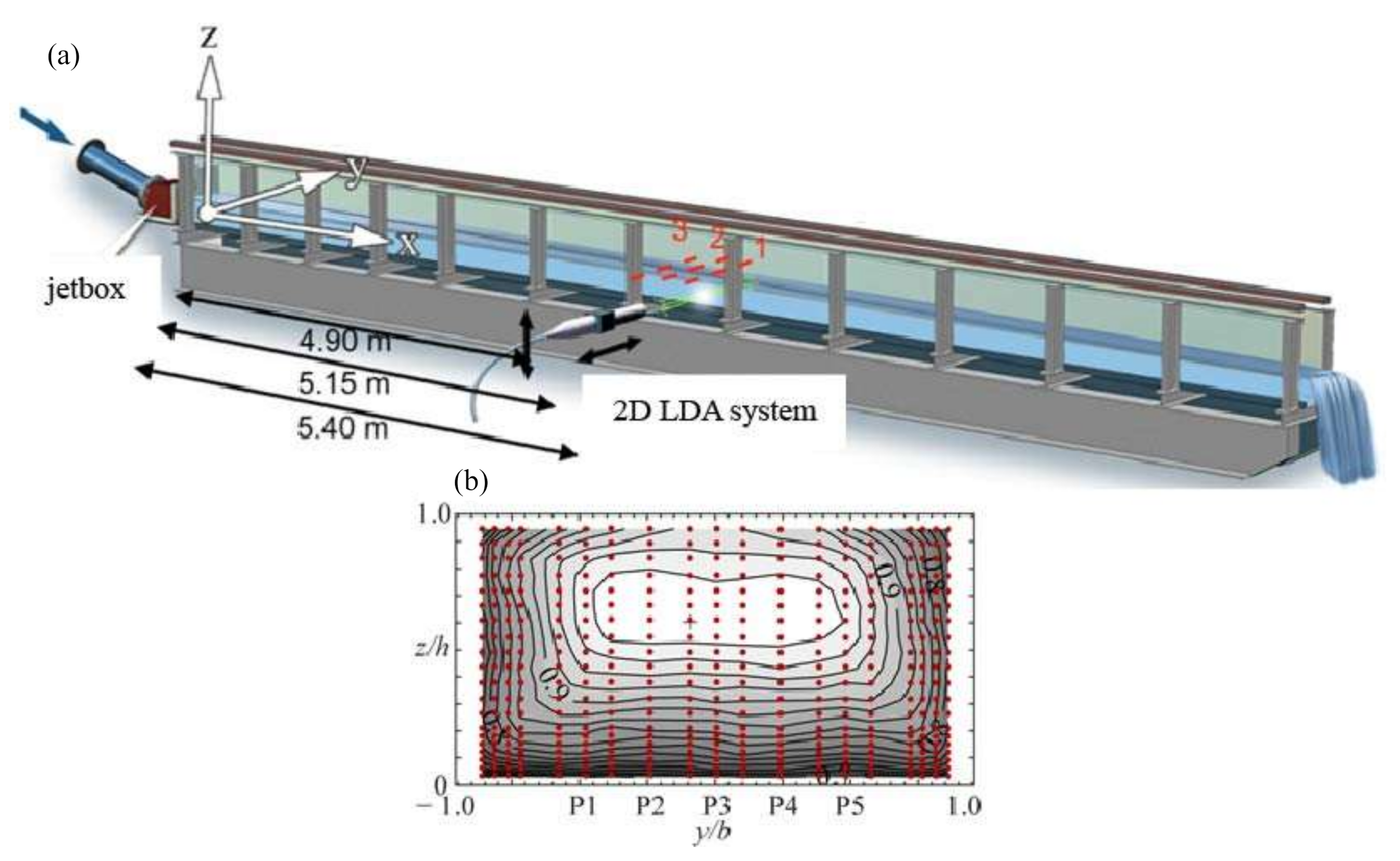
2. Experimental Setup

2.1. Laboratory Model Flume

The experiments were conducted in a b = 0.2 m wide, h_f = 0.5 m deep and l = 13.5 m long hydraulic model flume with a bed slope of S_b = 1%, representing a straight section of a SBT or SFC (Figure 1a). The flume bed was lined with a 20 cm thick concrete. The sidewalls were made of glass and wood. The pressurized pipe inflow was converted to free-surface flow into the flume with a jetbox system developed at the Laboratory of Hydraulics, Hydrology and Glaciology (VAW) of ETH Zurich [52]. The gate-controlled jetbox enables to adjust the approach flow depth h_o. The discharge Q was measured using a magnetic flow meter mounted to the pipe with ±0.5% measurement error. The flow depth h was measured at 0.5 m intervals along the flume, both using a point gauge and ultrasonic distance sensor (UDS) of ±0.5 mm data accuracy.

The x, y, and z coordinates represent the streamwise, transverse, and vertical directions, respectively (Figure 1a). The instantaneous flow velocities in streamwise and vertical directions are u = U + u’ and w = W + w’, respectively. Herein, U and W are the time averaged velocities while u’ and w’ denote the fluctuating velocities. The instantaneous velocities were measured using a 2D LDA with a 3D traverse system allowing LDA movements in each direction. At x = 5.40 m, 19 vertical velocity profiles (the red dots in Figure 1b), and at x = 5.15 m and 4.90 m, 5 vertical velocity profiles (P1–P5 in Figure 1b) were measured. The transverse spacing of the profiles was 5–15 mm across the flume and each profile consisted of 20–21 points, resulting in a total of 580–609 measuring points depending on the flow depth. The data acquisition frequency varied depending on the measurement location in the flume and it reached up to 4 kHz in the vicinity of the bottom. Recording time was set to 30 s at each measurement point. Due to the LDA system limitations, 2D data acquisition were made at z ≥ 12 mm, whereas only 1D velocity measurements were made in the streamwise direction between 3 mm < z ≤ 12 mm where the vertical beams hit the flume bed.

2.2. Test Conditions

Table 1. Experiments with corresponding hydraulic parameters at the first measurement cross-section (x = 5.40 m).

Test	Fo	F	ho	h	b/ho	b/h	R	${\overline{\mathit{U}}}_{\mathit{b}\mathit{u}\mathit{l}\mathit{k}}$	$\overline{\mathit{U}}$	$\frac{\overline{\mathit{U}}}{{\overline{\mathit{U}}}_{\mathit{b}\mathit{u}\mathit{l}\mathit{k}}}$	β
	(-)	(-)	(cm)	(cm)	(-)	(-)	(105)	(m/s)	(m/s)	(-)	(-)
TA1	2.0	1.9	10	10.5	2	1.91	4.0	1.95	1.96	1.01	−0.80
TA2	3.0	2.5	10	11.2	2	1.79	5.6	2.66	2.68	1.01	−0.43
TA3	4.0	3.3	10	11.4	2	1.75	7.5	3.52	3.52	1.00	−0.26
TA4	2.0	1.9	15	16.0	1.33	1.25	5.7	2.31	2.31	1.00	−0.69
TA5	3.0	2.6	15	16.6	1.33	1.21	8.3	3.31	3.30	1.00	−0.35
TA6	4.0	3.3	15	17.0	1.33	1.17	10.8	4.30	4.42	1.03	−0.21
TA7	3.0	2.6	20	22.3	1	0.90	10.5	3.79	3.85	1.02	−0.30
TA8	3.5	3.0	20	22.4	1	0.89	12.1	4.39	4.47	1.02	−0.23

shows the experimental matrix and summarizes the experimental conditions. Experiments were coded as TA1–TA8. In contrast to TA1–TA6, the Froude numbers of TA7 and TA8 were limited to F_o = 3 and 3.5 due to the limitations of jetbox and experimental flume. In all the test runs, the roughness Reynolds number was k_s⁺ < 5, and hence the flow regime was hydraulically smooth (Equation (5)). The cross-sectional averaged flow velocities $\overline{U}$ were determined using the continuity equation, in which the discharge was determined using two methods: (I) bulk cross-sectional averaged flow velocity, i.e., ${\overline{U}}_{bulk}=Q/(b\cdot h)$, calculated with the discharge Q, which is measured by the magnetic flow meter, and (II) averaged flow velocity $\overline{U}$ calculated from the LDA measurements as $\overline{U}=Q/A$ with $Q={\displaystyle \int U}dA$, where A = wetted flow area, and U = time averaged velocities at each measurement point. These values are in a good agreement with a maximum 3% difference (Table 1).

The flow was gradually varied; therefore, the water level measurements were used to calibrate the backwater curve, which was calculated with Δx = 0.05 m intervals along the flume to determine the flume friction losses and quantify the energy line slope S_e as well as the uniform sand roughness height k_s. The flow equilibrium parameter β denoting the flow uniformity degree is computed with [53]:

$$\beta =\frac{g{R}_h}{U_{*l}^2}\left(\frac{d{R}_h}{dx}-S_b\right)$$

(11)

herein, R_h = A/P = bh/(b + 2h) = hydraulic radius, P = wetted perimeter, and U_*l = spatially averaged friction velocity, which was calculated by averaging the local friction velocities determined with the log-law fits of 19 individual velocity profiles at x = 5.40 m. The value of β = −1 represents uniform flow, while β > −1 and β < −1 denote decelerated and accelerated flows, respectively. In this study, the flow was decelerated in each test run with β > −1 (Table 1). Therefore, the approach flow parameters such as F_o, h_o, U_o, R_o and b/h_o at x = 0 differ from those at x = 5.40 m, i.e., F, h, U, R, and b/h, respectively (Table 1).

3. Experimental Results and Discussion

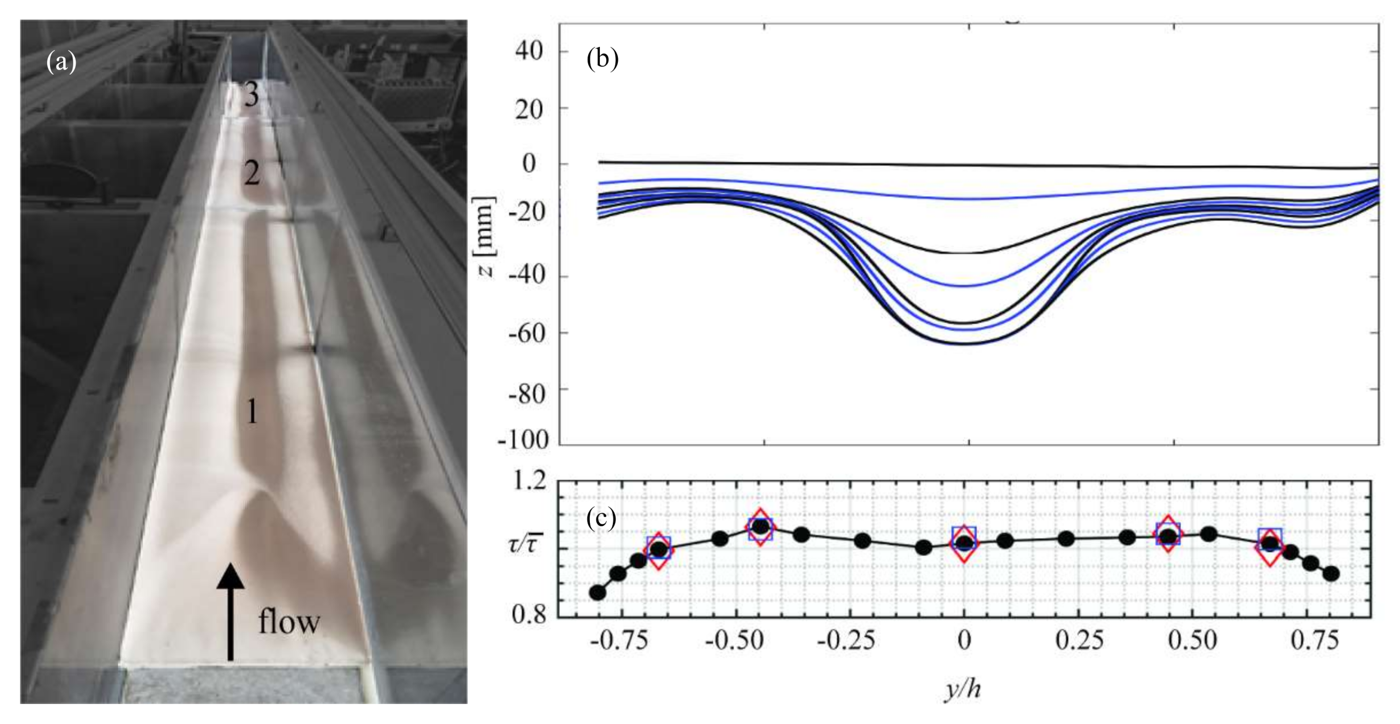
3.1. Mean Flow Characteristics

We first examine the effect of aspect ratio on the mean flow velocities for b/h_o = 1, 1.33, and 2. Figure 2, Figure 3 and Figure 4 show the contour lines of the mean streamwise (U) and vertical (W) velocities normalized by the maximum streamwise flow velocity (U_max) with the idealized sketches of the secondary currents across the flume for test runs TA1–TA3, TA4–TA6 and TA7 and TA8, respectively. The results show that the streamwise and vertical flow velocities have a quasi-symmetrical distribution over the transverse direction with U_max (illustrated by “+”) in the centerline for all test runs except TA1 with a slight shift (Figure 2, Figure 3 and Figure 4). The mean streamwise and vertical flow velocity distributions reveal a well-developed stationary free-surface vortex near the water surface (Figure 2a, I = free-surface vortex), a bottom vortex near the bed (Figure 2a, IV = bottom vortex), and one pair of vortices between the free-surface and bottom vortices at the each half of the flume (Figure 2a, II and III = mid-vortices or mid vortex pairs). These vortices cause bulging of the contour lines of the streamwise velocities with respect to the water surface (Figure 2a, A = surface corner bisector) and the bottom corner bisectors (Figure 2a, C = bottom corner bisector). The mid-vortices bulge the streamwise contours towards the flume center up to approx. y/h = ±0.60, ±0.20 and ±0.10 for TA1–TA3, TA4–TA6 and TA7 and TA8, respectively. The mid-vortices confine the free-surface vortices and prevent them to extend down to the bottom vortex region for TA1–TA8. The free-surface vortices transfer momentum and energy from the side walls to the flume center near the water surface. The transfer continues from there towards mid-flow depth with a strong downward flow causing the velocity dip phenomenon (Figure 2, Figure 3 and Figure 4). Hence, the maximum flow velocities are well below the water surface from approximately z/h = 0.65 down to z/h = 0.50 with decreasing aspect ratio from TA1 to TA8, respectively. The boundary between the mid-vortices (Figure 2a, B = mid-bisector) in the transverse direction corresponds to the vertical locations of the maximum velocities except TA2–TA3. It is evident that increasing the Froude number from TA1 to TA3 (Figure 2), TA4 to TA6 (Figure 3) and TA7 to TA8 (Figure 4) does not affect the vortex patterns but decreases the aspect ratios due to increasing flow non-uniformity (See β values in Table 1), enhancing vortices with stronger bulging of streamwise velocity contour lines.

Figure 2, Figure 3 and Figure 4 also show that with decreasing aspect ratio, the size of the mid and the bottom vortices increases towards the flume center. In addition, the height of the free-surface vortices also increases and reaches the mid-water column at the flume center. Furthermore, the width of the high flow velocity zone narrows in the transverse direction, while it enlarges in the vertical direction with decreasing aspect ratio. Overall, secondary currents with four well-developed streamwise vortices at each half of the flume significantly change the mean flow velocity distributions with strong up- and down-flows. Their strength and size increase with decreasing aspect ratio.

3.2. Logarithmic Law & Friction Velocities

The semi-logarithmic plots of the mean streamwise velocity profiles U⁺(z⁺) with the corresponding classical log-law fit (Equation (1)) and modified log-wake-law fit (MLWL) (Equation (9)) at x = 4.90, 5.15, and 5.40 m and y/h = 0 (center axis) are shown in Figure 5a–c for TA1–TA3, TA4–TA6, and TA7 and TA8, respectively. The von Kármán and integral constants obtained from the fits are κ = 0.41, and A = 5.29, respectively. The log-law without wake function (Equation (1)) agrees well with the experimental data in the wall region z/h ≤ 0.2 independent of the Froude number and non-uniform decelerated flow conditions [6,12,14,54]. The log-fits even extend in the outer region up to z/h ≈ 0.3 for TA1–TA3, whereas it holds only in the wall region, i.e., z/h ≤ 0.2 for TA4–TA8. This clearly indicates the secondary current effect on the log-fits. Similar results are reported by [14] for aspect ratios 2.5 ≤ b/h ≤ 2.8 in supercritical open channel flows. In 3D flows, the results from [12,14] as well as the present study indicate that a velocity dip correction in addition to the log-law is necessary to estimate the velocity profile in the whole water column [55]. To this end, the MLWL was applied to our data, which resulted in good correlations with large coefficient of determination values, R² ≥ 0.97 (Figure 5). The values of α and Π determined from the fit of Equation (9) are in a range of 0.49 ≤ α ≤ 0.81 and 0.18 ≤ Π ≤ 0.42, respectively (

Table 2. Ratios of apparent shear stresses at the water surface to bed shear stresses (α), wake parameters (Π), and mean friction velocities calculated using bed slope, energy line slope, and logarithmic fittings.

Test	α	Π	U*b (m/s)	U*e (m/s)	U*l (m/s)	β (-)
TA1	0.513	0.241	0.071	0.077	0.080	−0.80
TA2	0.492	0.355	0.072	0.104	0.104	−0.43
TA3	0.518	0.332	0.073	0.136	0.134	−0.26
TA4	0.686	0.325	0.078	0.089	0.090	−0.69
TA5	0.751	0.399	0.078	0.124	0.124	−0.35
TA6	0.802	0.415	0.079	0.165	0.161	−0.21
TA7	0.614	0.185	0.082	0.144	0.144	−0.30
TA8	0.622	0.262	0.082	0.166	0.162	−0.23

). These values vary depending on the aspect ratio and are in good agreement with literature data [14,16,22,37]. However, the relationship between the present Π values and the flow non-uniformity parameter β (Table 1), i.e., the pressure gradient, was not proportional (Table 2), as stated by [37,39]. Such difference may be attributed to the determination of the velocity dip location, which directly affects the wake parameter.

Friction velocity, also called “shear velocity”, is a fictive velocity representing the bed shear stress in velocity units and is an essential parameter in sediment transport and erosion related problems. In uniform flow conditions, the flume average friction velocity based on the channel bed slope (U_*b) is calculated with the following equation:

$$U_{*b}=g{R}_h{S}_b$$

(12)

where S_b = channel bed slope. In non-uniform flows, the flume average friction velocity U_*e can be calculated using energy line slope S_e instead of S_b in Equation (12). In addition to these two methods, the local friction velocity u_*l can be determined from the log-law fits (Equation (1)). Spatially averaged friction velocities U_*l are calculated by averaging the local friction velocities u_*l determined from each vertical velocity profiles. These three methods were applied to the present measured data, and the obtained average friction velocities U_*b, U_*e, U_*l, are listed in Table 2. The comparison of the friction velocities (Table 2) shows that the U_*e and U_*l values match well, whereas U_*b values are lower. This is expected and attributed to the effect of the non-uniform flow conditions where the channel bed and the energy line slopes differ. The closer β is to unity, the better U_*b agrees with U_*e and U_*l. These results suggest that the spatially averaged friction velocity in non-uniform open channel flows can be calculated using Equation (12) with S_e even at such low aspect ratios in case of lack of velocity data.

3.3. Turbulent Flow Characteristics

3.3.1. Cross-Sectional Turbulence Intensity Distributions

Streamwise and vertical turbulence intensities u_rms and w_rms are the root-mean-square values of the fluctuating velocities u′ and w′, respectively, and calculated as

$$u_{rms}=\sqrt{\overline{u^{\prime 2}}},w_{rms}=\sqrt{\overline{w^{\prime 2}}}$$

(13)

Figure 6 presents the contour lines of the u_rms and w_rms normalized with the cross-sectional mean friction velocity (U_*l) for the test runs TA1–TA3. The cross-sectional distributions of u_rms and w_rms are symmetrical with respect to the flume center for these test runs. Both the streamwise and vertical turbulences are generated near the flume bed and the side walls, showing higher values near the boundaries. They decrease towards the locations of the velocity-dip phenomenon (Figure 6). Both u_rms and w_rms are higher in the up-flow region and, side flow between the mid-vortices from the side wall to the flume center, while they are low in the down-flow regions (Figure 6 and Figure 2d–f). The most notable feature observed from Figure 6 is that the secondary currents affect the cross-sectional distributions of u_rms and w_rms more pronouncedly compared to the mean streamwise flow velocity distributions for all test runs (Figure 2 vs. Figure 6). The contour lines of u_rms are quasi-symmetrical with respect to the bottom corner bisector whereas they are asymmetric along the free-surface bisectors with strong bulging towards the top corners (Figure 6a–c). The magnitudes of u_rms near the bed and the sidewall are similar and support the observed symmetries in the corner bisector regions. On the contrary, the contour lines of w_rms reveal asymmetrical distributions with respect to both bottom corner and surface bisectors. Furthermore, the magnitudes of w_rms are higher near the side walls compared to those near the bed, which is different than those for u_rms.

At lower aspect ratios from 1.25 (TA4) to 0.89 (TA8) (Figure 7 and Figure 8), the effect of the secondary currents on the turbulence intensities follows similar but more pronounced patterns as described for TA1–TA3. The region of the minimum values of u_rms and w_rms enlarges in vertical direction and narrows in a transverse direction with decreasing aspect ratio because of the stronger free-surface vortices and the mid-vortices (black colored regions in Figure 6, Figure 7 and Figure 8). Such trend is similar to that observed for the distribution of the streamwise flow velocities (Figure 2, Figure 3 and Figure 4).

3.3.2. Vertical Distributions of Turbulence Intensities

Figure 9a–c show the vertical profiles of normalized streamwise turbulence intensities u_rms/u_*l for all the measurements at x = 4.90, 5.15, and 5.40 m and y/h = 0 (centerline) for TA1–TA3, TA4–TA6, and TA7 and TA8, respectively. Figure 9 also shows the universal turbulence intensity equation for 2D open-channel flows [12]:

$$u_{rms}/u_{*l}=2.3e^{(-z/h)}$$

(14)

The streamwise turbulence intensities are highest near the bottom, and gradually decrease while following the relation given in Equation (14) up to z/h ≈ 0.5 for TA1–TA3 (Figure 9a). Above this point, they sharply decrease and deviate from Equation (14) towards the water surface, reaching its minimum at around z/h ≈ 0.6–0.7, where the velocity dip phenomenon occurs (Figure 9a). Above z/h > 0.7, they increase again towards the water surface and intersect with Equation (14). Such deviations from Equation (14) in the outer region, i.e., z/h > 0.5 are caused by the strong secondary currents. Due to the decreasing aspect ratio, these currents push the deviation points from Equation (14) towards the flume bed down to z/h ≈ 0.30 for TA4–TA6 (Figure 9b) and z/h ≈ 0.20 for TA7 & TA8 (Figure 9c). Below these elevations, streamwise turbulence intensities follow Equation (14) for TA4–TA8. The minimum values of u_rms/u_*l occur in the regions of 0.5 < z/h < 0.7 for TA4–TA6, and 0.6 < z/h < 0.8 for TA7 and TA8 corresponding to the expansion of maximum velocity area (velocity dip) in the vertical direction (Figure 3 and Figure 4). The present data show that despite flow non-uniformity, the streamwise turbulence intensities match well at three streamwise locations along the flume at each aspect ratio (Figure 9). Reference [14] found similar results for 2.5 ≤ b/h ≤ 2.8.

Figure 10a–c show the vertical profiles of normalized vertical turbulence intensities w_rms/u_*l for all the measurements at x = 4.90, 5.15, and 5.40 m and y/h = 0 (centerline) for TA1–TA3, TA4–TA6, and TA7 and TA8, respectively. The universal vertical turbulence intensity function for 2D open channel flows is also shown in Figure 10 [12]:

$$w_{rms}/u_{*l}=1.27e^{(-z/h)}$$

(15)

The vertical turbulence intensities are highest near the flume bed and also higher than Equation (15). They follow the similar trends described for the streamwise turbulence intensities for all measurements with an exception of a slight Froude number effect for TA1–TA6. Increasing Froude number causes flow deceleration, i.e., increasing β value, hence resulting in a slightly decreased aspect ratio. As a result, w_rms values are higher in the wall region and lower in the outer region with increasing β. The former effect is also observed by [52] for decelerating 2D flows, whereas the latter effect occurs because of the strong secondary currents. The effect of Froude number on w_rms is negligible for TA7 and TA8. In all runs, the data match well at three streamwise locations at the flume center for each aspect ratio.

Ref. [14]’s data only slightly show the effect of secondary currents on w_rms for the aspect ratios of 2.5 ≤ b/h ≤ 2.8. A comparison between their data and the present data reveals that the secondary current effect on w_rms is pronounced for b/h < 2.5 as the side wall effects on the flow become more dominant.

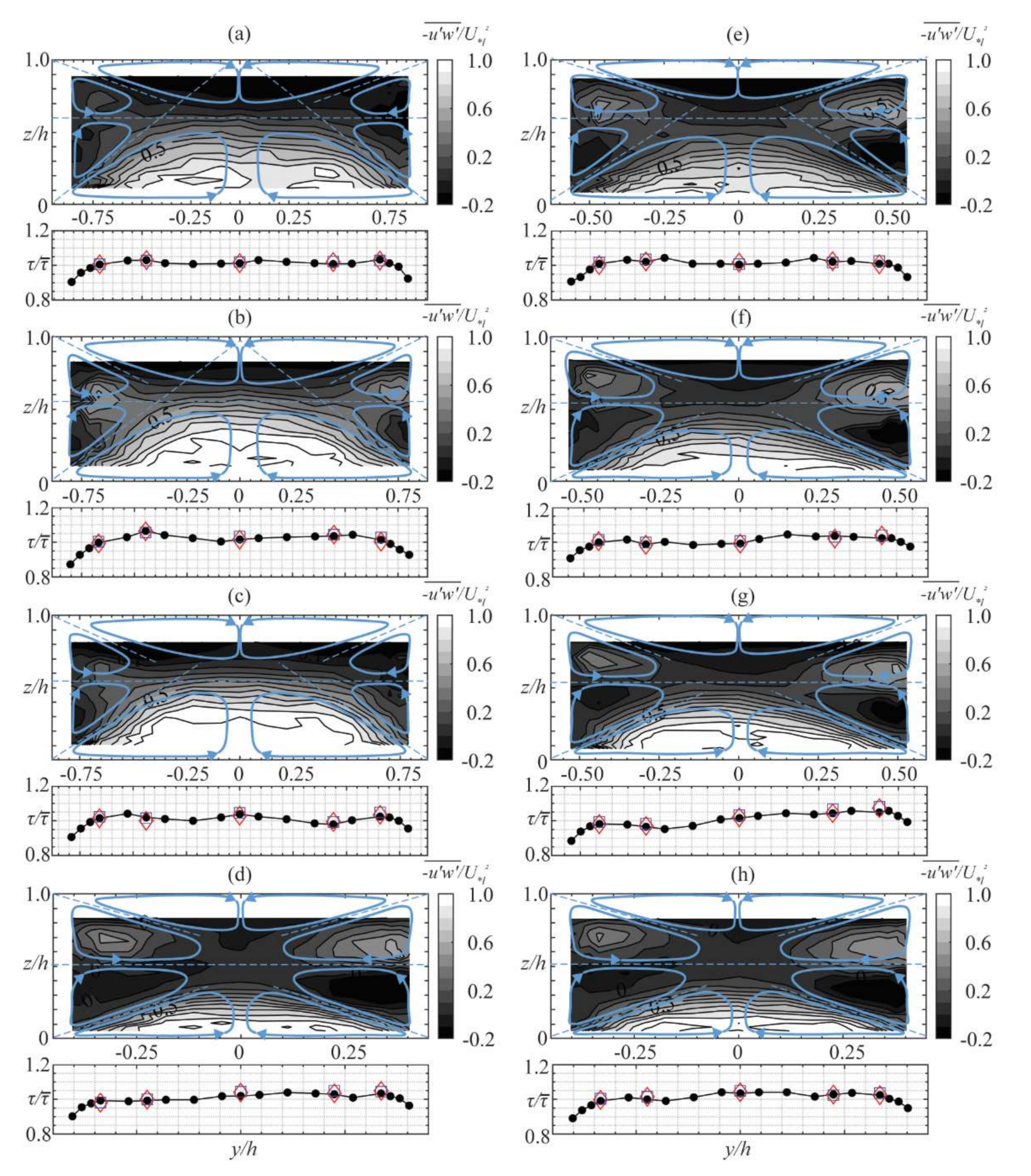
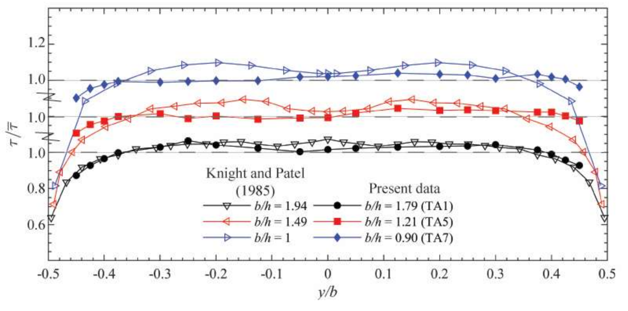
3.3.3. Reynolds and Bed Shear Stress Distributions

This section presents the cross-sectional distributions of Reynolds shear stress $-\overline{u´w´}$ at x = 5.40 m, and the transverse variation of bed shear stress, τ normalized by its average value $\overline{\tau }$ at x = 4.90, 5.15, and 5.40 m. The bed shear stresses were calculated using the local friction velocities obtained from the logarithmic fits:

$$\tau =\rho u_{*l}^2$$

(16)

where ρ = water density. Figure 11 presents the contour lines of the Reynolds shear stresses ($-\overline{u´w´}$) normalized by the square of the cross-sectional averaged friction velocity (U_*l²) together with the corresponding transverse distribution of the normalized bed shear stresses for the test runs TA1–TA3 (Figure 11a–c), TA4–TA6 (Figure 11e–g), and TA7 and TA8 (Figure 11d,h). The distributions of Reynolds shear stresses are consistent with the secondary current patterns derived from the streamwise and vertical mean flow velocities and turbulence intensities (Figure 2, Figure 3 and Figure 4 and Figure 6, Figure 7 and Figure 8). As also stated in previous studies [12,14,44,56], Reynolds shear stresses are higher in the up-flow regions of secondary currents corresponding to the flume center near the bed (W > 0) with the contours bulging towards the free surface. They are lower in the down-flow regions (W < 0) close to the flume sidewalls near the bed with the contours bulging towards the bed for all tests (Figure 11). The Reynolds shear stresses are negative at the free-surface region, where the streamwise velocity gradient is also negative, i.e., ∂U/∂z < 0 due to the impact of free-surface vortices. Similarly, the Reynolds shear stresses are negative and positive at the core of the lower and upper mid-vortices, respectively, and become negative again close to the free surface near each sidewall. Such changes correspond to the changes of ∂U/∂z (Figure 2, Figure 3 and Figure 4).

The normalized bed shear stresses are lowest near the sidewalls and reach maxima around y/h = 0.50–0.6, 0.50, and 0.25–0.30 for TA1–TA3, TA4–TA6, and TA7 and TA8, respectively. From these points on, they flatten or slightly reduce towards the flume center for all aspect ratios (Figure 11). This pattern is similar to those reported by [10,57] for similar aspect ratios and differ from the data by [14], which shows the maximum bed shear stress even closer to the sidewalls for aspect ratios of 2.5, 2.6, and 2.8. The difference between the minimum and maximum bed shear stresses in the present study is approximately 0.30$\overline{\tau }.$ The bed shear stress distributions at three different measurement cross-sections x = 4.90, 5.15, and 5.40 m match well with a maximum difference of 4%, indicating that the flow deceleration due to increasing Froude number at each aspect ratio does not affect the transverse bed shear stress distribution in flow direction [12,14,44,58]. The bed shear stress distributions correlate with the Reynolds shear stress distribution. Overall, it is evident that the strong secondary vortices at low aspect ratios significantly influence the Reynolds shear stresses, and hence the bed shear stress distributions. The resulting bed shear stress pattern is expected to affect the sediment transport (see the engineering application section below), particle dispersion, and mixing processes in the water column.

Figure 12a–c show the Reynolds shear stress profiles normalized by the square of the local friction velocity at three measurement cross-sections x = 4.90, 5.15, and 5.40 m at the flume center (y/h = 0) with the universal fit for 2D flows ($-\overline{u´w´}$/u_*² = 1 – z/h) for TA1–TA8. Due to the strong secondary currents, the Reynolds shear stress distributions deviate from the linear distribution. For small z/h values, the deviation is positive and convex shaped due to the up-flow bottom vortices. The maximum Reynolds shear stresses occur at around z/h = 0.20, 0.15 and 0.10 for TA1–TA3, TA4–TA6 and TA7 and TA8, respectively. This behavior can be attributed to the stronger free-surface vortices with the decreasing aspect ratio, i.e., the down-flow region extending from the free surface towards the channel bed, and hence limits the up-flow region generated by the bottom vortices. Therefore, the Reynolds shear stresses decrease down to zero at the location of velocity dips, i.e., U = U_max, depending on the aspect ratio. Above the velocity dip location, Reynolds shear stresses become negative and decrease towards the free surface for all test runs because of the negative velocity gradient (∂U/∂z < 0). The present data also reveal that the Froude number slightly influences the Reynolds shear stress distributions for similar aspect ratios. Therefore, the Froude number effect is negligible as reported in [12,14]. These findings are similar to those determined for turbulence intensities (Figure 9 and Figure 10).

3.4. Engineering Example

The objective of the present research project described in the introduction is to develop a realistic mechanistic hydro-abrasion prediction model by determining the interrelation among the flow characteristics, sediment transport modes, and hydro-abrasion with systematic laboratory investigations. Abrasion tests were conducted in the same experimental flume using erodible foam and mortar as bed lining materials to investigate the time development of hydro-abrasion depth and patterns in a straight SBT section. These tests were made under the same hydraulic conditions as detailed in Table 1 by varying the sediment characteristics as hardness, shape, size, and the sediment supply rate on different bed lining materials of various strengths. Details of the foam properties used in the experiments such as specific mass (ρ_f), splitting tensile strength (f_st), compressive strength (f_c), and elasticity (Young’s) modulus (Y_M) are listed in

Table 3. Bed lining material properties used in hydro-abrasion experiments.

Foam Type	ρf (kg/m3)	fst (MPa)	fc (MPa)	YM (MPa)
low-strength foam	64	0.32	0.36	3.92
medium-strength foam	96	0.50	0.60	5.38
high-strength foam	128	0.84	0.92	10.33

.

The first abrasion test was conducted at h_o = 10 cm and F_o = 3 (identical hydraulic conditions with TA2), using three different types of foam by placing them in series according to their strengths from the highest to the lowest (Figure 13a). As abrasive material, natural particles of mean diameter D_m = 6 mm were used at various sediment supply rates of Q_s = 100, 200, 400, and 700 g/s. In the experiment, a sediment mass of M_s ≈ 3840 kg was used to abrade the foam at Q_s = 100 g/s. After this step, the sediment amount was reduced to half, i.e., M_s ≈ 1920 kg for each supply rate while the latter was increased to Q_s = 200, 400, and 700 g/s to accelerate the total run time. In order to determine the abraded volumes and calculate the depths along the flume, the flume bed was scanned using a Leica P15 model laser scanner at the initial condition as well as certain time steps corresponding to half the amount of total sediment mass released for each Q_s. Figure 13a shows the abraded channel bed after the test, while Figure 13b shows the temporal development of spatially averaged cross-sectional profiles of the medium-strength foam at eight different time steps (t = 5.3, 10.6, 11.9, 13.2, 13.9, 14.5, 14.9, 15.2 h) with the corresponding bed shear stress distribution at the initial condition, t = 0 (Figure 13c). The initial abrasion profile matches well with the bed shear stress distribution with higher abrasion depth at the flume center and lower abrasion depths at the flume sidewalls (Figure 13b,c). In time, abrasion concentrated at the flume center with increasing depth and width. Such results indicate that: (I) the bottom vortices carry more sediment at the flume center with high bed shear stress (Figure 11), and (II) the development of a center incision channel moves these vortices towards the flume center in time and makes them stable herein. In return, bottom vortices increase bed shear stress, transport more sediment, and cause higher abrasion depths at the flume center compared to the flume sidewalls.

4. Comparison with Literature

Secondary currents of Prandtl’s second kind occurring in straight narrow open-channel flows, i.e., with aspect ratio, b/h < 4–5 are an important phenomenon superimposing themselves on the primary flow. They affect the distribution of longitudinal velocities, turbulence intensities, Reynolds and bed shear stresses, thus influencing the sediment transport, and the 3D bed formation [12]. The present experimental results confirm such effects of the secondary currents on the flow field and show that four vortex pairs, i.e., free-surface vortices, two mid-vortices, and bottom vortices formed for all studied hydraulic parameters. This secondary current pattern differs from that reported by [12] with one stronger free-surface vortex and one bottom vortex, i.e., two vortices at each half of the flume for similar b/h_o = 2. The present aspect ratios of b/h = 1.91, 1.79 and 1.75, and the Froude numbers of F = 1.9, 2.5 and 3.3 are slightly lower than b/h = 2 and higher than F = 0.54 and 1.22 in [12], respectively. Such difference between the studies suggests that b/h = 2 is a critical aspect ratio: below this value, a strong free-surface vortex breaks into three smaller vortices (Figure 2, Figure 3 and Figure 4). It is also likely that higher Froude numbers may also affect the development of more vortices due to the increasing free-surface roughness. [14] observed such rough surface for F_o ≥ 4 and high air-entrainment at F_o = 8. Decreasing aspect ratio from 1.91 (TA1) down to 0.89 (TA8) enhances secondary currents and substantially affects the turbulent flow characteristics in return. Since no detailed velocity measurements at such low aspect ratios in open channel flow are available, we visited an experimental study in a rectangular duct flow conducted by [59] using an LDA. Figure 14 compares the normalized streamwise velocity and Reynolds shear stress distributions of the present data of TA8 and [59] with b/h = 0.89 and b/h = 1, respectively. Velocity and Reynolds shear stress magnitudes differ between two studies because of the pressurized flow, as well as the different boundary conditions in the duct flow. However, the flow and Reynolds shear stress patterns are similar, particularly in the lower half of the channel, i.e., between z/h = 0 and 0.5. In the upper half of the channel, the patterns slightly differ because the solid top boundary in the duct creates symmetrical flow patterns, whereas the free surface in the present case creates asymmetrical flow patterns with regard to the horizontal axis at z/h ≈ 0.5. In both open channel and duct flows, Reynolds shear stresses are higher at the core region of the mid-vortices with changing signs depending on the vortex location. They are zero at the horizontal axis between mid-vortices, where the longitudinal velocity gradient, i.e., ∂U/∂z, changes its sign. At the vertical boundary between the bottom vortices at flume center, the Reynolds shear stresses are not zero. Furthermore, since the boundary layer grows from the channel bed, the positive Reynolds shear stress region occupies more space than the negative shear stress region in the lower half of the channel. The maximum shear stress in the latter region is much smaller than that in the former region. The only difference between the duct and open channel flows is that such structures are symmetrical in the duct flow whereas they are asymmetrical in the open channel flow (Figure 14b). In the latter case, shear stresses are higher at the core of the closed region of the upper mid-vortex compared to that at the core of the lower mid-vortex (Figure 14b). Despite some differences explained, the overall pattern and the effect of secondary currents on the turbulent flow characteristics in both flow types are similar at such a low aspect ratio, for which the effect of side walls becomes more dominant in open-channel flows.

In addition to the experimental studies, [10] simulated turbulence-driven secondary currents for open-channel and duct flows with various aspect ratios using a mathematical model. The model results show that (I) the free-surface vortices shrink and the bottom vortices grow in size and strength with decreasing b/h, (II) the corner induced bottom vortices grow and become more dominant for b/h < 2, and (III) the surface vortices increase in dimensions, but cannot preserve their strength and are split into several weaker vortices for b/h < 1. The present study shows completely different flow patterns than those reported by [10] for similar aspect ratios, indicating that their model does not correctly simulate secondary currents. Reference [10] also pointed out that they could not validate their results with experimental data, and hence such data were desirable. The present study addresses this issue by providing high-resolution experimental data for calibration and validation of mathematical and 3D numerical models.

Secondary currents affect bed shear stresses. Depending on the aspect ratio, their distribution shows different patterns. [57] stated that the maximum bed shear stress occurs towards the side walls for intermediate aspect ratios 1 < b/h < 5. [14,41] confirmed such patterns for the aspect ratios 2 < b/h < 5. In contrast to [57], the present data show that the bed shear stress is minimum near the sidewalls and increases towards the flume center for aspect ratios 0.89 ≤ b/h ≤ 1.91 (Figure 15). [60]’s results for airflows in a rectangular duct confirm our findings with a slight deviation only for an aspect ratio of 0.90 (Figure 15). Note that in the literature, data comparison between open-channel and duct flows is based on half of the aspect ratio of the former for the latter, i.e., b/h for the former versus b/2h for the latter, which is not applied here. At low aspect ratios where the flume side walls strongly affect the flow field as in the present study, such an approach used in the literature could cause misinterpretation of the results. Therefore, we suggest our approach to be used for the data comparison at low aspect ratios.

5. Conclusions

Herein, we report the results of a systematic experimental study on the effects of secondary currents on the turbulence characteristics of supercritical open channel flows at very low aspect ratios over a smooth fixed bed—a first to our knowledge. We conducted detailed 2D LDA velocity measurements in a laboratory flume with a 1% bed slope. The main studied hydraulic parameters were the aspect ratios b/h_o = 1–2 and the approach flow Froude numbers, F_o = 2–4. The flow conditions were both quasi-uniform and gradually varied depending on the Froude number and aspect ratio.

Our study demonstrates that eight well-developed turbulence-driven secondary currents, i.e., free-surface and bottom vortex pairs, and two mid-vortex pairs in between, occur in the flume cross section without any bed forms. The secondary current flow pattern is clearly visible in the cross-sectional distributions of the mean streamwise and vertical flow velocities, turbulence intensities and Reynolds and bed shear stress distributions. The mean vertical flow velocities with up- and down-flows at the side walls and the flume centers match well with the secondary current pattern. Strong down-flow near the water surface and up-flow near the flume bed at the flume center correspond to the accelerated, and decelerated regions of streamwise velocity, respectively. Therefore, the maximum velocity occurs well below the water surface, which is called "velocity-dip phenomenon". Hence, the logarithmic Prandtl-von Kármán type velocity distribution (log-law) requires a velocity dip correction in the outer region. A recently developed modified log-wake-law including this correction applies well to our data in both the inner and outer regions for all studied hydraulics conditions and thus is recommended for 3D flows as in the present study.

Secondary currents significantly change the distributions of Reynolds shear stress and turbulence intensities resulting in an undulation in the water column as observed in the mean velocity distributions. Higher and lower shear stresses and turbulence intensities occur in the down and up flow regions of secondary currents, respectively. The vertical distribution of both Reynolds shear stress and turbulence intensities at the flume center deviate from the universal laws applied for 2D flows.

Bed shear stresses accurately determined from the log-fits show an undulated pattern in the transverse direction. They are the lowest near the sidewalls, reach maxima, and then flatten or slightly reduce towards the flume center for all aspect ratios. This pattern is associated with the existence of the bottom vortices and vice versa, and also revealed for the distribution of Reynolds and turbulence intensities in the water column. Such pattern does not exist for the aspect ratios >2. Therefore, the aspect ratio of two is assumed to be a threshold value, differentiating the bed shear stress distribution in the transverse direction. The average bed shear stresses calculated from the log-fits and the simple energy line slope approach are in good agreement. Therefore, if no velocity data is available, it is recommended to use the latter approach for gradually varied 3D flows.

The effect of the aspect ratio on the dynamics of the secondary currents is pronounced. Decreasing the aspect ratio does not change the number and overall pattern of secondary currents but increase the strength of secondary currents. Furthermore, they shift the location of the maximum velocity further down from the water surface, reaching the mid-flume depth at the lowest aspect ratio of 0.89.

The Froude and Reynolds numbers do not affect the number and pattern of the secondary currents for a given aspect ratio. Increasing the Froude number causes decelerating flow, and hence slightly decreasing aspect ratio along the flume. Despite this, the normalized vertical distributions of streamwise mean flow velocity, turbulence intensities, and Reynolds shear stresses measured at three streamwise locations match quasi-well, indicating no or only a weak effect of Froude number on these quantities.

The pattern of secondary currents and their effect on flow quantities are similar to those obtained from duct flow measurements. However, they deviate from previous experimental and numerical open channel flow studies for similar aspect ratios. For this reason, we recommend our data for calibration and validation of numerical and mathematical model studies.

Overall, the findings of the present study provide a quite comprehensive characterization of 3D highly supercritical flows at very low aspect ratios. They contribute to a better understanding of the secondary current dynamics and their potential effects on the bed shear stresses, and hence sediment transport as well as hydro-abrasion mechanism occurring in hydraulic structures and steep bedrock rivers. The present study is expected to underpin the follow-up of studies on the effects of various bed roughness on the secondary currents at similar hydraulic conditions.

References

1. Boes, R.M.; Hagmann, M. Sedimentation countermeasures—Examples from Switzerland. In Proceedings of the First International Workshop on Sediment Bypass Tunnels, Zurich, Switzerland, 27–29 April 2015. [Google Scholar]
2. Micheletti, N.; Lane, S.N. Water yield and sediment export in small, partially glaciated Alpine watersheds in a warming climate. Water Resour. Res. 2016, 52, 4924–4943. [Google Scholar] [CrossRef] [Green Version]
3. Delaney, I.; Bauder, A.; Huss, M.; Weidmann, Y. Proglacial erosion rates and processes in a glacierized catchment in the Swiss Alps. Earth Surf. Process. Landf. 2018, 43, 765–778. [Google Scholar] [CrossRef] [Green Version]
4. Sklar, L.S.; Dietrich, W.E. A mechanistic model for river incision into bedrock by saltating bed load. Water Resour. Res. 2004, 40. [Google Scholar] [CrossRef]
5. Turowski, J.M. Stochastic modeling of the cover effect and bedrock erosion. Water Resour. Res. 2009, 45. [Google Scholar] [CrossRef] [Green Version]
6. Auel, C. Flow Characteristics, Particle Motion and Invert Abrasion in Sediment Bypass Tunnels. Ph.D. Thesis, ETH Zurich, Zürich, Switzerland, 2014. [Google Scholar]
7. Auel, C.; Albayrak, I.; Sumi, T.; Boes, R.M. Sediment transport in high-speed flows over a fixed bed: 1. Particle dynamics. Earth Surf. Process. Landf. 2017, 42, 1365–1383. [Google Scholar] [CrossRef]
8. Auel, C.; Albayrak, I.; Sumi, T.; Boes, R.M. Sediment transport in high-speed flows over a fixed bed: 2. Particle impacts and abrasion prediction. Earth Surf. Process. Landf. 2017, 42, 1384–1396. [Google Scholar] [CrossRef]
9. Müller-Hagmann, M.; Albayrak, I.; Auel, C.; Boes, R.M. Field investigation on hydroabrasion in high-speed sediment-laden flows at sediment bypass tunnels. Water 2020, 12, 469. [Google Scholar] [CrossRef] [Green Version]
10. Naot, D.; Rodi, W. Calculation of secondary currents in channel flow. J. Hydraul. Div. 1982, 108, 948–968. [Google Scholar]
11. Tominaga, A. Nezu, lehisa Velocity profiles in steep open-channel flows. J. Hydraul. Eng. 1992, 118, 73–90. [Google Scholar] [CrossRef]
12. Nezu, I.; Nakagawa, H. Turbulence in Open-Channel Flows; IAHR-AIRH monograph series; Balkema: Rotterdam, The Netherlands, 1993; ISBN 978-90-5410-118-5. [Google Scholar]
13. Albayrak, I.; Auel, C.; Boes, R.M. Supercritical flow in sediment bypass tunnels. In Proceedings of the 12th International Symposium on River Sedimentation, Kyoto, Japan, 2–5 September 2013; pp. 1867–1875. [Google Scholar]
14. Auel, C.; Albayrak, I.; Boes, R.M. Turbulence characteristics in supercritical open channel flows: Effects of Froude number and aspect ratio. J. Hydraul. Eng. 2014, 140, 4014004. [Google Scholar] [CrossRef]
15. Nikuradse, J. Strömungsgesetze in Rauhen Rohren [Flow Laws in Rough Pipes]; VDI-Verlag: Dusseldorf, Germany, 1933. [Google Scholar]
16. Nezu, I.; Rodi, W. Open-channel flow measurements with a laser Doppler anemometer. J. Hydraul. Eng. 1986, 112, 335–355. [Google Scholar] [CrossRef]
17. Cardoso, A.; Graf, W.H.; Gust, G. Uniform flow in a smooth open channel. J. Hydraul. Res. 1989, 27, 603–616. [Google Scholar] [CrossRef]
18. Lyn, D. Resistance in flat-bed sediment-laden flows. J. Hydraul. Eng. 1991, 117, 94–114. [Google Scholar] [CrossRef]
19. Kironoto, B.; Graf, W.H. Reynolds. Turbulence characteristics in rough non-uniform open-channel flow. Proc. Inst. Civ. Eng. Water Marit. Energy 1995, 112, 336–348. [Google Scholar] [CrossRef]
20. Von Kármán, T. Mechanische Ähnlichkeit und Turbulenz [Mechanical similarity and turbulence]. Math Phys. Kl. 1930, 5, 58–76. [Google Scholar]
21. Prandtl, L. Zur turbulenten Strömung in Rohren und längs Platten [On turbulent flows in ducts and along plates]. Ergeb. Aerodyn. Vers. Zu Gött. 1932, 4, 18–29. [Google Scholar]
22. Coles, D. The law of the wake in the turbulent boundary layer. J. Fluid Mech. 1956, 1, 191–226. [Google Scholar] [CrossRef] [Green Version]
23. Schlichting, H.; Gersten, K. Boundary-Layer Theory; Springer: Berlin/Heidelberg, Germany, 1979. [Google Scholar]
24. Bradshaw, P.; Huang, G.P. The law of the wall in turbulent flow. Proc. R. Soc. Lond. Ser. Math. Phys. Sci. 1995, 451, 165–188. [Google Scholar]
25. Prinos, P.; Zeris, A. Uniform flow in open channels with steep slopes. J. Hydraul. Res. 1995, 33, 705–719. [Google Scholar] [CrossRef]
26. Kırkgöz, M.S.; Ardıçlıoğlu, M. Velocity profiles of developing and developed open channel flow. J. Hydraul. Eng. 1997, 123, 1099–1105. [Google Scholar] [CrossRef]
27. Keramaris, E.; Pechlivanidis, G. Effects of different porous beds on turbulent characteristics in an open channel above the porous bed. Flow Meas. Instrum. 2017, 54, 20–26. [Google Scholar] [CrossRef]
28. Nikuradse, J. Gesetzmäßigkeiten der turbulenten Strömung in glatten Rohren Forsch [Laws of turbulent flows in smooth ducts]. Ing. Wesen. Bd 1932, 356, 1–36. [Google Scholar]
29. Shockling, M.; Allen, J.; Smits, A. Roughness effects in turbulent pipe flow. J. Fluid Mech. 2006, 564, 267. [Google Scholar] [CrossRef]
30. Langelandsvik, L.; Kunkel, G.; Smits, A.J. Flow in a commercial steel pipe. J. Fluid Mech. 2008, 595, 323. [Google Scholar] [CrossRef] [Green Version]
31. Bailey, S.C.; Vallikivi, M.; Hultmark, M.; Smits, A. Estimating the value of von Kármán’s constant in turbulent pipe flow. J. Fluid Mech. 2014, 749, 79. [Google Scholar] [CrossRef] [Green Version]
32. Hama, F.R. Boundary layer characteristics for smooth and rough surfaces. Trans. Soc. Nav. Arch. Mar. Engrs. 1954, 62, 333–358. [Google Scholar]
33. Colebrook, C.F.; Blench, T.; Chatley, H.; Essex, E.; Finniecome, J.; Lacey, G.; Williamson, J.; Macdonald, G. Turbulent flow in pipes, with particular reference to the transition region between the smooth and rough pipe laws (includes plates). J. Inst. Civ. Eng. 1939, 12, 393–422. [Google Scholar] [CrossRef]
34. Busse, A.; Thakkar, M.; Sandham, N.D. Reynolds-number dependence of the near-wall flow over irregular rough surfaces. J. Fluid Mech. 2017, 810, 196–224. [Google Scholar] [CrossRef] [Green Version]
35. Duan, J.G. Simulation of flow and mass dispersion in meandering channels. J. Hydraul. Eng. 2004, 130, 964–976. [Google Scholar] [CrossRef]
36. Pu, J.H. Universal velocity distribution for smooth and rough open channel flows. J. Appl. Fluid Mech. 2013, 6, 413–423. [Google Scholar]
37. Guo, J. Modified log-wake-law for smooth rectangular open channel flow. J. Hydraul. Res. 2014, 52, 121–128. [Google Scholar] [CrossRef]
38. Tominaga, A.; Nezu, I.; Ezaki, K.; Nakagawa, H. Three-dimensional turbulent structure in straight open channel flows. J. Hydraul. Res. 1989, 27, 149–173. [Google Scholar] [CrossRef]
39. Nezu, I. Open-channel flow turbulence and its research prospect in the 21st century. J. Hydraul. Eng. 2005, 131, 229–246. [Google Scholar] [CrossRef]
40. Einstein, H.A.; Li, H. Secondary currents in straight channels. Eos Trans. Am. Geophys. Union 1958, 39, 1085–1088. [Google Scholar] [CrossRef]
41. Nezu, I.; Nakagawa, H.; Tominaga, A. Secondary Currents in a Straight Channel Flow and the Relation to Its Aspect Ratio; Springer: Berlin/Heidelberg, Germany, 1985; pp. 246–260. [Google Scholar]
42. Nezu, I.; Azuma, R. Turbulence characteristics and interaction between particles and fluid in particle-laden open channel flows. J. Hydraul. Eng. 2004, 130, 988–1001. [Google Scholar] [CrossRef]
43. Rodríguez, J.F.; García, M.H. Laboratory measurements of 3-D flow patterns and turbulence in straight open channel with rough bed. J. Hydraul. Res. 2008, 46, 454–465. [Google Scholar] [CrossRef]
44. Albayrak, I.; Lemmin, U. Secondary currents and corresponding surface velocity patterns in a turbulent open-channel flow over a rough bed. J. Hydraul. Eng. 2011, 137, 1318–1334. [Google Scholar] [CrossRef]
45. Wohl, E.E.; Merritt, D.M. Bedrock channel morphology. Geol. Soc. Am. Bull. 2001, 113, 1205–1212. [Google Scholar] [CrossRef]
46. Müller-Hagmann, M. Hydroabrasion by High-Speed Sediment-Laden Lows in Sediment Bypass Tunnels. Ph.D. Thesis, ETH Zurich, Zürich, Switzerland, 2017. [Google Scholar]
47. Nikuradse, J. Turbulente Stromung im Innern des rechteckigen offenen Kanals [Turbulent flow inside the rectangular open channels]. Forsch. Heft 1926, 281, 36–44. [Google Scholar]
48. Reece, G.J. A Generalized Reynolds-Stress Model of Turbulence. Ph.D. Thesis, University of London, London, UK, 1977. [Google Scholar]
49. Launder, B.E.; Reece, G.J.; Rodi, W. Progress in the development of a Reynolds-stress turbulence closure. J. Fluid Mech. 1975, 68, 537–566. [Google Scholar] [CrossRef] [Green Version]
50. Xinyu, L.; Changzhi, C.; Zengnan, D. Turbulent flows in smooth-wall open channels with different slope. J. Hydraul. Res. 1995, 33, 333–347. [Google Scholar] [CrossRef]
51. Chatanantavet, P.; Whipple, K.X.; Adams, M.A.; Lamb, M.P. Experimental study on coarse grain saltation dynamics in bedrock channels. J. Geophys. Res. Earth Surf. 2013, 118, 1161–1176. [Google Scholar] [CrossRef] [Green Version]
52. Schwalt, M.; Hager, W. Die Strahlbox [The jetbox]. Schweiz. Ing. Archit. 1992, 110, 547–549. [Google Scholar]
53. Song, T.; Chiew, Y.M. Turbulence measurement in nonuniform open-channel flow using Acoustic Doppler Velocimeter (ADV). J. Eng. Mech. 2001, 127, 219–232. [Google Scholar] [CrossRef]
54. Samie, M.; Marusic, I.; Hutchins, N.; Fu, M.K.; Fan, Y.; Hultmark, M.; Smits, A.J. Fully resolved measurements of turbulent boundary layer flows up to Reτ = 20000. J. Fluid Mech. 2018, 851, 391–415. [Google Scholar] [CrossRef] [Green Version]
55. Yang, S.-Q.; Tan, S.-K.; Lim, S.-Y. Velocity distribution and dip-phenomenon in smooth uniform open channel flows. J. Hydraul. Eng. 2004, 130, 1179–1186. [Google Scholar] [CrossRef]
56. Stoesser, T.; McSherry, R.; Fraga, B. Secondary currents and turbulence over a non-uniformly roughened open-channel bed. Water 2015, 7, 4896–4913. [Google Scholar] [CrossRef] [Green Version]
57. Knight, D.W.; Demetriou, J.D.; Hamed, M.E. Boundary shear in smooth rectangular channels. J. Hydraul. Eng. 1984, 110, 405–422. [Google Scholar] [CrossRef]
58. Tamburrino, A.; Gulliver, J.S. Large flow structures in a turbulent open channel flow. J. Hydraul. Res. 1999, 37, 363–380. [Google Scholar] [CrossRef]
59. Melling, A.; Whitelaw, J.H. Turbulent flow in a rectangular duct. J. Fluid Mech. 1976, 78, 289–315. [Google Scholar] [CrossRef]
60. Knight, D.W.; Patel, H.S. Boundary shear in smooth rectangular ducts. J. Hydraul. Eng. 1985, 111, 29–47. [Google Scholar] [CrossRef]
Figure 1. (a) Laboratory model flume and measurement cross-sections at x = 4.90, 5.15, and 5.40 m, and (b) detailed velocity measurement points (19 profiles at cross-section x = 4.90 m, 5 profiles P1–P5 at cross sections x = 5.15 and 5.40 m).
Water 12 03233 g001
Figure 2. Contour plots of mean normalized flow velocities in (ac) streamwise direction, (df) vertical direction for TA1–TA3. In (a) I = free-surface vortex, II and III = mid vortices, IV = bottom vortex, A = surface corner bisector, B = mid-bisector, C = bottom corner bisector.
Water 12 03233 g002
Figure 3. Contour plots of mean normalized flow velocities in (ac) streamwise direction, (df) vertical direction for TA4–TA6.
Water 12 03233 g003
Figure 4. Contour plots of mean normalized flow velocities in (a,b) streamwise direction, (c,d) vertical direction for TA7 and TA8.
Water 12 03233 g004
Figure 5. Mean streamwise velocity profiles together with log-law (Equation (1)) and modified log-wake-law (Equation (9)) fits for (a) TA1–TA3, (b) TA4–TA6, (c) TA7–TA8 in all cross-sections at y/h = 0.
Water 12 03233 g005
Figure 6. Contour plots of turbulence intensities in (ac) streamwise direction, (df) vertical direction for TA1–TA3.
Water 12 03233 g006
Figure 7. Contour plots of turbulence intensities in (ac) streamwise direction, (df) vertical direction for TA4–TA6.
Water 12 03233 g007
Figure 8. Contour plots of turbulence intensities in (a,b) streamwise direction, (c,d) vertical direction for TA7 and TA8.
Water 12 03233 g008
Figure 9. Normalized streamwise turbulence intensity profiles for (a) TA1–TA3, (b) TA4–TA6, (c) TA7–TA8 in all cross-sections and universal fit [12].
Water 12 03233 g009
Figure 10. Normalized vertical turbulence intensity profiles for (a) TA1–TA3, (b) TA4–TA6, (c) TA7–TA8 in all cross-sections and universal fit [12].
Water 12 03233 g010
Figure 11. Contour plots of normalized Reynolds shear stresses and normalized bed shear stresses for (ac) TA1–TA3, (eg) TA4–TA6, (d,h) TA7 and TA8 (measurements at ●: x = 5.40 m; : x = 5.15 m; : x = 4.90 m).
Water 12 03233 g011
Figure 12. Normalized Reynolds shear stress profiles for (a) TA1–TA3, (b) TA4–TA6, (c) TA7 and TA8 in all cross-sections and universal fit [12].
Water 12 03233 g012
Figure 13. (a) Photo of the abraded bed after the test with ho = 10 cm, Fo = 3, Qs = 100, 200, 400, 700 g/s and Dm = 7.2 mm (1, 2 and 3 refer to high-, medium-, and low-strength foams, respectively), (b) Cross-sectional profile development on medium-strength foam at certain time steps, total run time is 15.2 h, (c) Corresponding normalized bed shear stress distribution for initial condition.
Water 12 03233 g013
Figure 14. Comparison of duct (left halves) and open channel flows (right halves): Contour plots of normalized (a) streamwise flow velocities, and (b) Reynolds shear stresses.
Water 12 03233 g014
Figure 15. Comparison of duct and open channel flows: bed shear stress distributions across the channel.
Water 12 03233 g015