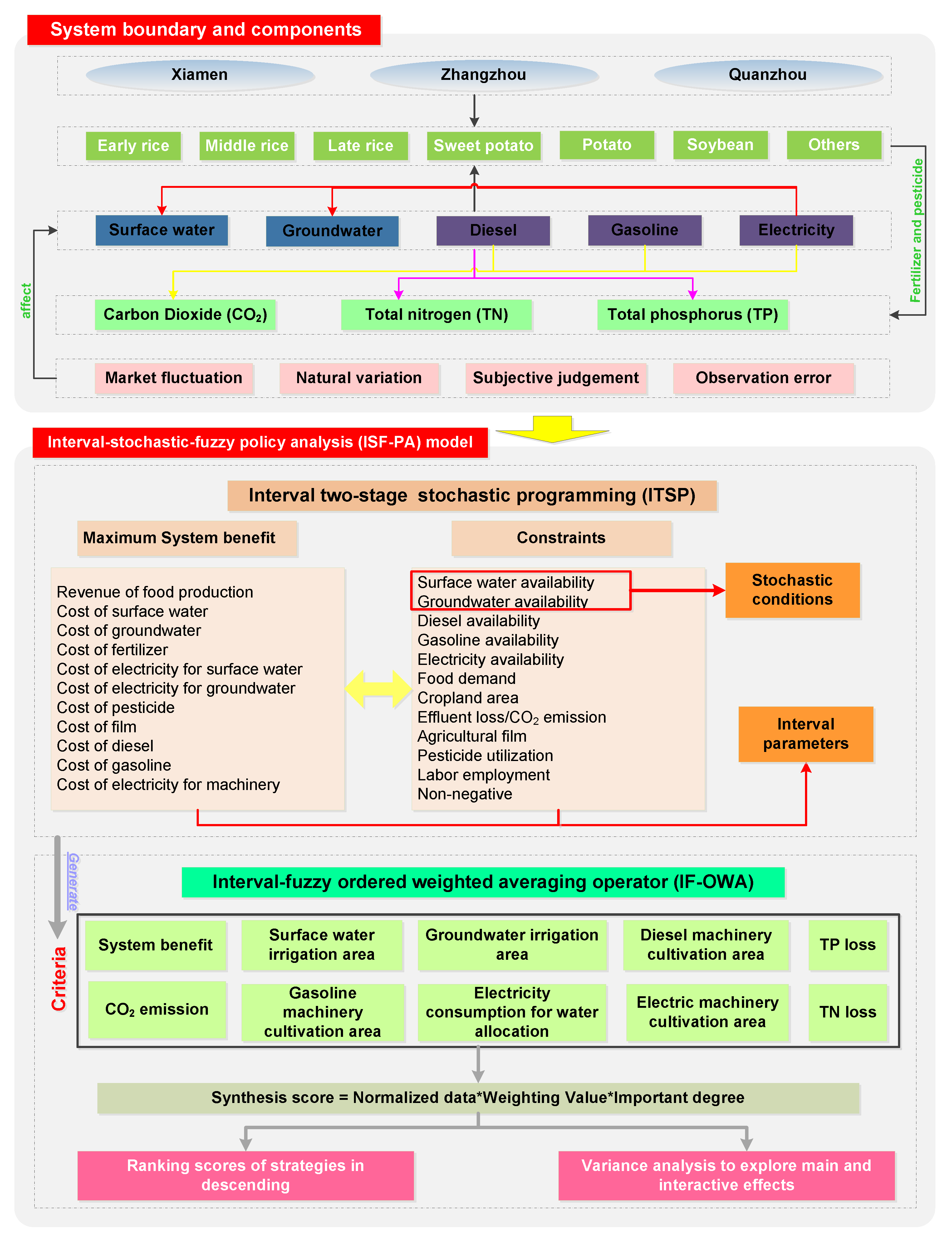
3.2. System Boundary and Components
Urban agglomeration is a complex system consisting of social, economic, environmental, and resource factors. An interval-stochastic-fuzzy policy analysis (ISF-PA) model which couples ITSP and IF-OWA models is formulated to support WEF security under multiple uncertainties. The framework of the ISF-PA model is presented in
Figure 2.
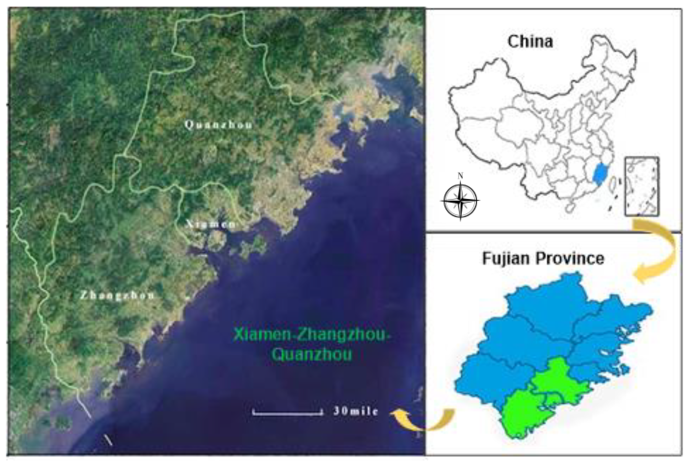
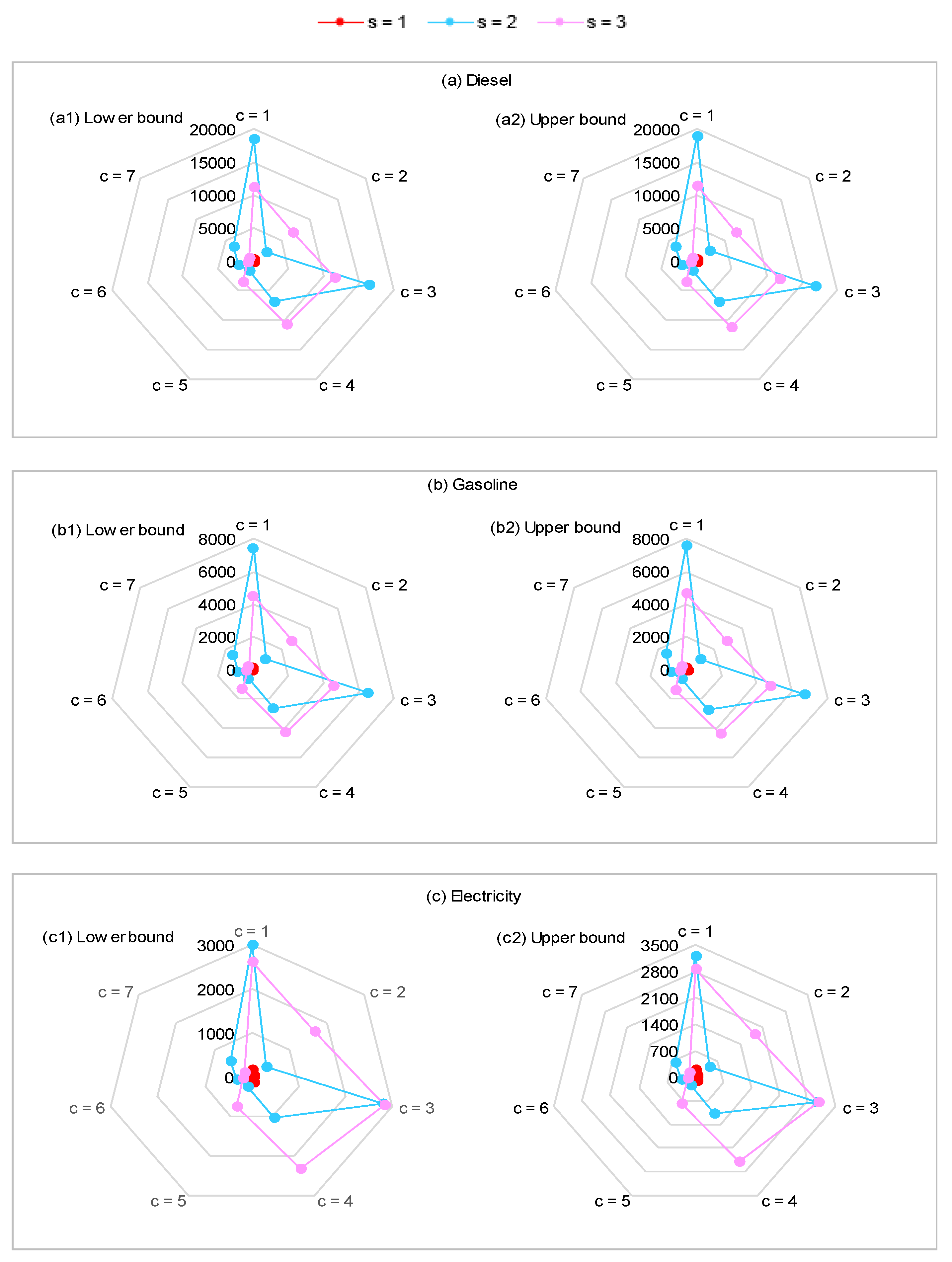
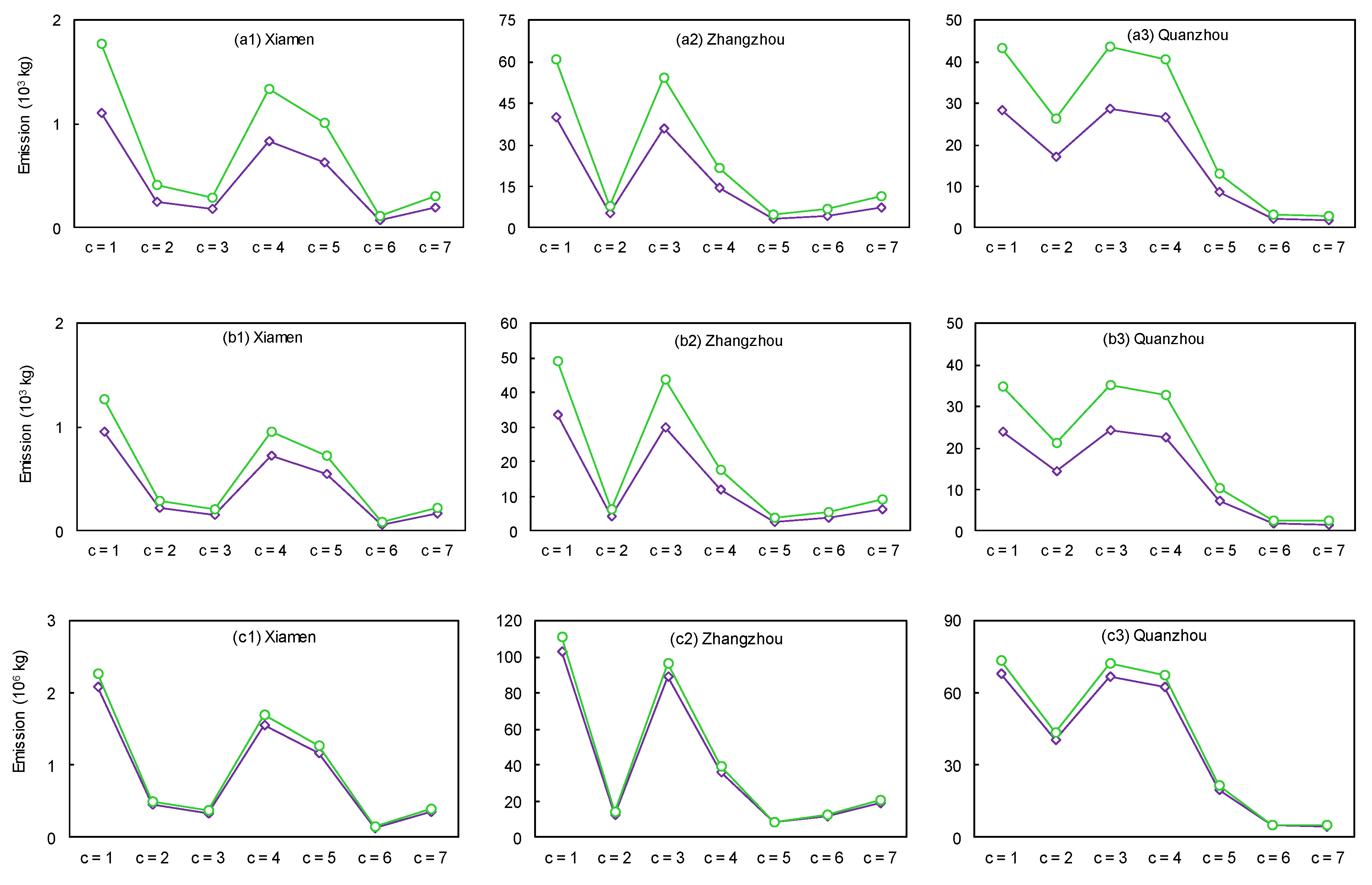
The study system is composed of (i) seven crops including early rice, middle rice, late rice, sweet potato, potato, soybean, and others; (ii) two water sources including surface water and groundwater; (iii) three energy sources including gasoline, diesel, and electricity; (iv) three emissions including carbon dioxide (CO2), total phosphorus (TP), and total nitrogen (TN); (v) two chemicals: pesticide and fertilizer; (vi) three cities: Xiamen, Zhangzhou, Quanzhou. Decision making processes should fully consider market situation, water requirement and availability for irrigation, electricity demand for water collection and delivery, energy demand for machinery operation, energy availability, land use policy, effluent and carbon emission, labor employment, and food guarantee, as well as represent the complexities and interactions among them. Meanwhile, economic and technological parameters vary with market fluctuations, subjective judgments of experts affect data acquisition and system reliability, spatiotemporal variability of runoff leads to changed available water resources, food demand increases with population growth, arable land area and food types affect energy consumption. The uncertainties are quantified as interval, stochastic, and fuzzy variables.
3.3. Modelling Formulation
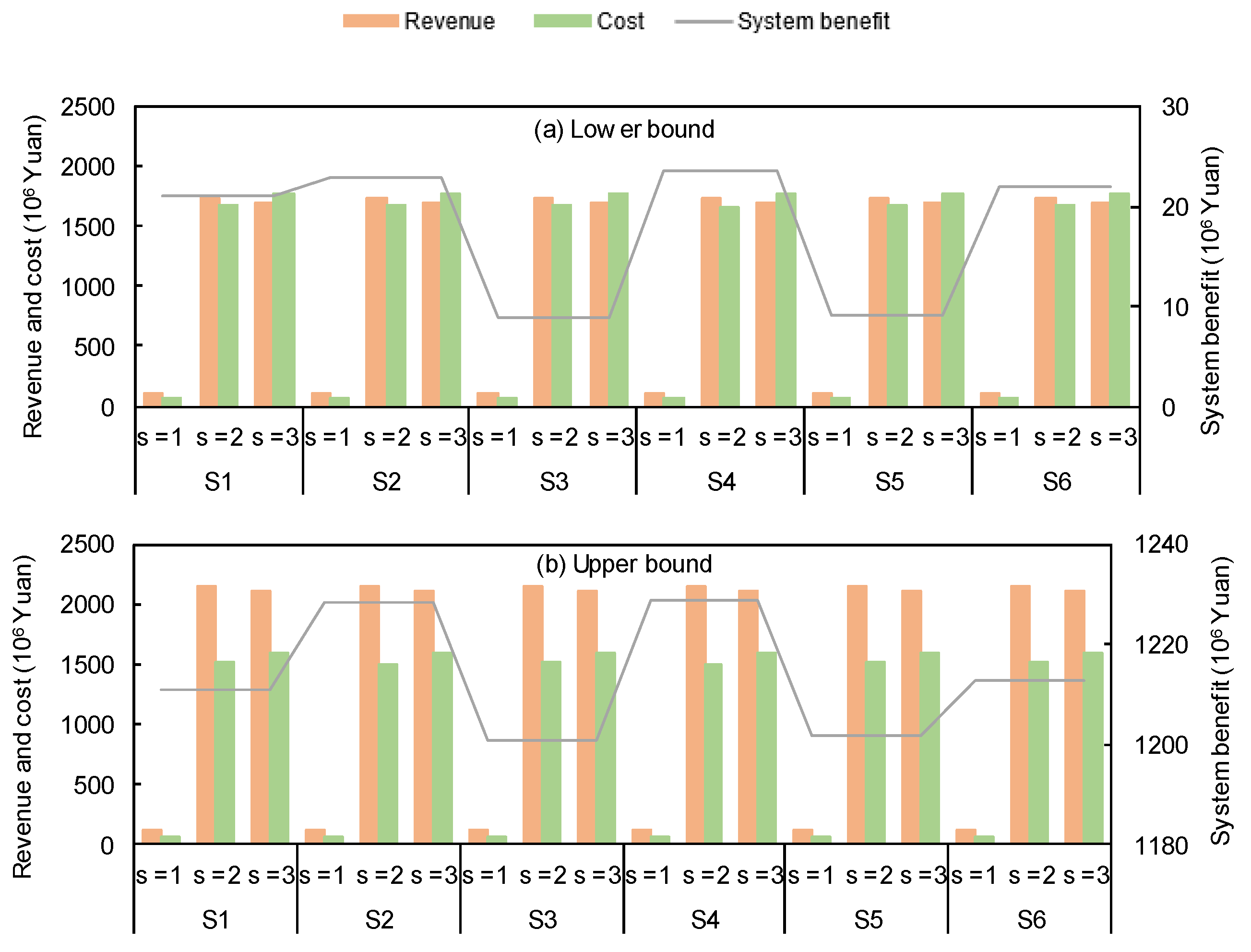
In the first stage, decision makers set initial targets of all crops in each city without catching available water resources conditions. In the second stage, random available water resources conditions are recognized. If targets are too high, local resources may not be sufficient to satisfy demand. Decision makers need to extract groundwater more deeply (which is harmful for aquifers). If targets are too low, local citizens may withstand economic losses. Infeasibilities in the second stage are allowed at a certain penalty (i.e., the second-stage decision is used to minimize penalty that may appear due to any infeasibility). A number of management policies related to cropland area, water allocation, and energy consumption can be obtained based on the ITSP model as follows:
Objective function:
where
c is index of crop;
s is index of city;
is available surface water level (
for low,
for medium,
for high);
is available groundwater level (
for low,
for medium,
for high);
is market price (Yuan/kg);
is lower bound of cropland area target that should be irrigated by water and cultivated by energy agricultural machine (ha);
is the difference between upper and lower bounds (ha);
is decision variables for destemming cropland area target in first-stage;
is unit crop yield (kg/ha);
is probability of available water occurrence under level
h;
is unit cost of surface water (Yuan/m
3);
is cropland area irrigated by surface water (ha);
is irrigation quota (m
3/ha);
is unit cost of groundwater (Yuan/m
3);
is cropland area irrigated by groundwater (ha);
is unit cost of fertilizer (kg/ha);
is unit cost of pesticide (Yuan/kg);
is unit cost of agricultural film (kg/ha);
is unit cost of diesel (Yuan/liter);
is unit diesel consumption of cropland (liter/ha);
is cropland area cultivated by diesel agricultural machinery (ha);
is cropland area cultivated by gasoline agricultural machinery (ha);
is cropland area cultivated by electric agricultural machinery (ha);
is unit cost of gasoline (Yuan/liter);
is unit gasoline consumption of cropland (liter/ha);
is unit cost of electricity (Yuan/kWh);
is unit electricity consumption for cropland (kWh/ha);
is unit electricity consumption for surface water (kWh/m
3);
is unit electricity consumption for groundwater (kWh/m
3);
Constraints:
(1) Surface water availability: Surface water delivered to all the crops in each city should not be higher than available surface water supply.
(2) Groundwater availability: Groundwater allocated to all the crops in each city should not be higher than allowable groundwater pumping.
(3) Energy availability: The energy consumption for crop cultivation should not be higher than the available energy for agriculture in each subarea.
(4) Food security: The yield of food grain for each subarea should satisfy the food grain requirement that is associated with population in order to guarantee food security.
(5) Cropland area: Cropland area should not be higher than the maximum value and lower than minimum value. All cropland should be irrigated by water and cultivated by energy agricultural machine.
(6) Total nitrogen emission: Nitrogen emission by fertilizer application should not be higher than the allowable amount.
(7) Total phosphorus emission: Phosphorus emission by fertilizer application should not be higher than the allowable amount.
(8) Agricultural film utilization: Agricultural film utilization often causes plastic environmental pollution, which needs to be controlled.
(9) Pesticide utilization: The spraying of pesticides often brings about COD and eutrophication environmental pollution, which must not exceed the allowable value.
(10) Carbon emission: Excessive CO
2 emission can lead to greenhouse effect. It is important to control CO
2 emission.
(11) Labor employment: The amount of labor is limited due to the budget.
(12) Non-negative variable: Since this is a real-world case study, all variables should be non-negative. Through running the proposed model, solutions of all decision variables can be obtained. System benefit can then be determined.
where
is available surface water (m
3);
is available groundwater (m
3);
is available diesel supply (liter);
is available gasoline supply (liter);
is available electricity supply (kWh);
is number of population (person);
is per food demand (kg/person);
is minimum cropland area (ha);
is maximum cropland area (ha);
is unit fertilizer application (kg/ha);
is total nitrogen content of fertilizer (kg N/kg);
is loss rate of total nitrogen (%);
is allowable total nitrogen loss (kg N);
is total phosphorus content of fertilizer (kg P/kg);
is loss rate of total phosphorus (%);
is allowable total phosphorus loss (kg N);
is unit agricultural film application (kg/ha);
is total allowable agricultural film application (t);
is unit pesticide application (kg/ha);
is total allowable pesticide application (t);
is carbon emission of diesel (kgCO
2/ liter);
is carbon emission of gasoline (kgCO
2/ liter);
is carbon emission of electricity (kgCO
2/kg);
is carbon emission of fertilizer (kgCO
2/kg);
is carbon emission of film (kgCO
2/kg);
is carbon emission of pesticide (kgCO
2/kg);
is total allowable carbon emission (kg);
is number of labor (person/ha);
is unit remuneration (Yuan/person);
is total remuneration (Yuan).
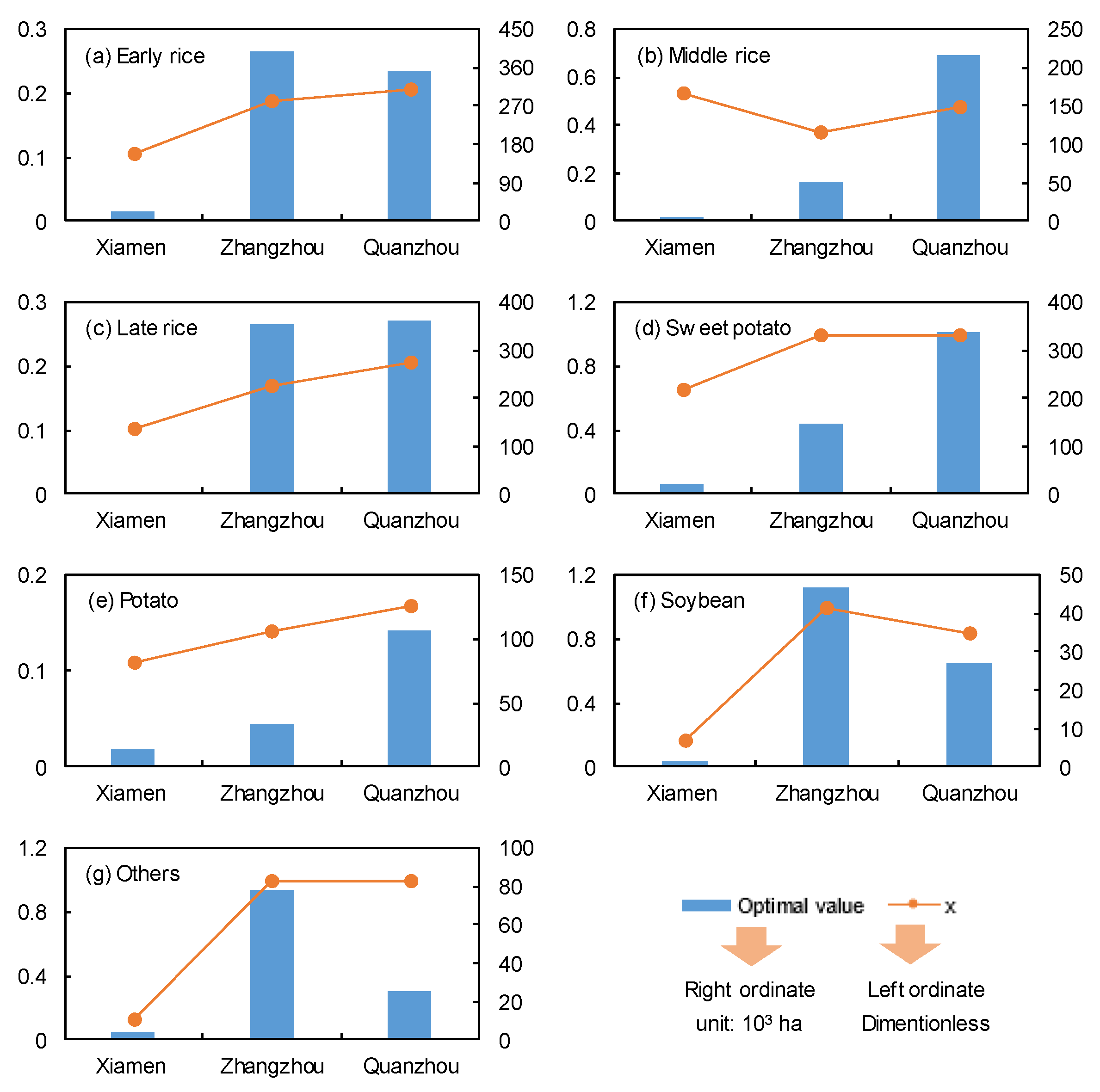
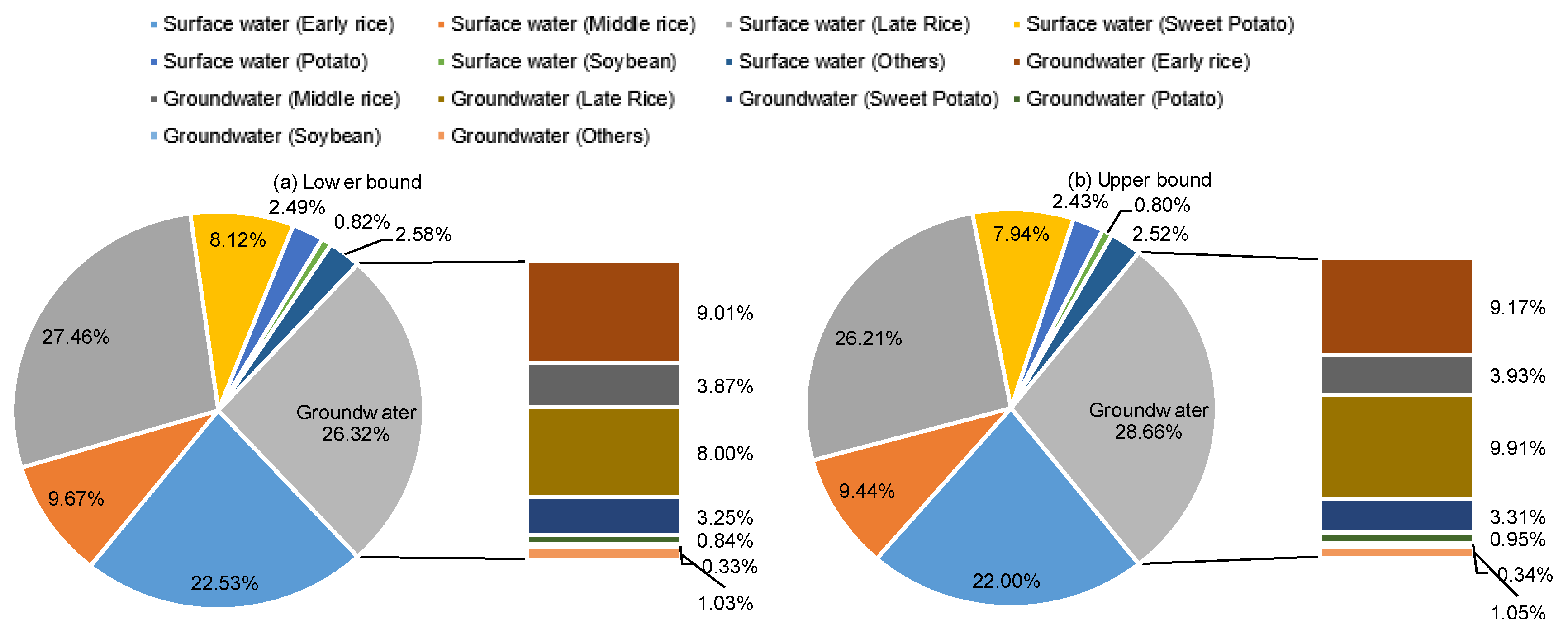
Table 1 shows the interval values of different cities and crops. Market prices were obtained from the “Agricultural Product Price Information Network of Fujian Province”; Crop yields were gained from “Statistical Yearbook” of each city; irrigation quotas were obtained from “Standard Local Water Quota of Fujian Province”; unit diesel, fertilizer, and pesticide application were extracted from “Agricultural Information Network” of the cities. Other parameters were obtained from field research and published references [
33,
45,
46].
Table 2 and
Table 3 present the values of stochastic surface water and groundwater (e.g., population growth and the expansion of urban areas impacted the groundwater level and its salinity, leading to changed groundwater availability) in the cities, which were collected from the “Water Resources Bulletin” of the cities [
47,
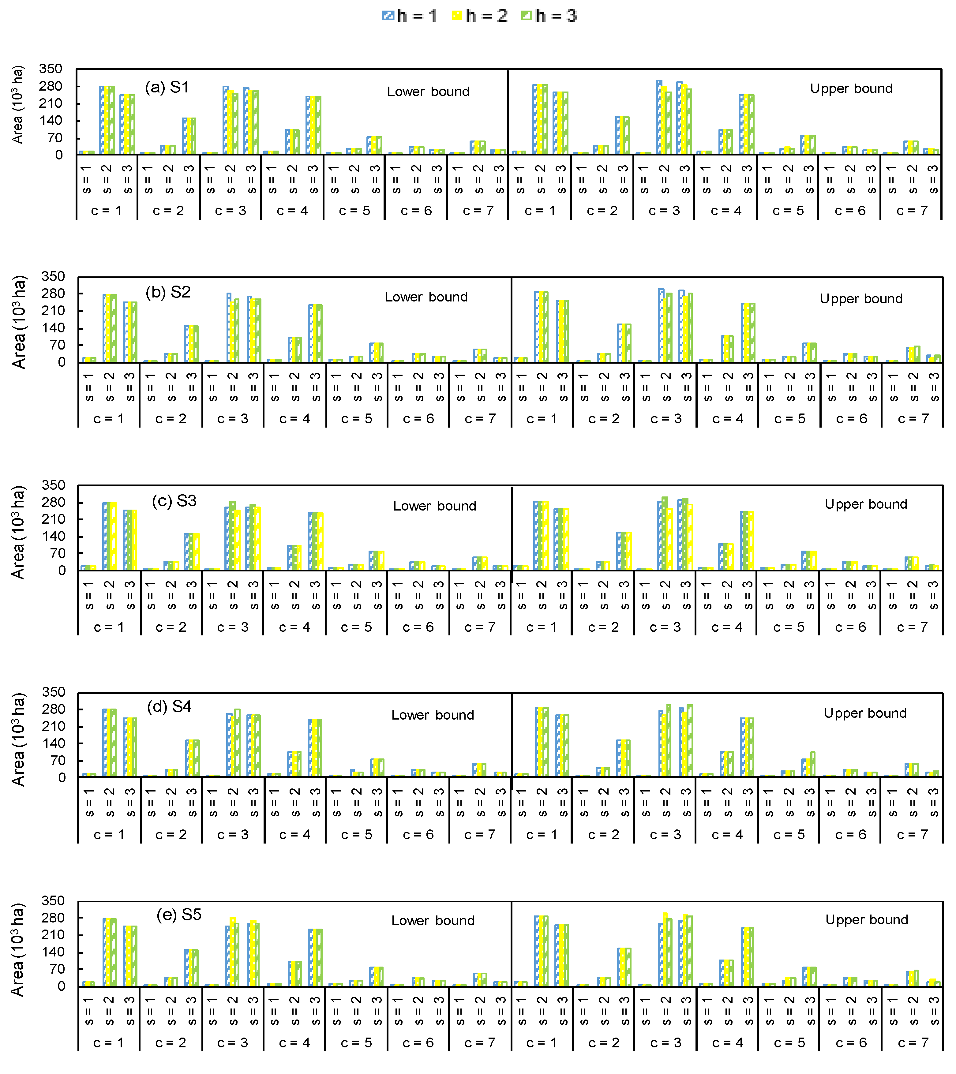
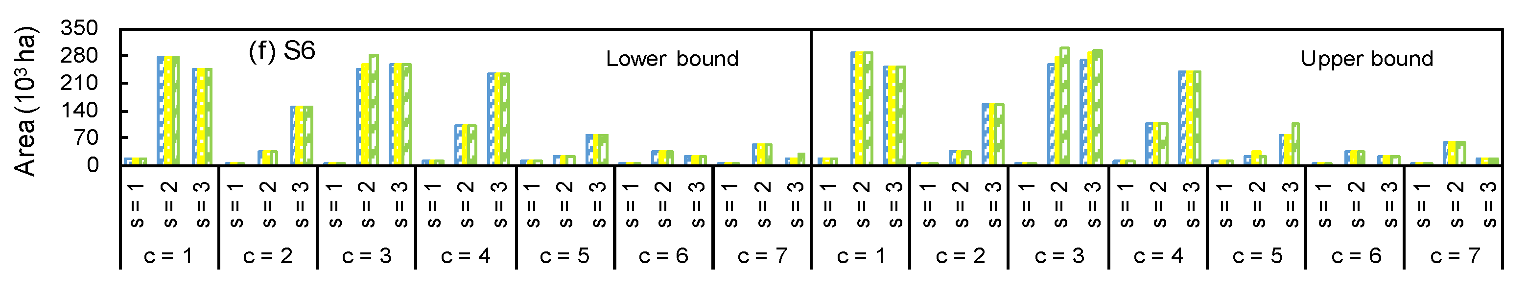
48]. Combinations of different available surface water and groundwater levels lead to six scenarios. For instance, for scenario 1 (i.e., S1), low (
), medium (
), and high (
) levels of surface water correspond to low (
), high (
), medium (
) levels of groundwater.
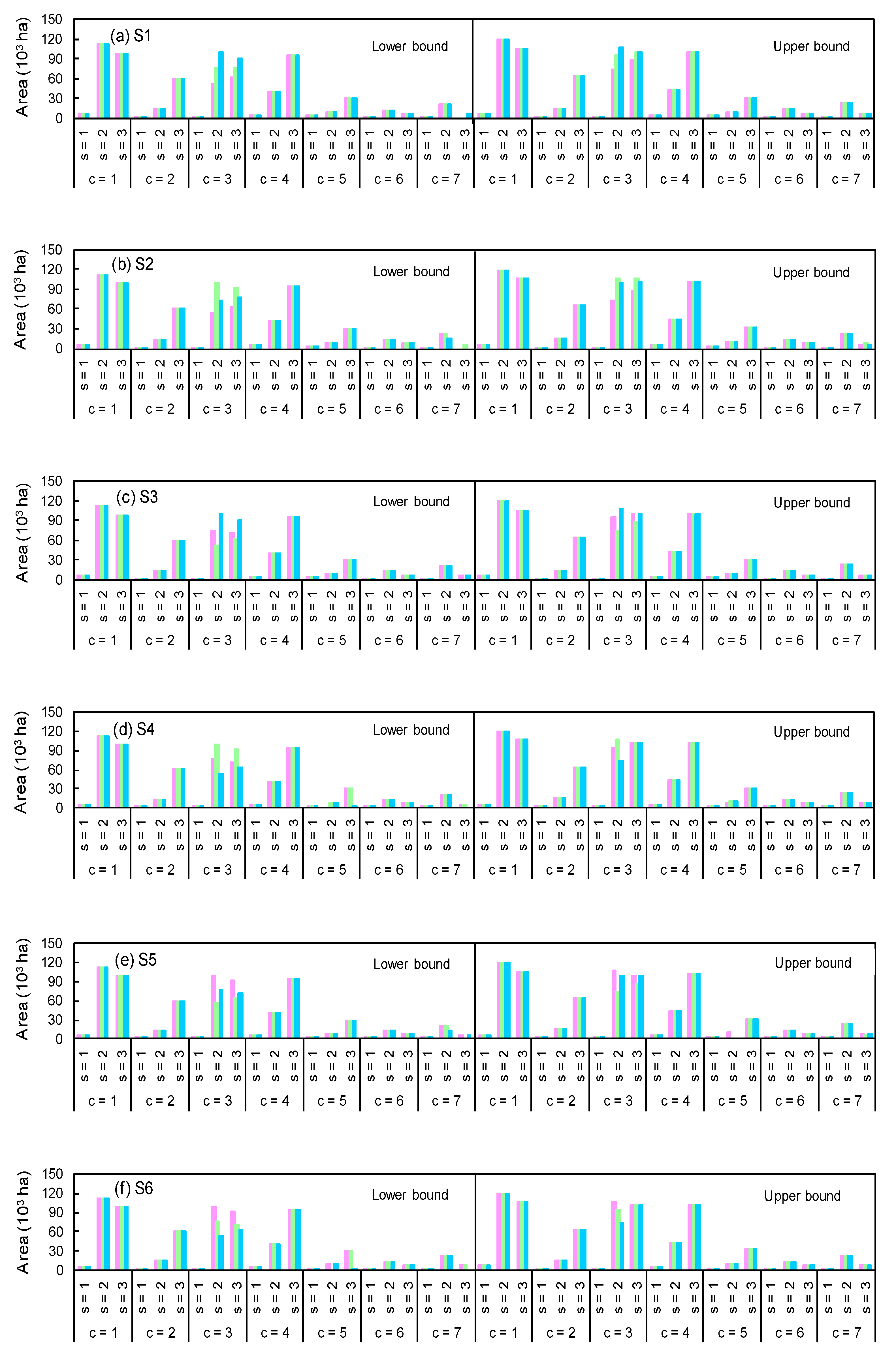
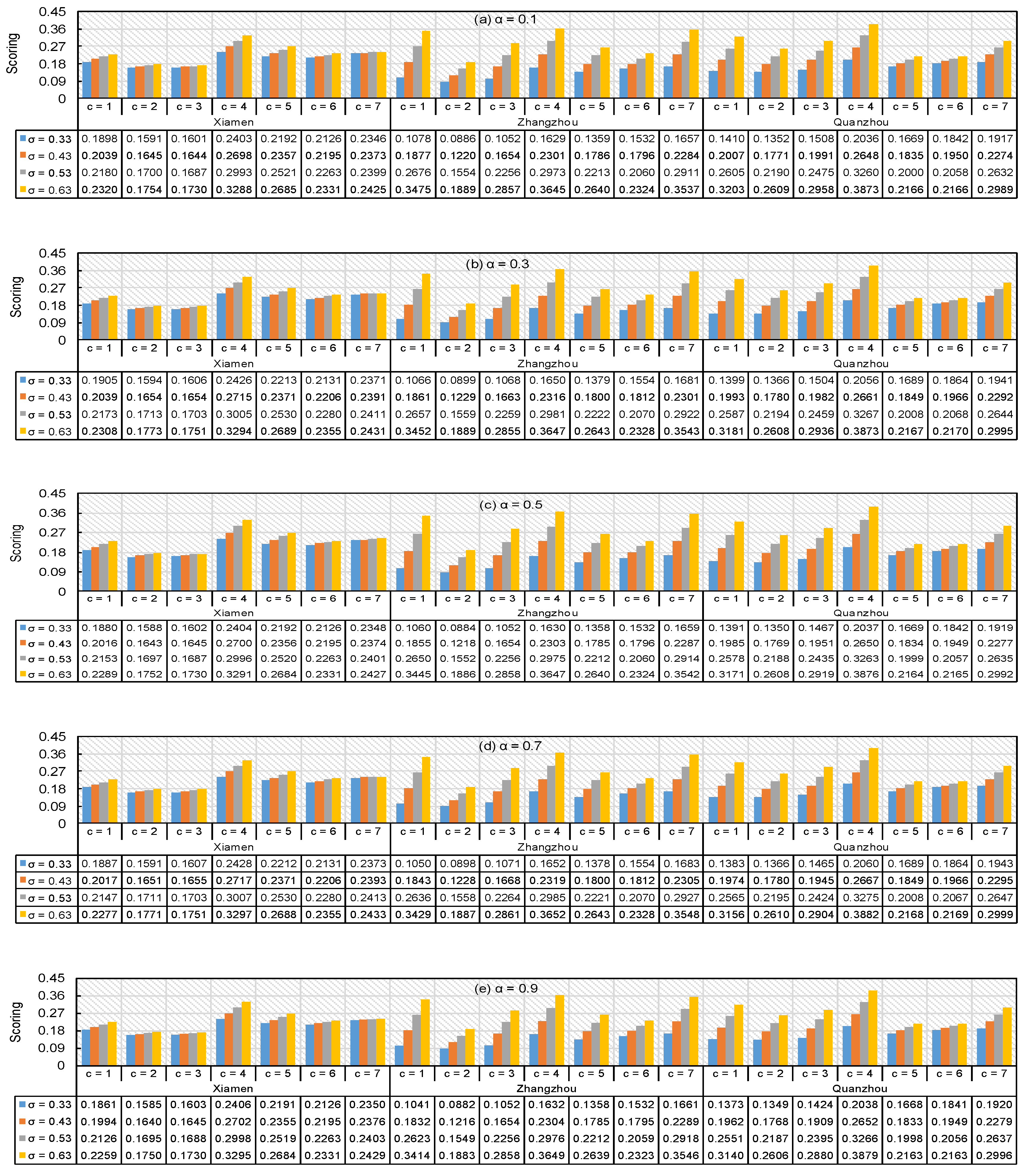
The IF-OWA method was then employed to assess the system security according to decision makers’ optimism degrees. Ten criteria including CY, CA, MP, IQR, CAS, CGS, AD, AG, FA, and PU were selected, which were determined after running the ITSP model.
Table 4 presents the weighting vectors (
) of the 10 criteria under each σ value. Important degrees of criteria are represented as linguistic quantifiers (L for “low”, LM for “low-medium”, M for “medium”, MH for “medium-high”, and H for “High”). The linguistic important degrees of the criteria were converted into their equivalent triangular fuzzy numbers and transferred into crisp normalized values.
Table 5 presents defuzzied linguistic quantifiers (
di), in which the normalized values of five important degrees are 0.1333, 0.2500, 0.5000, 0.7500, and 0.8667. Ten criteria can be handled based on Equation (23) to formulate new inputs. Lower bounds represent optimistic data for positive criteria, while lower bounds represent pessimistic data for negative criteria. For instance, market price of early rice is [2.28, 3.12] Yuan/kg in Xiamen, which means that high market price can lead to high benefit (i.e., optimistic condition). Cost of surface water is [2.32, 1.82] Yuan/m
3 in Xiamen, which denotes that high cost of surface water can result in low benefit (i.e., pessimistic condition). All criteria should be normalized (
) using Equation (6) due to their different units. Five α values (0.1, 0.3, 0.5, 0.7, and 0.9) and four σ values (0.33, 0.43, 0.53, and 0.63) were chosen to evaluate the system security.


