Abstract
River discharge data are critical to elaborating on engineering projects and water resources management. Discharge data must be precise and collected with good temporal resolution. To elaborate on a more accurate database, this paper aims to quantify the uncertainty generated while applying Bayesian inference through the GLUE and DREAM methods. Both methods were used to estimate hydraulic parameters and compare between them with Manning’s equation. Throughout the statistical analysis, the uncertainties in the application of the models are used to determine the parameters of Manning’s roughness coefficient and bed slope. The validation was made via a comparison of the calculated maximum and minimum discharges, and the observed flow available at HidroWeb. In conclusion, both methods estimated the hydraulic parameters well, but a higher relative deviation was seen in the intervals with smaller calculated discharges; DREAM appears to be more accurate than GLUE, once the relative deviation in GLUE became greater.
1. Introduction
Monitoring river discharge is important to the maintenance of the environment and water planning. Such data are necessary to elaborate engineering projects aiming to guarantee water availability to the public, as well as industrial and agricultural supply. This can help prevent natural disasters related to flooding and drought as well as provide fluvial transportation.
The methods usually applied to river discharge determination could be performed directly or indirectly. Direct river discharge estimations employ accurate equipment including the Acoustic Doppler Current Profiler (ADCP), Acoustic Doppler Velocimeter (ADV), mechanical current meters, drones, and others [1]. Even though these ways of measuring the flow can lead to results with high resolution, this equipment is expensive and may require a professional to deal with the situation in the field and during post-processing [2]. There is also physical risk to the professional handling of this equipment during flooding [1,3,4].
Because of these problems, many authors have worked to develop a better way to solve such difficulties using different approaches. Perumal et al. [3,4,5,6,7] used the velocity term through the Muskingum method, while Aricò et al. [2,8] applied a diffusive hydraulic model (DORA’s numerical scheme) using stage water records. Barbetta et al. [9] estimated the uncertainty generated from discharge determination in real-time, and Choo et al. [10,11,12] applied the entropy theory while estimating discharge using superficial velocity.
All of these authors searched for a better relationship between discharge and stage, i.e., the rating curve. However, the rating curve method uses some simplifications that might increase uncertainty. Aricò et al. [2] and Perumal et al. [3] pointed out the lack of data at high stage flow as a major source of uncertainty because it is necessary to extrapolate the rating curve. Another uncertainty source mentioned by the authors is due to the assumption that the cross-section geometry and roughness are constant and do not present modifications over time.
To solve problems related to uncertainty quantification due to physical properties of the channel, we study here a way to estimate the physical parameters of the channel by determining and analyzing the uncertainty in the estimates of the leading hydraulic parameters involved: Manning’s roughness coefficient (n) and bed slope (S0). Therefore, the main goal of this paper is to estimate the hydraulic parameters in parallel with the database available from Portal HidroWeb of the Brazilian Water Agency (ANA).
The approach was applied to two different statistical methods to estimate the parameters of the model. Beven and Benley [13] developed the first method: Generalized Likelihood Uncertainty Estimation (GLUE). It was used for its simplicity, easy application, and extensive use in this kind of problem [14]. Vrugt et al. (2016) developed the latter method: Differential Evolution Adaptive Metropolis (DREAM) [15]. The DREAM method is more refined than GLUE and estimates the posterior probability of the parameters and is recommended for the application of complex multicriteria problems. The DREAM method also provides a Bayesian estimate of the exact uncertainty and shows significant results versus other algorithms due to its minimized systemic deviation [15,16].
2. Materials and Methods
The study area is located on Meia Ponte River (Figure 1) situated in an urban area. The Meia Ponte River is the main natural channel and it is responsible for urban drainage in Goiania City according to SIEG [17]. The river reaches 41.6 km inside the urban perimeter and is important to the public and industrial local water supply. We analyzed the fluviometric data from station 60640000 installed at the river with coordinates 16°36′48.96″ S and 49°16′46.92″ W available at Portal HidroWeb [18]. The parameters were determined considering steady flow assuming Manning’s equation and applying GLUE and DREAM methods.
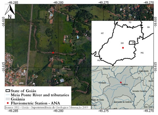
Figure 1.
Meia Ponte River’s and study area.
Parameters estimations were performed for Manning’s roughness (n) dividing it into three parts (n1, n2 e n3) along the cross-section (Figure 2) and to bed slope S0. Initially, it was assigned possible intervals of n3 as 0.1 to 0.3 according to Arcement and Schneider [19]. There is a higher n to flooding areas. To coefficients n1 and n2, were used for possible intervals of 0.02 to 0.2 considering n in natural channels with 30 m or less in width as well as excavated and dredged channels with natural beds; this further considered weathering and the tops with willows [20].
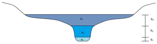
Figure 2.
Representation of n along the cross-section.
Once the possible intervals of n were defined, it was applied to the Manning equation (Equation (1)), the geometry data from the channel, and the stage history (both sets of data from HidroWeb).
Here Qcalc is calculated discharge (m³/s), n is the Manning roughness (s/m1/3), Rh is a hydraulic radius (Equation (2)), Am is flow area (m²), and S0 is the bed slope (m/m).
where Pm is the wetted perimeter.
The geometry parameter values were determined through the bathymetry and the stage hydrograph available from Portal HidroWeb of the Brazilian Water Agency (ANA). The basic data were processed through interpolation to reach a higher number of stage levels to the cross-section area (Figure 3).
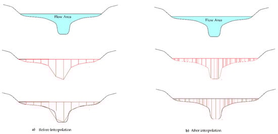
Figure 3.
Scheme showing the cross-section area before (a) and after (b) the trapezoidal interpolation.
The flow area was determined using the trapezoid method (Equation (3)); wetted perimeter was calculated through the sum of distances between the coordinates of the cross-section using Equation (4), as well as applied by [21].
Here, Δz is the number of sections, and N is the number of intervals of the domain; Pm1, Pm2, and Pm3 were calculated using Equation (4).
After defining the flow area and the wetted perimeter, we determined the nneq (equivalent Manning roughness) using Equation (5) according to each case (Table 1).

Table 1.
Definition of each case.
Here, Amt and Rht are, respectively, total wetted area and hydraulic radius; c1, c2, and c3 correspond to each case, as described by Table 1.
2.1. Calibration
To estimate the parameters of the model, we used a three steps process indicated, as usual in a calibration process: (i) objective function definition; (ii) optimization algorithm; and (iii) stop criteria [22]. The objective function is used to point to the development of the analyzed problem in which aim finds those model parameters values that optimize the objective function showing a deviation capable of qualifying the results. The optimization algorithm is a logical procedure to search for the function surface parameters (surface described by the objective function in the space parameters). These parameters optimize (maximize and minimize) the objective function considering the range of values of each parameter. Finally, we applied a stop criterion, which bins the results into the most significant range of estimated parameters, e.g., the convergence of the objective function, the convergence of parameters values, and the maximum number of interactions.
In this work, we applied two different statistical methods to estimate the hydraulic parameters: the GLUE and DREAM methods. This used two distinct objective functions—first, the coefficient of Nash and Sutcliffe [23] (eNS) to GLUE and then, the Sum Squared Error (E) to DREAM.
The stop criteria used were the eNS to GLUE and then the convergence point applying the criterion of Gelman–Rubing (Rest) to DREAM. Both stop criteria used the structure for distinct analysis even though they are similar in some points. They have inclusive methodologies that concomitantly perform the calibration and uncertainty analysis of a model. The uncertainty sources might be summarized, for example, as the estimated parameters of the model, as a model structure, and as observed data [24]. Thus, for both algorithms, the uncertainty analysis is based on the estimated confidence intervals of a dependent variable from an independent variable as expressed in probabilistic terms. The uncertainty analysis in hydrologic fields is an important matter for hydrology. It is closely related to estimate the parameters and validation of the models [25].
2.1.1. GLUE
After determining the intervals of possible parameters (n1, n2, n3, and S0 at Section 2), we consequently found a series of calculated discharge Qcalc (m3/s). By applying the GLUE method, the Qcalc was compared to observed discharge Qobs (m3/s) to determine the Nash–Sutcliffe (eNS) used to determine the representativeness of the estimated parameters (Equation (6)).
Here, eNS is Nash–Sutcliffe [23] that is used to identify mathematically the efficiency of the determination of the discharge Qcalc; Qobs is observed discharge (m3/s); Qcalc is calculated discharge determined by the model (Manning’s equation) using each set of n1, n2, n3, and S0; and Qobsm is the average observed discharge (m3/s).
The parameters were organized in sets to apply the GLUE method. In this case, each set was composed of distinct values of n1, n2, n3 and S0 inside the interval previously determined. The number of sets used in this work was determined through tests. We analyzed four different sizes of sets (NS) and tested NS equal to 100, 1000, 10,000, and 100,000. Moriasi et al. [26] showed that eNS = 0.76 is considered good, but, in this paper, eNS was deemed to be acceptable above 0.9 to get a more representative estimate of the parameters. Another criterion used to choose NS was the time of computing spent to get enough sets above 0.9.
2.1.2. DREAM
The DREAM method uses a series of interactions to find the studied parameters similar to GLUE. However, the method works through the scheme of Markov Chain Monte Carlo (MCMC) where, following the steps defined by Vrugt [15], the number of parameters to be studied was first established, i.e., the terms n1, n2, n3, and S0 (in this case, 4 parameters) following the possible intervals previously defined. The second step was to determine the size of the population followed by the third step—determine the length of the subpopulation to be studied at a time, i.e., 40,000 and 100. The fourth step was to determine the representativeness of the results (Equation (7)), and then the fifth step selects the first 80% higher values and develops the fourth and fifth steps (MCMC) until it reaches the stopping criterion of Gelman Rubin [27], in which the convergence is determined when Rest is under 1.2.
Here, E(θ) is the error value to subpopulation analyzed (θ); NI is the order in which the subpopulations are rated; σ(t) is the observed variable and; σ(t|θ) is the calculated value of the variable using the subpopulation posterior θ.
This method initially applies different sets of θ at the same time assigning n1, n2, n3, and S0. The subpopulations analyzed θ are globally compared to each other in order to gather the most representative solutions to each θ. In other words, the method can select the most representative parameters of n1, n2, n3, and S0 and create new subpopulations to re-route again until this narrows to the best sets of n1, n2, n3, and S0 observing the convergence point of Gelman and Rubin [27] Rest < 1.2.
2.2. Validation and Uncertainty Quantification
The aim of the validation is to analyze if the implemented calibration process can generate results next to the reality. This includes how representative the estimation is and the efficiency of the model [28].
After determining the parameters, we next calculated the Qcalc maximum and minimum with both GLUE and DREAM via Manning’s equation. We assigned the estimated parameters (n1, n2, n3, and S0) and the stage water. Then, the Qcalc maximum and minimum were compared to its respective discharge observed Qobs both from 2017, as well as the data used in the calibration process, available from Portal HidroWeb [18]. The Qcalc maximum and minimum were restricted to its values above 5% of the minimum discharge and 95% under the maximum discharge.
The maximum and minimum discharge were first applied to validate the estimated parameters and to make a brief analysis of uncertainty. According to Pereira [16], the validation of the model consists of reapplying the estimated parameters (in new simulations) with new input data in the same model. Pereira reported that it is necessary to reach new results while developing new simulations compared to the previous simulation performed in the parameters estimation step to validate the method. Here, graphics were elaborated to compare Qcalc and Qobs and to then determine the deviation through them. For this validation, we analyzed the representativeness of the parameters while being applied to determine Qcalc and posterior comparison to Qobs.
After the validation step, the graphics pointed to historical series comprehended in 2007 to 2016, highlighting three different discharges peaks in each year while first analyzing events with higher discharge. This then moved to intermediary discharge flow and finally to lower discharge in drought seasons.
3. Results and Discussion
The results of this paper are divided into three parts. The first one presents the results for GLUE, and the second one is for DREAM. The final discussion compares the two methods and applies their estimated parameters.
3.1. GLUE
After identifying the number of sets, NS was determined as equal to 100,000 because this number of sets had 1564 sets with eNS above 0.90; the computing time was 4 h and 15 min—a time that is considered acceptable when compared with others realized tests and their NS with eNS above 0.90 (Table 2).
Table 2.
Results for the definition of NS.
When considering the set size (NS) equal to 100 (Table 2), there were no parameter sets with eNS above 0.90. The computing time was ignored due to the non-compliance of the first requirement. For NS equal 1000, there were only two sets above the adopted minimum eNS, and these were also discarded regardless of their computing time. NS equal to 10,000 found 38 sets, which is a reasonable quantity but yet without the representability required. Finally, NS equal to 100,000 found 1564 sets with eNS above 0.90 and a computing time a bit superior to 4 h and 15 min. This was a machine with AMD Ryzen 7 1800X Eight-Core processor with 72 GFLOPS.
The GLUE method used the observed discharge obtained from HidroWeb. We then applied the rating curve method while the calculated discharge was estimated through Manning’s equation. We also previously determined the uncertainty range for n1 (0.02 to 0.2), n2 (0.02 to 0.2), n3 (0.1 to 0.3), and S0 (10−5 to 10−1). This uncertainty range was restricted to n1 (0.041 to 0.2), n2 (0.02 to 0.2), n3 (0.1 to 0.3), and S0 (4 × 10⁻⁴ to 10−2) after estimations and classifications of the capacity of the parameters to represent the observed value; the Nash–Sutcliffe coefficient was higher than 0.9.
To compare between the discharge from ANA’s database and the calculated discharge, we next elaborated a boxplot to show the difference between rating curve discharge (presented as observed discharge) and the calculated discharge applying the estimated parameters into Manning’s equation. Figure 4 presents the deviation between the observed and calculated discharges while applying the hydraulic parameters estimated through the GLUE method where the absolute deviation was between 1.26 and 3.33 m³/s when ruling out all the outlier results.
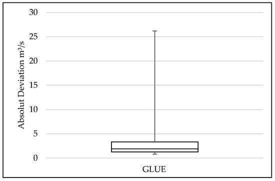
Figure 4.
Boxplot of absolute deviation, point the outlier results—GLUE.
In addition to absolute deviation, we also applied the relative deviation results in to a boxplot graph to exclude the outliers. The Figure 5 demonstrates that the relative deviation actually remained between 8.03 and 15.10%.
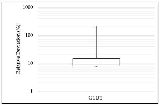
Figure 5.
Boxplot of relative deviation (logarithmical scale)—GLUE.
Figure 6 presents the observed discharges being compared to the interval of calculated discharges. The observed discharge remained between the range of maximum and minimum calculated discharges for the water level in the normal flow and overflow cases. For water levels less than 1.5 m, the observed flows were lower than the minimum calculated discharges that were outside the expected range. This can be related to possible changes downstream that alter the boundary condition. This is a difficulty of the model to adjust to the lower measurements.
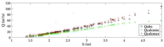
Figure 6.
Interval of calculated and observed discharges—GLUE.
Figure 6 shows that the adjustments of the parameters were satisfactory once the calculated discharges presented a similar trend to the observed discharges when analyzing the behavior of the discharge in relation to the water level.
To show how the estimated parameter can affect the discharge determination, a graph of matrices was prepared (Figure 7), values above the main diagonal are the correlations between the estimated parameters.
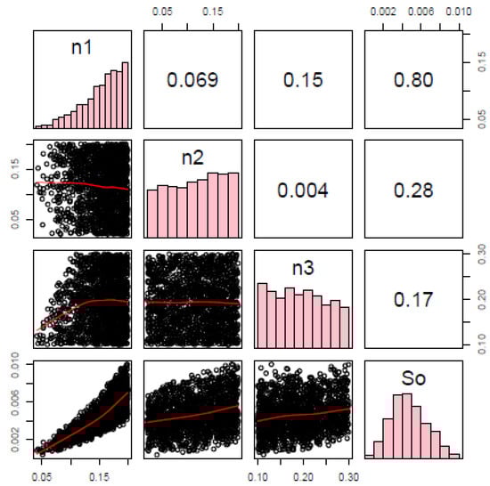
Figure 7.
Matrix of graphics relating n1, n2, n3, and S0—GLUE. The main diagonal shows the histogram of each parameter demonstrating the frequency with each value of n1, n2, n3, and S0 in the distribution. Below the main diagonal, we see the scatter plots for each pair of parameters. The line is drawn to guide the eye.
Figure 7 also points to the relationship between the parameters n1, n2, and n3 presenting a low correlation where the highest was 0.15. This may lead to the conclusion that the parameters of Manning roughness coefficient, when correlated with each other, do not present a similar distribution. The parameters n1, n2, and n3 were compared individually with declivity of the channel S0. There was higher correlation between the parameters n1 and S0 of + 0.80, which indicates a strong relationship where the variables move relatively together. This may have occurred because the value of the stage was usually below 1.5 m where only the roughness coefficient n1 is considered. The values of n1 were rising indicating that a higher n1 value has a higher number of individuals while n2 and n3 showed that the number of individuals were relatively constant over their distribution. The distribution of the values of S0 show that the lowest and highest values presented a lower number of accepted individuals. The values of S0 were concentrated close to the median of the interval of the selected data. Scatter plot analysis shows that the relationship between n1 and S0 reaffirms the strong correlation between them. The values are distributed very close to each other, which is not seen in other relations.
Once we validated these parameters, we next elaborated the graphics to determine the uncertainty range from 2007 to 2016. In drought seasons with low observed discharges, the uncertainty range stayed below the minimum calculated discharges, i.e., outside the uncertainty range. On the other hand, during flooding seasons, the observed discharges stayed inside the uncertainty range as seen in Figure 8 with data from 2016 as an example.
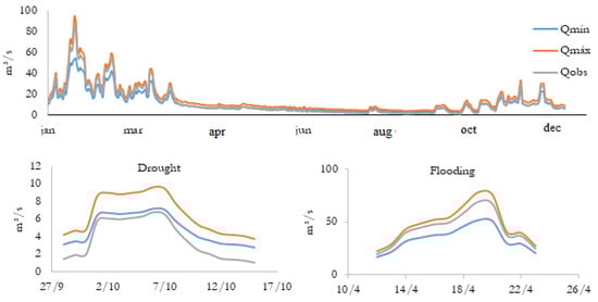
Figure 8.
Annual discharge of 2016—GLUE.
Figure 8 shows that the values of the rating curve’s discharges are lower than the minimum calculated discharges. This starts from the discharge of 6.17 m³/s and continues to through all of the drought season or while the value of discharge is below 6.17 m³/s.
Figure 9 shows that the highest relative deviation was about 92.08% in 2009, while the lowest occurred in 2016 with 48.75%. The year 2016 presented the greatest variation in its relative deviation between 48.75 to 90.75%.
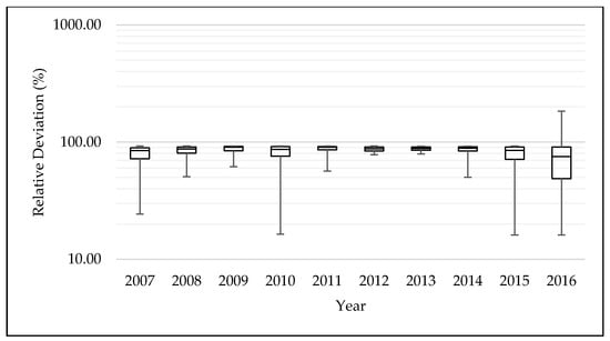
Figure 9.
Relative deviation of 2007 to 2016—GLUE.
3.2. DREAM
The values of absolute and relative deviation were also created via the DREAM method (Figure 10 and Figure 11, respectively). The absolute deviation found through the GLUE method was between 0.59 and 2.09 m³/s when ruled out all the outlier results (Figure 10).
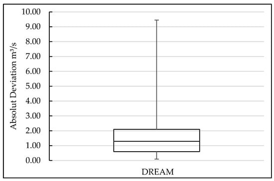
Figure 10.
Boxplot of absolute deviation—DREAM.
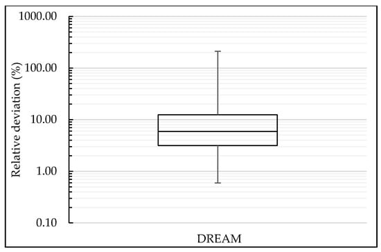
Figure 11.
Boxplot of relative deviation (logarithmical scale) and points on the outlier results—GLUE.
In addition to absolute deviation, we also applied the relative deviation results into a boxplot graphic to rule out all the outliers and narrow the average results. Figure 11 demonstrates that the relative deviation is between 3.16% and 12.40%. This is exactly as happened in the calibration with the GLUE method: the relative deviation found via DREAM at a lower hydrographic stage is greater than compared to higher water levels.
The observed discharges stayed mostly very close to the interval of maximum and minimum calculated discharges. They show a well-defined behavior with minimum distance from themselves (Figure 12).
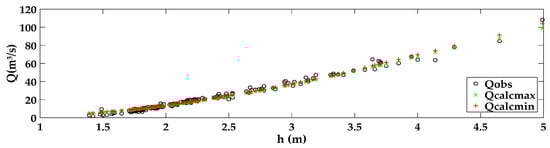
Figure 12.
Interval of calculated and observed discharges—DREAM.
Figure 13 presents the relation between the estimated DREAM parameters. These include the superior part of the main diagonal. The values of correlations between each parameter where the correlation between n1 and S0 present the highest value of 0.99. That means that n1 and S0 have a strong correlation with each other, and, consequently, presents a well-defined distribution between them. For the correlations of the other parameters of the Manning roughness coefficient versus S0, there were strong correlations between the parameters n3 × S0 (0.91): the correlation between n2 × S0 was only 0.014.
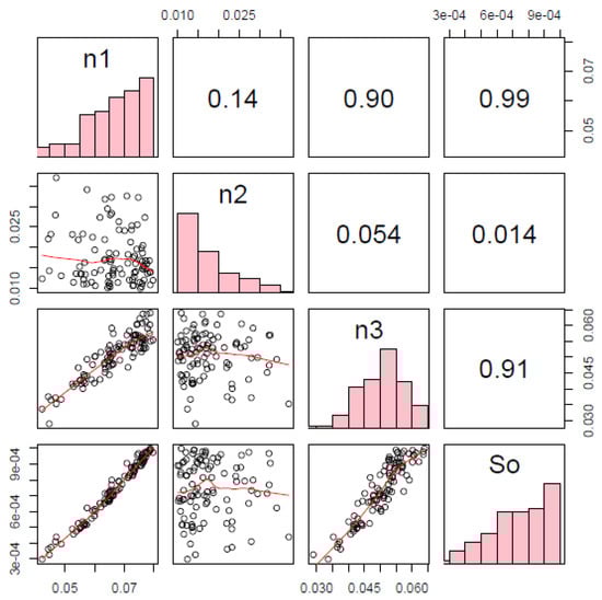
Figure 13.
Matrix of graphics relating n1, n2, n3 and S0—DREAM.
The frequency histogram of each parameter was seen on the main diagonal of the matrix (Figure 13). For n1, a higher number of individuals were seen as the ones of higher values while for n2 the higher frequency was the same as those with the necessary lowest Manning roughness coefficient. In addition, n3 had a higher number of individuals that stayed very close to the median of the interval. For S0, the highest values of declivity present higher numbers of individuals. Below the main diagonal of the matrix, there were dispersion graphics that agree with the values of correlations n1 and S0. These results showed a well-defined distribution between each other as well as n2 × S0; however, the dots were presented distributed very far from each other for n3 × S0.
After the validation of the parameters, we next determined the calculated discharges for the years of 2007 to 2016. Figure 14 presents the interval of uncertainties generated by the calculated discharge, as well as the observed discharges to the year of 2014. Figure 14 presents the annual discharge including drought and flooding season discharges. While some dots of observed discharge have stayed outside of the uncertainty interval, in general, the results were satisfactory and simulated the discharges data quite similar to real results.
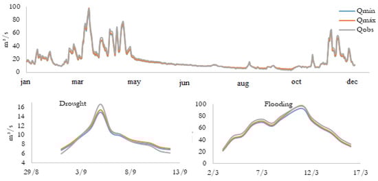
Figure 14.
Annual discharge of 2014—DREAM.
Figure 15 shows that the highest relative deviation was recorded in 2016. It is 54%, while the lowest was in 2009 with 2.04%. Even though 54% was found as the highest relative deviation, it might be important to highlight that, versus the other years analyzed, 2015 was the worst case: the values were between 20 and 6.71%.
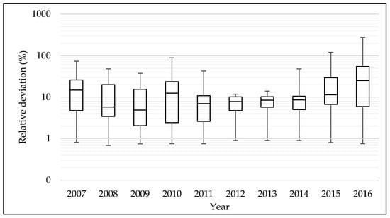
Figure 15.
Relative deviation trough 2007 to 2016—GLUE.
3.3. Discussion
Both methodologies presented valid parameters where the maximum and minimum calculated average discharges presented similar behavior of the observed discharges. However, before beginning any more detailed comparison, we note that GLUE presents a less complex methodology than DREAM. Even though the input data is the same, DREAM uses a Bayesian base of a formal character and can present more restricted intervals of uncertainty.
The deviation found in the GLUE reaches a little more than 92% while it was 54% in DREAM. In general, the maximum and minimum deviation generated through the application of GLUE were above the ones found on DREAM especially 2016 when the highest maximum deviation occurred in both cases: 92% and 54% for GLUE and DREAM, respectively. This is similar to Thi, Ball, and Dao [29].
The calibration applying to the GLUE method showed considerable results (not only because of the results, but also due to its easily application); however, we considered DREAM to show better results when compared to GLUE. The DREAM method kept its deviation below 54% in its worst-case and below 20% for most the analyzed period of 2007 to 2016.
The GLUE method still presents a higher absolute deviation on the discharge peaks as in cases where the height stayed above 4 m. When validating the calculated discharges, we note values of observed discharges outside the interval of calculated discharges. This result was expected because of extreme events that usually presents a higher uncertain degree [30].
Both methods show a strong relationship between observed and calculated discharge. Both methods show that the relative deviation and the flow have an inverse relationship with the higher discharge showing the smallest relative deviations. Therefore, in this case, the simulated lowest discharges seemed to overestimate the observed discharges.
When comparing both methods, the parameters estimated by DREAM presented a higher relation between them versus GLUE parameters (in Figure 9 and Figure 15). Another factor to be considered is the time of data processing of both methods. GLUE took 4.5 h to generate and analyze 100,000 sets with four parameters each leading to a little more than 1500 satisfactory sets. In contrast, DREAM took 30 min to generate and analyze 40,000 sets while selecting only 100 sets. These were determined to be more accurate than the ones found via GLUE.
4. Conclusions
The determination of n1, n2, n3, and S0 parameters presented satisfactory results for the stage inside the height interval denominated normal flow stage via both methods but with some relative deviation above 50%. This might be justified by the occurrence of random deviation: reading deviation given by the data provided by HidroWeb, as well as by systematic deviation including for the case of simplification determining the river channel as being constant and without alteration over time. Both sources of the uncertainty affect the rating curve and bathymetry of the cross-section that are the main input data for both methods.
The GLUE method generated sets of parameters in a way that the calculated discharges were overestimated. This fact can be better observed in drought seasons when the values of stages were inferior; the respective observed discharges are lower than the minimum calculated discharges. To summarize, the model simulates better on flooding seasons or while there is flow on the normal flow stage. The same may be said of DREAM, where the overestimation was smaller. Keeping the values of calculated discharges close to the observed leads to good result for all stages.
Because of the uncertainty generated through the rating-curve and bathymetry from HidroWeb, it might be recommended to monitor the stage over one year and redo the bathymetry with higher frequency. Updating the bathymetry of the cross-section to be used in the model might minimize the random deviation of the readings that may have occurred in the field.
Author Contributions
G.d.C.d.R. wrote the paper and analyzed the data; G.S.F., T.S.R.P. and K.T.M.F. revised the manuscript; G.d.C.d.R. and K.T.M.F. contributed to research development; K.T.M.F. managed the research and development projects. All authors have read and agreed to the published version of the manuscript.
Funding
This study was financed in part by the Coordenação de Aperfeiçoamento de Pessoal de Nível Superior – Brasil (CAPES), grant number 52001016102P4, and financial support by Financiadora de Estudos e Projetos (Finep). The authors thank the support of laboratory of Hydraulics of UFG, and to Tomas Rosa Simões for their technical support in the fieldwork.
Conflicts of Interest
The authors declare no conflict of interest.
References
- De Oliveira, F.A.; Pereira, T.S.R.; Soares, A.K.; Formiga, K.T.M. Uso de modelo hidrodinâmico para determinação da vazão a partir de medições de nível. Rev. Bras. Recur. Hídricos 2016, 21, 707–718. [Google Scholar] [CrossRef][Green Version]
- Aricò, C.; Nasello, C.; Tucciarelli, T. Using unsteady-state water level data to estimate channel roughness and discharge hydrograph. Adv. Water Resour. 2009, 32, 1223–1240. [Google Scholar] [CrossRef]
- Perumal, M.; Moramarco, T.; Sahoo, B.; Barbetta, S. A methodology for discharge estimation and rating curve development at ungauged river sites. Water Resour. Res. 2007, 43, 02412. [Google Scholar] [CrossRef]
- Perumal, M.; Moramarco, T.; Sahoo, B.; Barbetta, S. On the practical applicability of the VPMS routing method for rating curve development at ungauged river sites. Water Resour. Res. 2010, 46. [Google Scholar] [CrossRef]
- Perumal, M. Hydrodynamic derivation of a variable parameter Muskingum method: 2. Verification. Hydrol. Sci. J. 1994, 39, 443–458. [Google Scholar] [CrossRef]
- Perumal, M.; Price, R.K. A fully mass conservative variable parameter McCarthy–Muskingum method: Theory and verification. J. Hydrol. 2013, 502, 89–102. [Google Scholar] [CrossRef]
- Perumal, M.; Sahoo, B.; Moramarco, T.; Barbetta, S. Multilinear Muskingum Method for Stage-Hydrograph Routing in Compound Channels. J. Hydrol. Eng. 2009, 14, 663–670. [Google Scholar] [CrossRef]
- Aricò, C.; Corato, G.; Tucciarelli, T.; Ben Meftah, M.; Petrillo, A.F.; Mossa, M. Discharge estimation in open channels by means of water level hydrograph analysis. J. Hydraul. Res. 2010, 48, 612–619. [Google Scholar] [CrossRef]
- Barbetta, S.; Brocca, L.; Melone, F.; Moramarco, T.; Singh, V.P. Addressing the Uncertainty Assessment for Real-Time Stage Forecasting. World Environ. Water Resour. Congr. 2011, 4791–4800. [Google Scholar] [CrossRef]
- Choo, T.H.; Chae, S.K.; Yoon, H.C.; Choo, Y.M. Discharge prediction using hydraulic characteristics of mean velocity equation. Environ. Earth Sci. 2014, 71, 675–683. [Google Scholar] [CrossRef]
- Choo, T.H.; Hong, S.H.; Yoon, H.C.; Yun, G.S.; Chae, S.K. The estimation of discharge in unsteady flow conditions, showing a characteristic loop form. Environ. Earth Sci. 2015, 73, 4451–4460. [Google Scholar] [CrossRef]
- Choo, T.H.; Yoon, H.C.; Lee, S.J. An estimation of discharge using mean velocity derived through Chiu’s velocity equation. Environ. Earth Sci. 2013, 69, 247–256. [Google Scholar] [CrossRef]
- Beven, K.J.; Binley, A.M. The future of distributed models: Model calibration and uncertainty prediction. Hydrol. Process. 1992, 6, 279–298. [Google Scholar] [CrossRef]
- Vrugt, J.A.; Ter Braak, C.J.F. DREAM(D): An adaptive Markov Chain Monte Carlo simulation algorithm to solve discrete, noncontinuous, and combinatorial posterior parameter estimation problems. Hydrol. Earth Syst. Sci. 2011, 15, 3701–3713. [Google Scholar] [CrossRef]
- Vrugt, J.A. Markov chain Monte Carlo simulation using the DREAM software package: Theory, concepts, and MATLAB implementation. Environ. Model. Softw. 2016, 75, 273–316. [Google Scholar] [CrossRef]
- PEREIRA, T.S.R. Modelagem e Monitoramento Hidrológico Das Bacias Hidrográficas Dos Córregos Botafogo e Cascavel, Goiânia—Go. Master’s Thesis, Universidade Federal de Goias, Goiania, Brazil, 2015. [Google Scholar]
- SIEG. Sistema de Informações Geográficas do Estado de Goiás. Secretaria de Estado de Gestão e Planejamento—SEGPLAN 2017. Available online: http://www.sieg.go.gov.br/siegdownloads/ (accessed on 1 November 2019).
- Portal HidroWeb. Agência Nacional de Água. Available online: https://www.snirh.gov.br/hidroweb/publico/apresentacao.jsf (accessed on 30 October 2018).
- Arcement, G.J.; Schneider, V.R. Guide for selecting Manning’s roughness coefficients for natural channels and flood plains. U.S. Geol. Surv. Water-Supply Pap. 1989, 2339, 38. [Google Scholar] [CrossRef]
- CHOW, V.T. Open Channel Hydraulics; McGraw-Hill: New York, NY, USA, 1959; 680p. [Google Scholar]
- Pan, F.; Wang, C.; Xi, X. Constructing river stage-discharge rating curves using remotely sensed river cross-sectional inundation areas and river bathymetry. J. Hydrol. 2016, 540, 670–687. [Google Scholar] [CrossRef]
- Bravo, J.M.; Piccilli, D.G.A.; Collischonn, W.; Tassi, R.; Meller, A.; Tucci, C.E.M. Avaliação visual e numérica da calibração do modelo hidrológico IPH II com fins educacionais. In XVII Simpósio Brasileiro de Recursos Hídricos; ABRH: São Paulo, Brazil, 2007; pp. 1–20. [Google Scholar]
- Nash, J.; Sutcliffe, J. River flow forecasting through conceptual models part I—A discussion of principles. J. Hydrol. 1970, 10, 282–290. [Google Scholar] [CrossRef]
- Chow, V.T.; Maidment, D.R.; Mays, L.W. Applied Hydrology; Series in Water Resources Environmental Engineering; McGraw-Hill: New York, NY, USA, 1988. [Google Scholar]
- Montanari, A. Uncertainty of Hydrological Predictions. In Treatise on Water Science; PETER, W., Ed.; Elsevier: Oxford, UK, 2011; pp. 459–478. [Google Scholar]
- Moriasi, D.N.; Arnold, J.G.; Van Liew, M.W.; Bingner, R.L.; Harmel, R.D.; Veith, T.L. Model Evaluation Guidelines for Systematic Quantification of Accuracy in Watershed Simulations. Trans. ASABE 2007, 50, 885–900. [Google Scholar] [CrossRef]
- Gelman, A.G.; Rubin, D.B. Inference from iterative simulation using multiple sequences. Stat. Sci. 1992, 7, 457–472. [Google Scholar] [CrossRef]
- Seibt, A.C. Modelagem Hidrológica da Bacia Hidrográfica do Córrego Botafogo—Goiânia, GO. Dissertação (Mestrado). Programa de Pós-Graduação em Engenharia do Meio Ambiente. Master’s Thesis, Universidade Federal de Goiás, Goiânia, Brazil, 2013. [Google Scholar]
- Cu Thi, P.; Ball, J.E.; Dao, N.H. Uncertainty Estimation Using the Glue and Bayesian Approaches in Flood Estimation: A case Study—Ba River, Vietnam. Water 2018, 10, 1641. [Google Scholar] [CrossRef]
- Di Baldassarre, G.; Montanari, A. Uncertainty in river discharge observations: A quantitative analysis. Hydrol. Earth Syst. Sci. 2009, 13, 39–61. [Google Scholar] [CrossRef]


Publisher’s Note: MDPI stays neutral with regard to jurisdictional claims in published maps and institutional affiliations. |
© 2020 by the authors. Licensee MDPI, Basel, Switzerland. This article is an open access article distributed under the terms and conditions of the Creative Commons Attribution (CC BY) license (http://creativecommons.org/licenses/by/4.0/).