Gap-Filling of Surface Fluxes Using Machine Learning Algorithms in Various Ecosystems


Abstract
:1. Introduction
2. Study Sites and Data
2.1. Grassland
2.2. Rice Paddy Field
2.3. Forest
3. Methods
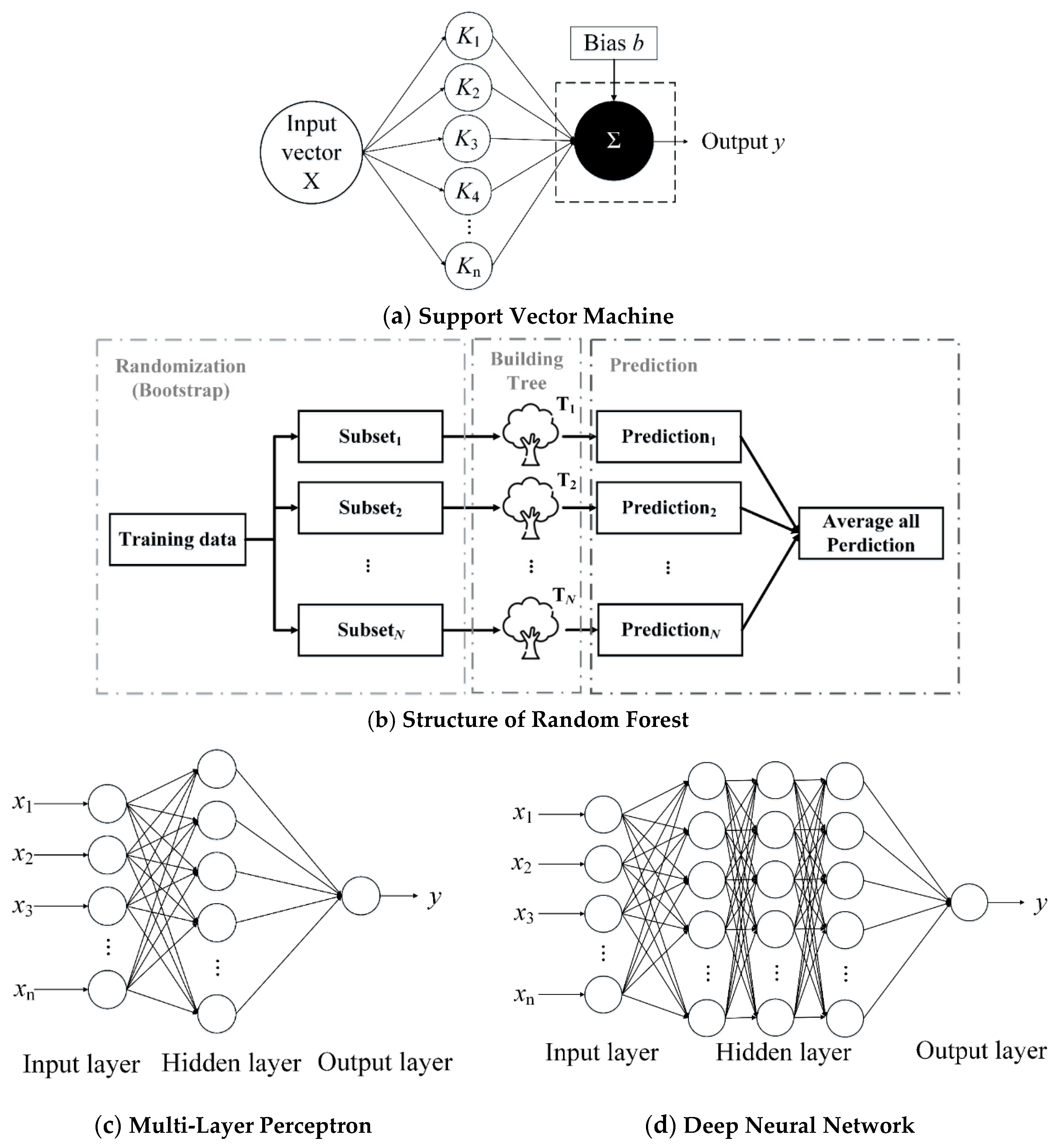
3.1. Machine Learning Algorithms
3.1.1. Support Vector Machine (SVM)
3.1.2. Random Forest (RF)
3.1.3. Multi-Layer Perceptron (MLP)
3.1.4. Deep Neural Network (DNN)
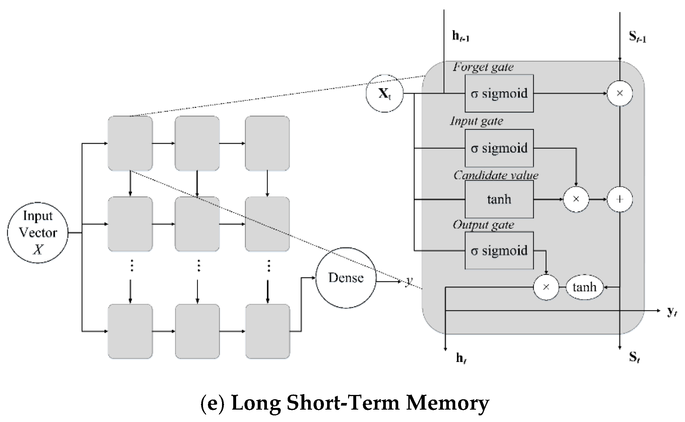
3.1.5. Long Short-Term Memory (LSTM)
3.1.6. Input Variables for Training the ML Models
3.2. Penman–Monteith Equation
3.3. Flux Gap Scenario
3.4. Research Process and Performance Metrics
3.4.1. Research Process
- (1)
- Explore the optimal combinations of input variables for constructing the five ML models for gap-filling of surface fluxes at the three sites, and then compare the model performance. For constructing the ML model, the ratio of data sets for training, validation, and testing was 5:3:2, and each of the data sets was randomly selected with uniform distribution.
- (2)
- In the second stage, the best ML model selected from the first stage was compared with the P–M equation to explore the water vapor flux gap-filling accuracy of both methods at the three ecosystems. The determination of rst for the P–M equation at the three sites is described in Appendix B.
- (3)
- In the third stage, the relation between gap length (one hour, half day, one day, and one week) and training data length (20 to 1600 h) was investigated by the steps in Section 3.3. The ML model adopted here was the best model selected from the first stage.
3.4.2. Performance Metrics
- (1)
- Root mean square error (RMSE)where and are the values from observation and model prediction, respectively, and n represents the total number of data points.
- (2)
- Mean absolute error (MAE)
- (3)
- Coefficient of determination (R2)where is the mean of the observed values and represents the mean of the estimated values.
- (4)
- Coefficient of efficiency (CE)
4. Results and Discussion
4.1. Optimal Input Combinations for Training ML Models
- (1)
- For the grassland, the improvements by including time factors in the input combination are less than 5% for all three fluxes. For the rice paddy field, the improvements for RMSE for the three fluxes range from 8.6 to 19.7%, showing that time factors’ influence is larger at this site. For the forest, this influence on CO2 flux is small (2.9%), but it is larger for water vapor and sensible heat fluxes (7.26–7.9%, respectively).
- (2)
- Concerning the hysteresis factors, at the grassland site, these factors have no influence on all three fluxes. For the rice paddy, the influence on CO2 flux is less important, but important for water vapor and sensible heat fluxes (RMSE improved by 8.72–9.50%). For the forest site, the influence on CO2 flux is important (RMSE improved by 8.10%), but the influence on both LE and H is small (improvement rates of RMSE both less than 2%). Cui et al. [37] found that the magnitude of hysteresis between LE and net radiation is large on water surfaces and small on land surfaces. Our results for LE reveal that the hysteresis factors are stronger for the rice paddy field (flooded with water during growing season), but small for forest and grassland sites. This is consistent with the finding of Cui et al. [37].
4.2. Comparisons of Gap-Filling by ML Models
4.2.1. Carbon Dioxide Flux
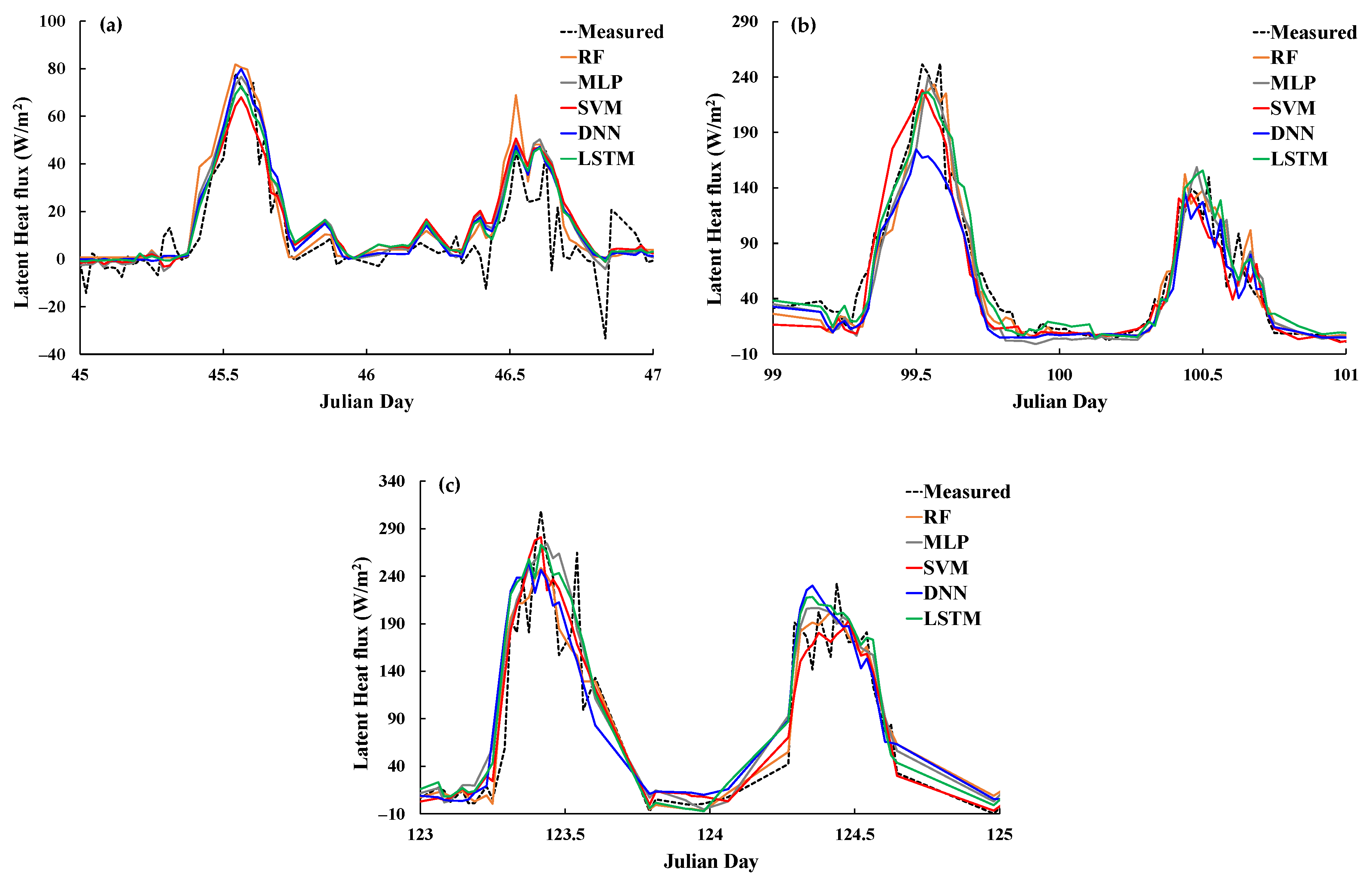
4.2.2. Latent Heat Flux
4.2.3. Sensible Heat Flux
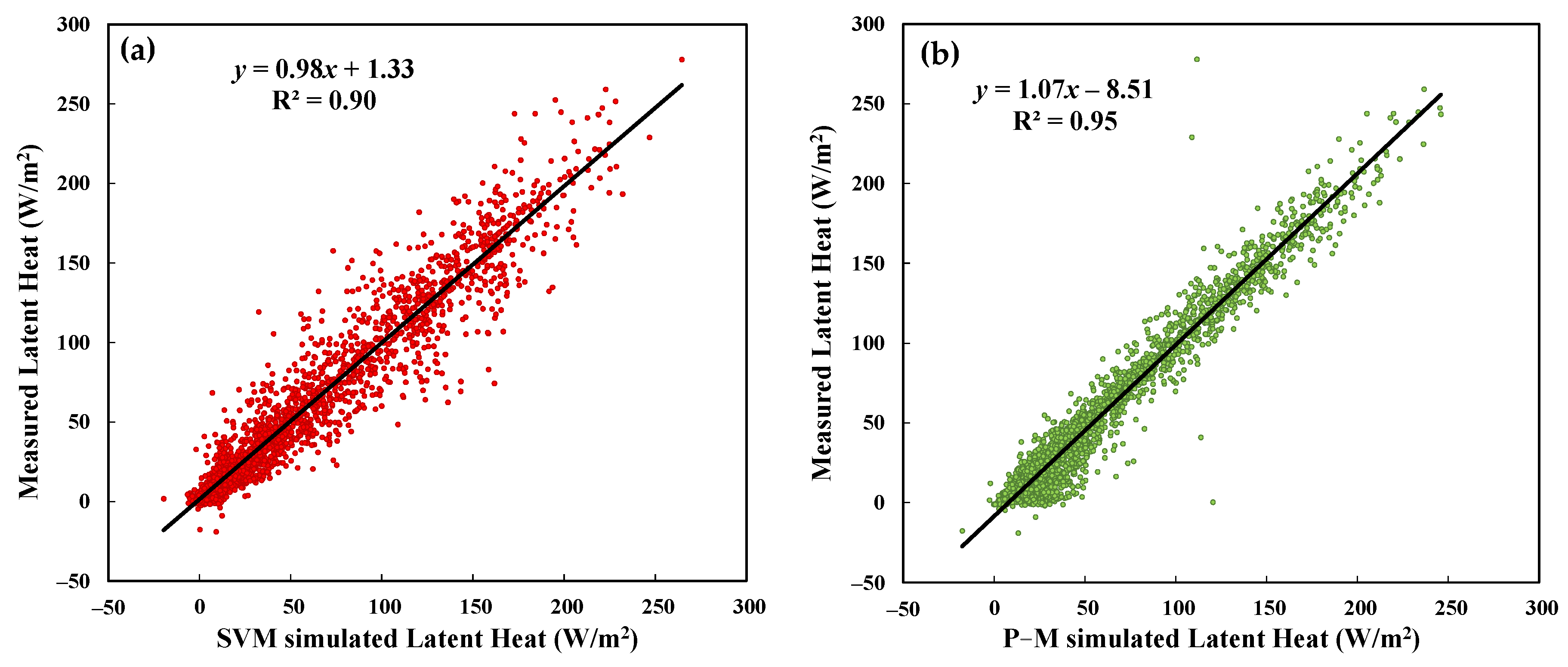
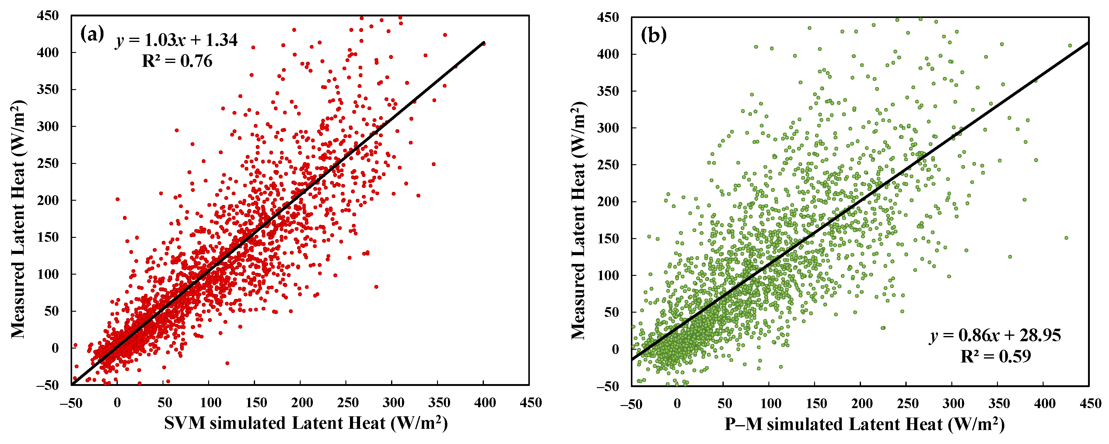
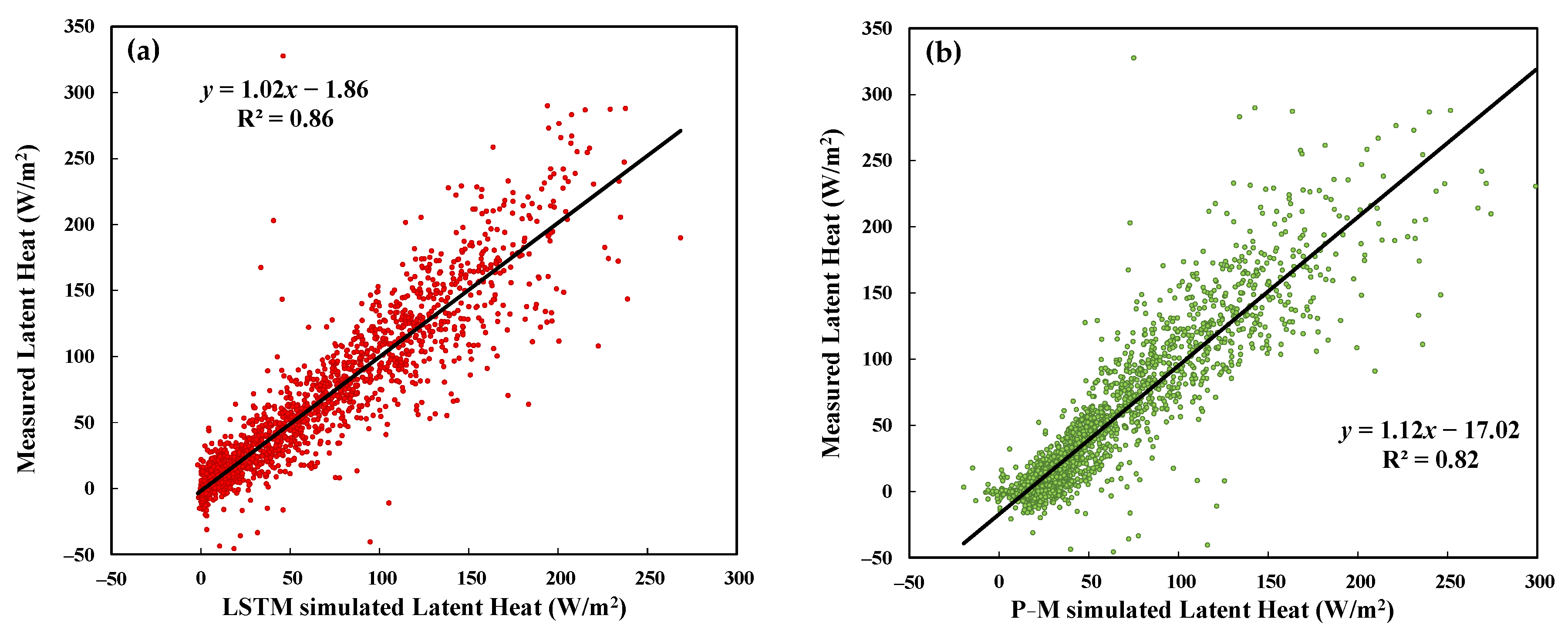
4.3. Comparison between Machine Learning Model and Penman–Monteith Equation
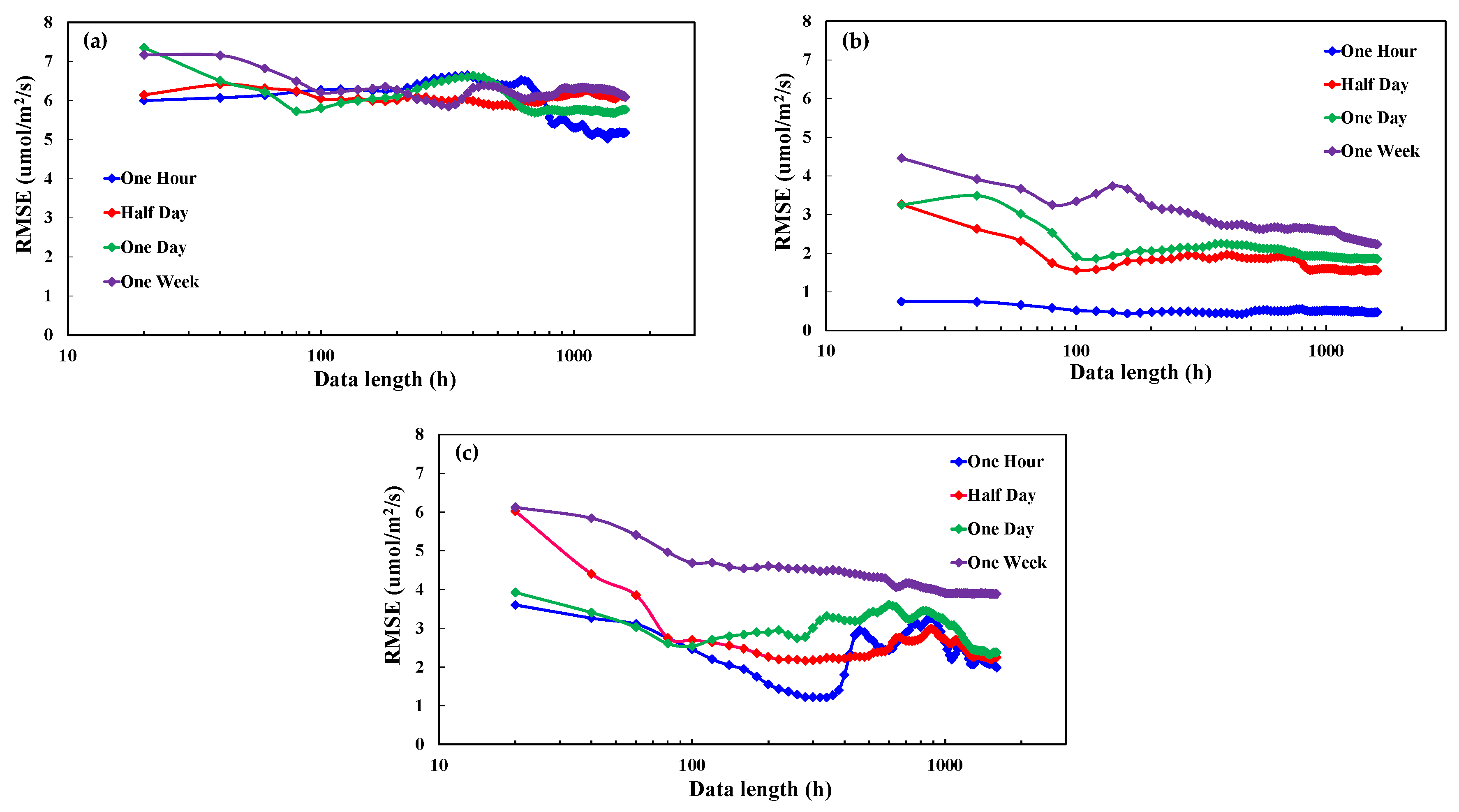
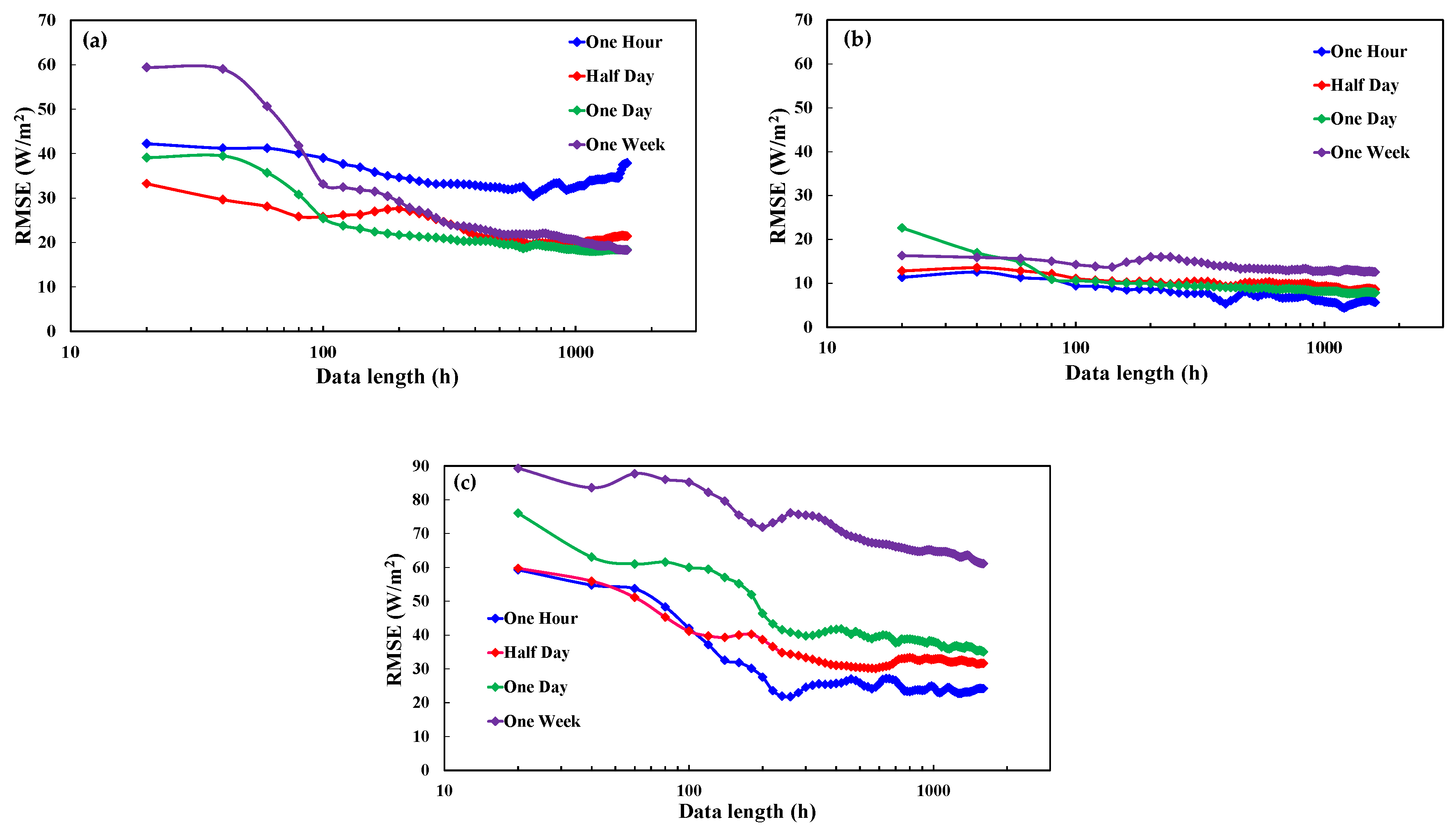
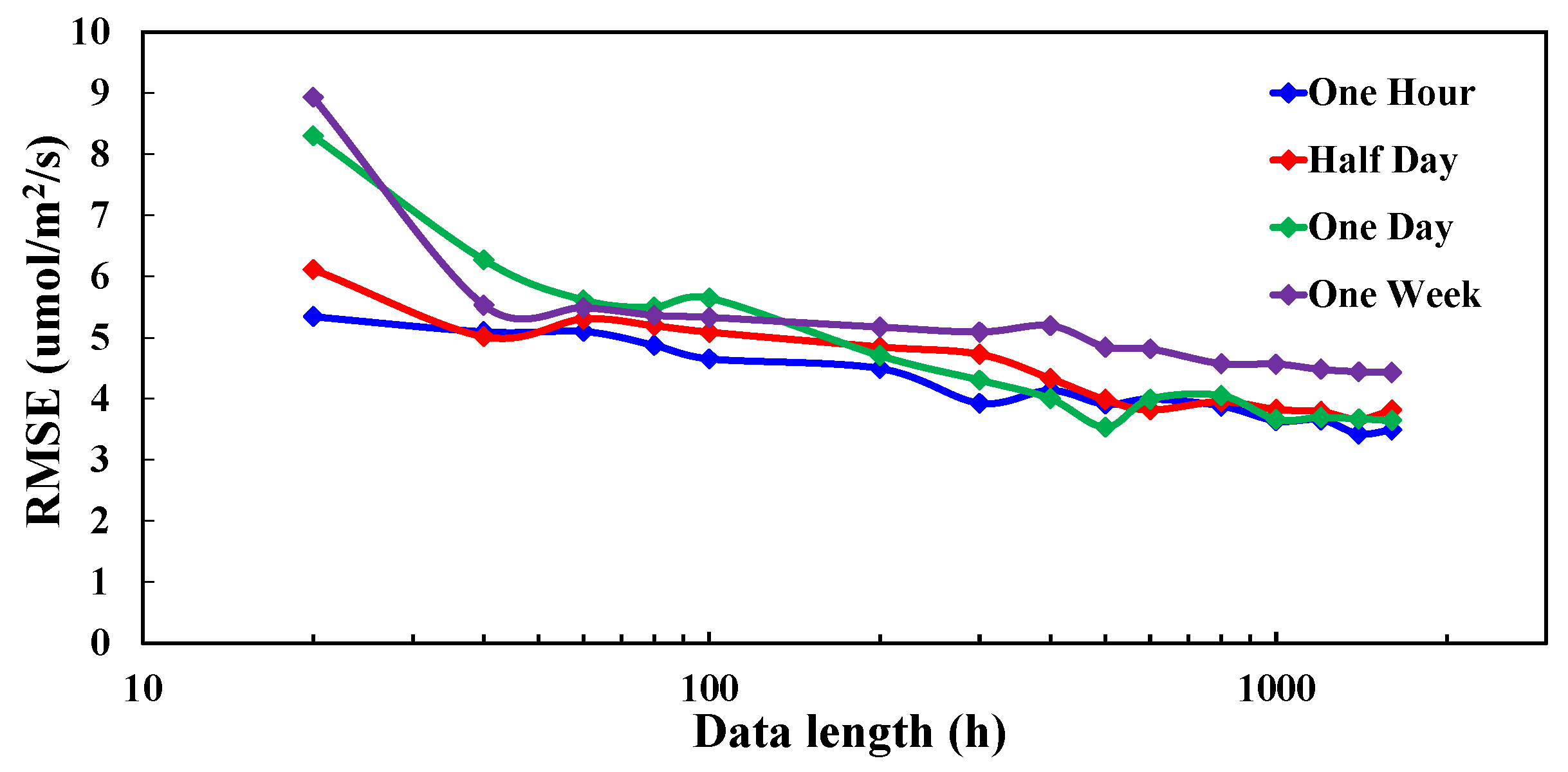
4.4. Effect of Data Length on Flux Gap-Filling
- (1)
- The gap-filling accuracy increased with the increase of data length and reached the model limitation when the data length is longer than 1300 h, except for the one hour gap length case.
- (2)
- For cases of one hour, the best model performance happened at different data lengths for different ecosystems (around 300, 900, and 500 h for grassland, rice paddy, and forest, respectively).
- (1)
- For all three sites, the RMSE curve of half day and one day gap lengths had the highest value at the beginning and then dropped as the data length increased; after a local RMSE minimum was reached, the RMSE oscillated up and down with the increase of data length and then reached its minimum at around 1300 h and remained stable till the end at 1600 h. The one week gap length case at the grassland also followed this trend.
- (2)
- For the one week gap length case at both the rice paddy field and forest, the RMSE decreased with the increase of data length and had the minimum after 1300 h.
- (3)
- For the one hour gap length case, the RMSE curve trend differed from each ecosystem. The minimum RMSE occurred at around 1000, 200, and 300 h for the grassland, rice paddy field, and forest, respectively.
- (4)
- Figure 9c shows that too much training data could result in a decrease in gap-filling accuracy for the short gap length cases (one hour, half day, and one day). This is because too much training data might average out the necessary features (e.g., peak values) of a short period.
5. Conclusions
- (1)
- In addition to the mean meteorological parameters, including the time factors (i.e., Julian day and decimal time) is important for all fluxes of CO2, water vapor, and sensible heat at the rice paddy field. However, the influences of time factors on these three fluxes are small (less than 5%) at the grassland. For the forest, this influence on CO2 flux is small, but it is larger for water vapor and sensible heat fluxes.
- (2)
- The hysteresis factors have no influence on all three fluxes at the grassland site. For the rice paddy, this influence on CO2 flux is not important, but it is important for water vapor and sensible heat fluxes. For the forest site, the hysteresis influence is important on CO2 flux, but it is small on both water vapor and sensible heat fluxes.
- (3)
- For all three ecosystems, the five ML models produced similar results for gap-filling of CO2, water vapor, and sensible heat fluxes. A list of the best ML model for flux gap-filling at the three sites is provided in Table 9. All in all, the SVM model is the most recommended model.
- (4)
- In terms of water vapor flux gap-filling, the ML model was better than the P–M equation, especially for forests; however, historical data are required a priori for training ML models.
- (5)
- The following general rule for the relation between gap length and data length of training can be made: if the gap length is less than one week, the training data length for achieving the best model performance is around 1300 h (i.e., 7.7 times the gap length).
- (6)
- For a particular gap that we are concerned about (especially where the flux peak values occurred), if training data length longer than 1300 h are not available when doing gap-filling, the data length listed in Table 11 is recommended.
Author Contributions
Funding
Acknowledgments
Conflicts of Interest
Appendix A. Brief Introduction of the Grid-Search Method
Appendix B. Calculation of the Stomatal Resistance (rst)
Appendix C. Summary of Individual Model Performance with and without Time Factors and Hysteresis Factors

| Flux | Model | RMSE | MAE | R2 | CE |
|---|---|---|---|---|---|
| CO2 | SVM | 4.90 (5.04) (4.90) | 3.02 (3.16) (3.02) | 0.60 (0.58) (0.60) | 0.60 (0.58) (0.60) |
| RF | 4.86 (5.06) (4.86) | 3.03 (3.22) (3.03) | 0.61 (0.57) (0.61) | 0.61 (0.57) (0.61) | |
| MLP | 4.96 (5.14) (4.96) | 3.19 (3.31) (3.19) | 0.59 (0.56) (0.59) | 0.59 (0.56) (0.59) | |
| DNN | 5.06 (5.16) (5.06) | 3.16 (3.31) (3.16) | 0.57 (0.56) (0.57) | 0.57 (0.55) (0.57) | |
| LSTM | 4.93 (5.10) (4.93) | 3.06 (3.23) (3.06) | 0.60 (0.57) (0.60) | 0.59 (0.56) (0.59) | |
| LE | SVM | 23.01 (23.01) (23.01) | 13.23 (13.23) (13.23) | 0.85 (0.85) (0.85) | 0.85 (0.85) (0.85) |
| RF | 24.88 (25.07) (24.88) | 14.72 (14.88) (14.72) | 0.83 (0.83) (0.83) | 0.83 (0.83) (0.83) | |
| MLP | 23.13 (23.13) (23.13) | 13.24 (13.24) (13.24) | 0.85 (0.85) (0.85) | 0.85 (0.85) (0.85) | |
| DNN | 22.92 (23.23) (22.92) | 13.19 (13.57) (13.19) | 0.86 (0.85) (0.86) | 0.85 (0.85) (0.85) | |
| LSTM | 22.76 (22.76) (22.76) | 12.99 (12.99) (12.99) | 0.86 (0.86) (0.86) | 0.86 (0.86) (0.86) | |
| H | SVM | 16.16 (16.28) (16.16) | 10.33 (10.38) (10.33) | 0.84 (0.84) (0.84) | 0.84 (0.84) (0.84) |
| RF | 16.66 (17.16) (16.66) | 10.54 (10.89) (10.54) | 0.83 (0.82) (0.83) | 0.83 (0.82) (0.83) | |
| MLP | 17.33 (17.35) (17.33) | 11.37 (11.28) (11.37) | 0.82 (0.82) (0.82) | 0.82 (0.82) (0.82) | |
| DNN | 16.87 (17.37) (16.87) | 10.79 (11.35) (10.79) | 0.83 (0.82) (0.83) | 0.83 (0.82) (0.83) | |
| LSTM | 16.63 (16.85) (16.63) | 10.80 (10.90) (10.80) | 0.83 (0.83) (0.83) | 0.83 (0.83) (0.83) |
| Flux | Model | RMSE | MAE | R2 | CE |
|---|---|---|---|---|---|
| CO2 | SVM | 2.27 (2.63) (2.27) | 1.70 (1.97) (1.70) | 0.90 (0.87) (0.90) | 0.89 (0.85) (0.89) |
| RF | 2.55 (2.66) (2.66) | 1.86 (1.99) (1.98) | 0.89 (0.87) (0.87) | 0.86 (0.84) (0.84) | |
| MLP | 2.30 (2.83) (2.30) | 1.71 (2.16) (1.74) | 0.90 (0.86) (0.90) | 0.88 (0.82) (0.88) | |
| DNN | 2.56 (3.99) (2.59) | 1.95 (3.08) (1.99) | 0.89 (0.87) (0.89) | 0.86 (0.64) (0.85) | |
| LSTM | 2.40 (2.94) (2.50) | 1.80 (2.32) (1.87) | 0.89 (0.86) (0.90) | 0.87 (0.81) (0.86) | |
| LE | SVM | 17.41 (18.64) (20.69) | 11.92 (12.26) (14.30) | 0.90 (0.89) (0.86) | 0.90 (0.89) (0.86) |
| RF | 19.85 (21.14) (20.79) | 13.32 (13.90) (14.21) | 0.87 (0.86) (0.86) | 0.87 (0.86) (0.86) | |
| MLP | 18.29 (20.88) (19.95) | 12.74 (14.23) (14.10) | 0.89 (0.86) (0.87) | 0.89 (0.86) (0.87) | |
| DNN | 18.79 (20.88) (20.30) | 13.28 (14.23) (14.37) | 0.89 (0.86) (0.87) | 0.88 (0.86) (0.87) | |
| LSTM | 18.20 (19.70) (20.52) | 12.79 (12.99) (14.50) | 0.89 (0.87) (0.86) | 0.89 (0.87) (0.86) | |
| H | SVM | 9.71 (10.92) (11.47) | 6.07 (6.74) (6.80) | 0.89 (0.86) (0.85) | 0.89 (0.86) (0.85) |
| RF | 9.64 (11.79) (9.70) | 6.06 (7.19) (6.08) | 0.89 (0.84) (0.89) | 0.89 (0.84) (0.89) | |
| MLP | 10.64 (11.93) (11.48) | 6.75 (7.58) (7.21) | 0.87 (0.84) (0.85) | 0.87 (0.83) (0.85) | |
| DNN | 12.05 (13.92) (13.58) | 7.35 (8.84) (8.40) | 0.83 (0.78) (0.79) | 0.83 (0.77) (0.79) | |
| LSTM | 10.00 (11.32) (10.78) | 6.43 (7.01) (6.74) | 0.89 (0.85) (0.87) | 0.88 (0.85) (0.86) |
| Flux | Model | RMSE | MAE | R2 | CE |
|---|---|---|---|---|---|
| CO2 | SVM | 3.40 (3.52) (3.68) | 2.30 (2.37) (2.52) | 0.81 (0.80) (0.78) | 0.81 (0.80) (0.78) |
| RF | 3.37 (3.45) (3.71) | 2.25 (2.33) (2.48) | 0.81 (0.81) (0.78) | 0.81 (0.81) (0.78) | |
| MLP | 3.46 (3.61) (3.80) | 2.40 (2.52) (2.66) | 0.80 (0.79) (0.77) | 0.80 (0.79) (0.76) | |
| DNN | 3.52 (3.59) (3.79) | 2.38 (2.50) (2.61) | 0.80 (0.79) (0.77) | 0.80 (0.79) (0.76) | |
| LSTM | 3.38 (3.48) (3.66) | 2.25 (2.38) (2.54) | 0.81 (0.80) (0.78) | 0.81 (0.80) (0.78) | |
| LE | SVM | 50.90 (55.73) (52.76) | 35.09 (38.50) (36.07) | 0.73 (0.68) (0.72) | 0.73 (0.67) (0.71) |
| RF | 53.05 (58.21) (53.21) | 36.42 (41.47) (36.62) | 0.70 (0.64) (0.70) | 0.70 (0.64) (0.70) | |
| MLP | 52.55 (57.32) (52.75) | 37.47 (40.44) (37.79) | 0.71 (0.66) (0.71) | 0.71 (0.65) (0.71) | |
| DNN | 54.06 (57.87) (54.26) | 37.89 (41.21) (38.94) | 0.69 (0.65) (0.69 | 0.69 (0.65) (0.69 | |
| LSTM | 52.04 (55.92) (54.16) | 36.67 (38.95) (36.97) | 0.72 (0.68) (0.69) | 0.72 (0.67) (0.69) | |
| H | SVM | 60.42 (65.57) (60.74) | 39.83 (42.54) (39.36) | 0.85 (0.82) (0.85) | 0.85 (0.82) (0.85) |
| RF | 60.96 (65.59) (61.48) | 40.61 (43.61) (40.71) | 0.85 (0.82) (0.85) | 0.85 (0.82) (0.85) | |
| MLP | 61.03 (64.28) (61.47) | 41.34 (43.67) (41.82) | 0.85 (0.83) (0.84) | 0.85 (0.83) (0.84) | |
| DNN | 64.76 (68.97) (67.82) | 44.82 (46.18) (44.32) | 0.83 (0.80) (0.81) | 0.83 (0.80) (0.81) | |
| LSTM | 61.67 (68.28) (62.72) | 39.95 (44.45) (41.01) | 0.84 (0.81) (0.84) | 0.84 (0.81) (0.84) |
Appendix D. Model Performance with and without Leaf Area Index (LAI)
| Flux | Model | RMSE | MAE | R2 | CE |
|---|---|---|---|---|---|
| CO2 Flux | SVM | 2.27 | 1.70 | 0.90 | 0.89 |
| (umol/m2/s) | SVM with LAI | 2.54 | 1.87 | 0.90 | 0.86 |
| Latent Heat Flux | SVM | 17.41 | 11.92 | 0.90 | 0.90 |
| (W/m2) | SVM with LAI | 16.29 | 10.78 | 0.91 | 0.91 |
| Sensible Heat Flux | SVM | 9.71 | 6.07 | 0.89 | 0.89 |
| (W/m2) | SVM with LAI | 9.75 | 6.10 | 0.89 | 0.89 |
Appendix E. Gap Scenario with Equal Total Gap Length

References
- Falge, E.; Baldocchi, D.; Olson, R.J.; Anthoni, P.; Aubinet, M.; Bernhofer, C.; Burba, G.; Ceulemans, R.; Clement, R.; Dolman, H.; et al. Gap filling strategies for defensible annual sums of net ecosystem exchange. Agric. For. Meteorol. 2001, 107, 43–69. [Google Scholar] [CrossRef] [Green Version]
- Moffat, A.M.; Papale, D.; Reichstein, M.; Hollinger, D.Y.; Richardson, A.D.; Barr, A.G.; Beckstein, C.; Braswell, B.H.; Churkina, G.; Desai, A.R.; et al. Comprehensive comparison of gap-filling techniques for eddy covariance net carbon fluxes. Agric. For. Meteorol. 2007, 147, 209–232. [Google Scholar] [CrossRef]
- Barr, A.G.; Black, T.A.; Hogg, E.H.; Kljun, N.; Morgenstern, K.; Nesic, Z. Inter-annual variability in the leaf area index of a boreal aspen-hazelnut forest in relation to net ecosystem production. Agric. For. Meteorol. 2004, 126, 237–255. [Google Scholar] [CrossRef]
- Desai, A.R.; Bolstad, P.; Cook, B.D.; Davis, K.J.; Carey, E.V. Comparing net ecosystem exchange of carbon dioxide between an old-growth and mature forest in the upper Midwest, USA. Agric. For. Meteorol. 2005, 128, 33–55. [Google Scholar] [CrossRef]
- Hollinger, D.Y.; Aber, J.; Dail, B.; Davidson, E.A.; Goltz, S.M.; Hughes, H.; Leclerc, M.; Lee, J.T.; Richardson, A.D.; Rodrigues, C.; et al. Spatial and temporal variability in forest-atmosphere CO2 exchange. Glob. Chang. Biol. 2004, 10, 1689–1706. [Google Scholar] [CrossRef]
- Noormets, A.; Chen, J.; Crow, T.R. Age-dependent changes in ecosystem carbon fluxes in managed forests in northern Wisconsin, USA. Ecosystems 2007, 10, 187–203. [Google Scholar] [CrossRef]
- Richardson, A.D.; Braswell, B.H.; Hollinger, D.Y.; Burman, P.; Davidson, E.A.; Evans, R.S.; Flanagan, L.B.; Munger, J.W.; Savage, K.; Urbanski, S.P.; et al. Comparing simple respiration models for eddy flux and dynamic chamber data. Agric. For. Meteorol. 2006, 141, 219–234. [Google Scholar] [CrossRef]
- Richardson, A.D.; Hollinger, D.Y. Statistical modeling of ecosystem respiration using eddy covariance data: Maximum likelihood parameter estimation, and Monte Carlo simulation of model and parameter uncertainty, applied to three simple models. Agric. For. Meteorol. 2005, 131, 191–208. [Google Scholar] [CrossRef]
- Stauch, V.J.; Jarvis, A.J. A semi-parametric model for eddy covariance CO2 flux time series data. Glob. Chang. Biol. 2006, 12, 1707–1716. [Google Scholar] [CrossRef]
- Hui, D.; Wan, S.; Su, B.; Katul, G.; Monson, R.; Luo, Y. Gap-filling missing data in eddy covariance measurements using multiple imputation (MI) for annual estimations. Agric. For. Meteorol. 2004, 121, 93–111. [Google Scholar] [CrossRef]
- Du, Q.; Liu, H.; Feng, J.; Wang, L. Effects of different gap filling methods and land surface energy balance closure on annual net ecosystem exchange in a semiarid area of China. Sci. China Earth Sci. 2014, 57, 1340–1351. [Google Scholar] [CrossRef]
- Van Wijk, M.T.; Bouten, W. Water and carbon fluxes above European coniferous forests modelled with artificial neural networks. Ecol. Model. 1999, 120, 181–197. [Google Scholar] [CrossRef]
- Carrara, A.; Kowalski, A.S.; Neirynck, J.; Janssens, I.A.; Yuste, J.C.; Ceulemans, R. Net ecosystem CO2 exchange of mixed forest in Belgium over 5 years. Agric. For. Meteorol. 2003, 119, 209–227. [Google Scholar] [CrossRef]
- Schmidt, A.; Wrzesinsky, T.; Klemm, O. Gap Filling and Quality Assessment of CO2 and Water Vapour Fluxes above an Urban Area with Radial Basis Function Neural Networks. Bound.-Layer Meteorol. 2008, 126, 389–413. [Google Scholar] [CrossRef]
- Kordowski, K.; Kuttler, W. Carbon dioxide fluxes over an urban park area. Atmos. Environ. 2010, 44, 2722–2730. [Google Scholar] [CrossRef]
- Papale, D.; Valentini, R. A new assessment of European forests carbon exchanges by eddy fluxes and artificial neural network spatialization. Glob. Chang. Biol. 2003, 9, 525–535. [Google Scholar] [CrossRef]
- Van Wijk, M.T.; Bouten, W.; Verstraten, J.M. Comparison of different modelling strategies for simulating gas exchange of a Douglas-fir forest. Ecol. Model. 2002, 158, 63–81. [Google Scholar] [CrossRef]
- Dengel, S.; Zona, D.; Sachs, T.; Aurela, M.; Jammet, M.; Parmentier, F.J.W.; Oechel, W.; Vesala, T. Testing the applicability of neural networks as a gap-filling method using CH4 flux data from high latitude wetlands. Biogeosciences 2013, 10, 8185–8200. [Google Scholar] [CrossRef] [Green Version]
- Nguyen, P.; Halem, M. Deep Learning Models for Predicting CO2 Flux Employing Multivariate Time Series; Mile TS: Anchorage, AK, USA, 2019. [Google Scholar]
- Kim, Y.; Johnson, M.S.; Knox, S.H.; Black, T.A.; Dalmagro, H.J.; Kang, M.; Kim, J.; Baldocchi, D. Gap-filling approaches for eddy covariance methane fluxes: A comparison of three machine learning algorithms and a traditional method with principal component analysis. Glob. Chang. Biol. 2020, 26, 1499–1518. [Google Scholar] [CrossRef]
- Kang, M.; Ichii, K.; Kim, J.; Indrawati, Y.M.; Park, J.; Moon, M.; Lim, J.H.; Chun, J.H. New Gap-Filling Strategies for Long-Period Flux Data Gaps Using a Data-Driven Approach. Atmosphere 2019, 10, 568. [Google Scholar] [CrossRef] [Green Version]
- Jaksic, V.; Kiely, G.; Albertson, J.; Oren, R.; Katul, G.; Leahy, P.; Byrne, K.A. Net ecosystem exchange of grassland in contrasting wet and dry years. Agric. For. Meteorol. 2006, 139, 323–334. [Google Scholar] [CrossRef]
- Hsieh, C.I.; Kiely, G.; Birkby, A.; Katul, G. Photosynthetic responses of a humid grassland ecosystem to future climate perturbations. Adv. Water Resour. 2005, 28, 910–916. [Google Scholar] [CrossRef]
- Aubinet, M.; Grelle, A.; Ibrom, A.; Rannik, Ü.; Moncrieff, J.; Foken, T.; Kowalski, A.S.; Marin, P.H.; Berbigier, P.; Bernhofer, C.; et al. Estimates of the annual net carbon and water exchange of forests: The EUROFLUX methodology. Adv. Ecol. Res. 2000, 30, 113–175. [Google Scholar] [CrossRef]
- Chu, H.S.; Chang, S.C.; Klemm, O.; Lai, C.W.; Lin, Y.Z.; Wu, C.C.; Lin, J.Y.; Jiang, J.Y.; Chen, J.; Gottgens, J.F.; et al. Does canopy wetness matter? Evapotranspiration from a subtropical montane cloud forest in Taiwan. Hydrol. Process. 2012, 28. [Google Scholar] [CrossRef]
- Lerman, P.M. Fitting segmented regression models by grid search. J. R. Stat. Soc. Ser. C (Appl. Stat.) 1980, 29, 77–84. [Google Scholar] [CrossRef]
- Cortes, C.; Vapnik, V. Support-vector networks. Mach. Learn. 1995, 20, 273–297. [Google Scholar] [CrossRef]
- Breiman, L. Random forests. Mach. Learn. 2001, 45, 5–32. [Google Scholar] [CrossRef] [Green Version]
- Rumelhart, D.E.; Hinton, G.E.; Williams, R.J. Learning representations by back-propagating errors. Nature 1986, 323, 533–536. [Google Scholar] [CrossRef]
- Kingma, D.P.; Ba, J. Adam: A method for stochastic optimization. arXiv 2014, arXiv:1412.6980. [Google Scholar]
- Baldi, P.; Sadowski, P.J. Understanding dropout. In Advances in Neural Information Processing Systems; MIT Press: Cambridge, MA, USA, 2013; pp. 2814–2822. [Google Scholar]
- Hinton, G.E.; Osindero, S.; Teh, Y.W. A fast learning algorithm for deep belief nets. Neural Comput. 2006, 18, 1527–1554. [Google Scholar] [CrossRef]
- Hochreiter, S.; Schmidhuber, J. Long short-term memory. Neural Comput. 1997, 9, 1735–1780. [Google Scholar] [CrossRef] [PubMed]
- Parascandolo, G.; Huttunen, H.; Virtanen, T. Recurrent neural networks for polyphonic sound event detection in real life recordings. In Proceedings of the 2016 IEEE International Conference on Acoustics, Speech and Signal Processing (ICASSP), Shanghai, China, 20–25 March 2016; pp. 6440–6444. [Google Scholar] [CrossRef] [Green Version]
- Yang, Y.; Dong, J.; Sun, X.; Lima, E.; Mu, Q.; Wang, X. A CFCC-LSTM model for sea surface temperature prediction. IEEE Geosci. Remote Sens. Lett. 2017, 15, 207–211. [Google Scholar] [CrossRef]
- Irmak, S.; Mutiibwa, D. On the dynamics of canopy resistance: Generalized linear estimation and relationships with primary micrometeorological variables. Water Resour. Res. 2010, 46. [Google Scholar] [CrossRef] [Green Version]
- Cui, Y.; Liu, Y.; Gan, G.; Wang, R. Hysteresis behavior of surface water fluxes in a hydrologic transition of an ephemeral Lake. J. Geophys. Res. Atmos. 2020, 125, e2019JD032364. [Google Scholar] [CrossRef]
- Lin, B.S.; Lei, H.; Hu, M.C.; Visessri, S.; Hsieh, C.I. Canopy Resistance and Estimation of Evapotranspiration above a Humid Cypress Forest. Adv. Meteorol. 2020, 2020, 4232138. [Google Scholar] [CrossRef]
- Zhang, Q.; Manzoni, S.; Katul, G.; Porporato, A.; Yang, D. The hysteretic evapotranspiration—vapor pressure deficit relation. J. Geophys. Res. Biogeosciences 2014, 119, 125–140. [Google Scholar] [CrossRef]


| Input Factors | Abbreviation | Definition |
|---|---|---|
| Time factors | JD | Julian day |
| DN | Day and night time index, which converts 24 h in a day to a continuous value from 0 to 1. | |
| Meteorological | Ta(t) | air temperature at time t (°C) |
| factors | RH(t) | relative humidity at time t (%) |
| Rn(t) | net radiation at time t (W/m2) | |
| U(t) | wind speed at time t (m/s) | |
| Hysteresis | Rn(t − 1) | net radiation at time t − 1 (i.e., 30 min before time t) (W/m2) |
| factors | Rn(t − 2) | net radiation at time t − 2 (i.e., one hour before time t) (W/m2) |
| Ta(t − 1) | air temperature at time t − 1 (°C) | |
| Ta(t − 2) | air temperature at time t − 2 (°C) | |
| Tavg(t) | average of the air temperatures measured at time t, t − 1, and t − 2 (°C) |
| Model | Study Site | Optimal Input Combinations |
|---|---|---|
| SVM | Grassland | JD, DN, Ta(t),RH, Rn(t), U(t) |
| Rice paddy field | JD, DN, Ta(t), Rn(t), U(t) | |
| Forest | JD, DN, Ta(t), RH, Rn(t), Rn(t−2), Rn(t−1), Ta(t−2), Ta(t−1) | |
| RF | Grassland | JD, DN, Ta(t), RH, Rn(t), U(t) |
| Rice paddy field | DN, Ta(t), RH, Rn(t), U(t), Rn(t−2), Rn(t−1), Ta(t−2), Ta(t−1), Tavg(t) | |
| Forest | JD, DN, Ta(t), RH, Rn(t), U(t), Rn(t−2), Rn(t−1), Ta(t−2), Ta(t−1), Tavg(t) | |
| MLP | Grassland | JD, DN, Ta(t), RH, Rn(t), U(t) |
| Rice paddy field | JD, DN, Ta(t), Rn(t), U(t), Rn (t−1), Tavg(t) | |
| Forest | JD, DN, Ta(t), RH, Rn(t), U(t), Rn(t−2), Rn(t−1), Ta(t−1), Tavg(t) | |
| DNN | Grassland | JD, Ta(t), RH, Rn(t), U(t) |
| Rice paddy field | JD, DN, Ta(t), RH, Rn(t), U(t), Rn(t−2), Rn(t−1), Ta(t−2), Ta(t−1), Tavg(t) | |
| Forest | JD, DN, Ta(t), RH, Rn(t), U(t), Rn(t−2), Rn(t−1), Ta(t−2), Ta(t−1), Tavg(t) | |
| LSTM | Grassland | JD, DN, Ta(t), RH, Rn(t), U(t) |
| Rice paddy field | JD, DN, Ta(t), Rn(t), U(t), Rn(t−2), Rn(t−1), Ta(t−2), Ta(t−1), Tavg(t) | |
| Forest | JD, DN, Ta(t), RH, Rn(t), U(t), Rn(t−2), Rn(t−1), Ta(t−2), Ta(t−1), |
| Model | Study Site | Optimal Input Combinations |
|---|---|---|
| SVM | Grassland | Ta(t), RH, Rn(t), U(t) |
| Rice paddy field | JD, DN, Ta(t), RH, Rn(t), U(t), Rn(t−2), Rn(t−1), Ta(t−2), Ta(t−1), Tavg(t) | |
| Forest | JD, DN, Ta(t), RH, Rn(t), Rn(t−2), Rn(t−1), Ta(t−2), Ta(t−1), Tavg(t) | |
| RF | Grassland | DN, Ta(t), Rn(t), U(t) |
| Rice paddy field | JD, DN, Ta(t), RH, Rn(t), U(t), Rn(t−2), Rn(t−1), Ta(t−2), Ta(t−1), Tavg(t) | |
| Forest | JD, DN, Ta(t), RH, Rn(t), U(t), Rn(t−1), Tavg(t) | |
| MLP | Grassland | Ta(t), RH, Rn(t), U(t) |
| Rice paddy field | JD, Ta(t), Rn(t), U(t), Rn(t−2), Rn(t−1), Ta(t−2), Ta(t−1), Tavg(t) | |
| Forest | JD, DN, Ta(t), RH, Rn(t), U(t), Rn(t−1), Tavg(t) | |
| DNN | Grassland | DN, Ta(t), RH, Rn(t), U(t) |
| Rice paddy field | JD, DN, Ta(t), RH, Rn(t), U(t), Rn(t−2), Rn(t−1), Ta(t−2), Ta(t−1), Tavg(t) | |
| Forest | JD, DN, Ta(t), RH, Rn(t), U(t), Rn(t−2), Rn(t−1), Ta(t−2), Ta(t−1), Tavg(t) | |
| LSTM | Grassland | Ta(t), RH, Rn(t), U(t) |
| Rice paddy field | JD, DN, Ta(t), RH, Rn(t), U(t), Rn(t−2), Rn(t−1), Ta(t−2), Ta(t−1), Tavg(t) | |
| Forest | JD, DN, Ta(t), RH, Rn(t), U(t), Rn(t−2), Rn(t−1), Ta(t−2), Ta(t−1), Tavg(t) |
| Model | Study Site | Optimal Input Combinations |
|---|---|---|
| SVM | Grassland | JD, DN, Ta(t), RH, Rn(t), U(t) |
| Rice paddy field | JD, DN, Ta(t), RH, Rn(t), U(t), Rn(t−2), Rn(t−1), Ta(t−2), Ta(t−1), Tavg(t) | |
| Forest | JD, DN, Ta(t), RH, Rn(t), U(t), Rn(t−1), Ta(t−1), Tavg(t) | |
| RF | Grassland | JD, Ta(t), RH, Rn(t), U(t) |
| Rice paddy field | JD, DN, Rn(t), U(t), Tavg(t) | |
| Forest | JD, DN, Ta(t), RH, Rn(t), U(t), Rn(t−1), Tavg(t) | |
| MLP | Grassland | JD, Ta(t), Rn(t), U(t) |
| Rice paddy field | JD, DN, Ta(t), RH, Rn(t), U(t), Rn(t−2), Rn(t−1), Ta(t−2), Ta(t−1), Tavg(t) | |
| Forest | JD, DN, Ta(t), RH, Rn(t), U(t), Rn(t−1), Ta(t−1), Tavg(t) | |
| DNN | Grassland | JD, Ta(t), Rn(t), U(t) |
| Rice paddy field | JD, DN, Ta(t), RH, Rn(t), U(t), Rn(t−2), Rn(t−1), Ta(t−2), Ta(t−1), Tavg(t) | |
| Forest | JD, DN, Ta(t), RH, Rn(t), U(t), Tavg(t) | |
| LSTM | Grassland | JD, Ta(t), RH, Rn(t), U(t) |
| Rice paddy field | JD, DN, Ta(t), RH, Rn(t), U(t), Rn(t−2), Rn(t−1), Ta(t−2), Ta(t−1), Tavg(t) | |
| Forest | JD, DN, Ta(t), RH, Rn(t), U(t), Tavg(t) |
| Flux | Type | RMSE | MAE | R2 | CE |
|---|---|---|---|---|---|
| CO2 flux | Model’s average | 4.94 | 3.09 | 0.59 | 0.59 |
| without time factors | 5.10 | 3.25 | 0.57 | 0.56 | |
| without hysteresis factors | 4.94 | 3.09 | 0.59 | 0.59 | |
| Improvement rate with time factors (%) | 3.10 | 4.74 | 4.58 | 4.96 | |
| Improvement rate with hysteresis factors (%) | 0.00 | 0.00 | 0.00 | 0.00 | |
| Latent heat flux | Model’s average | 23.34 | 13.47 | 0.85 | 0.85 |
| without time factors | 23.44 | 13.58 | 0.85 | 0.85 | |
| without hysteresis factors | 23.34 | 13.47 | 0.85 | 0.85 | |
| Improvement rate with time factors (%) | 0.43 | 0.80 | 0.24 | 0.00 | |
| Improvement rate with hysteresis factors (%) | 0.00 | 0.00 | 0.00 | 0.00 | |
| Sensible heat flux | Model’s average | 16.73 | 10.77 | 0.83 | 0.83 |
| without time factors | 17.00 | 10.96 | 0.83 | 0.83 | |
| without hysteresis factors | 16.73 | 10.77 | 0.83 | 0.83 | |
| Improvement rate with time factors (%) | 1.60 | 1.77 | 0.48 | 0.48 | |
| Improvement rate with hysteresis factors (%) | 0.00 | 0.00 | 0.00 | 0.00 |
| Flux | Type | RMSE | MAE | R2 | CE |
|---|---|---|---|---|---|
| CO2 flux | Model’s average | 2.42 | 1.80 | 0.89 | 0.87 |
| without time factors | 3.01 | 2.30 | 0.87 | 0.79 | |
| without hysteresis factors | 2.46 | 1.86 | 0.89 | 0.86 | |
| Improvement rate with time factors (%) | 19.73 | 21.70 | 3.23 | 10.10 | |
| Improvement rate with hysteresis factors (%) | 1.95 | 2.80 | 0.22 | 0.93 | |
| Latent heat flux | Model’s average | 18.51 | 12.81 | 0.89 | 0.89 |
| without time factors | 20.25 | 13.52 | 0.87 | 0.87 | |
| without hysteresis factors | 20.45 | 14.30 | 0.86 | 0.86 | |
| Improvement rate with time factors (%) | 8.59 | 5.27 | 2.30 | 2.31 | |
| Improvement rate with hysteresis factors (%) | 9.50 | 10.39 | 2.78 | 2.55 | |
| Sensible heat flux | Model’s average | 10.41 | 6.53 | 0.87 | 0.87 |
| without time factors | 11.98 | 7.47 | 0.83 | 0.83 | |
| without hysteresis factors | 11.40 | 7.05 | 0.85 | 0.85 | |
| Improvement rate with time factors (%) | 13.09 | 12.58 | 4.80 | 5.06 | |
| Improvement rate with hysteresis factors (%) | 8.72 | 7.29 | 2.82 | 2.83 |
| Flux | Type | RMSE | MAE | R2 | CE |
|---|---|---|---|---|---|
| CO2 flux | Model’s average | 3.43 | 2.32 | 0.81 | 0.81 |
| without time factors | 3.53 | 2.42 | 0.80 | 0.80 | |
| without hysteresis factors | 3.73 | 2.56 | 0.78 | 0.77 | |
| Improvement rate with time factors (%) | 2.95 | 4.30 | 1.00 | 1.00 | |
| Improvement rate with hysteresis factors (%) | 8.10 | 9.60 | 3.87 | 4.40 | |
| Latent heat flux | Model’s average | 52.52 | 36.71 | 0.71 | 0.71 |
| without time factors | 57.01 | 40.11 | 0.66 | 0.66 | |
| without hysteresis factors | 53.43 | 37.28 | 0.70 | 0.70 | |
| Improvement rate with time factors (%) | 7.88 | 8.49 | 7.25 | 8.23 | |
| Improvement rate with hysteresis factors (%) | 1.70 | 1.53 | 1.14 | 1.43 | |
| Sensible heat flux | Model’s average | 61.77 | 41.31 | 0.84 | 0.84 |
| without time factors | 66.54 | 44.09 | 0.82 | 0.82 | |
| without hysteresis factors | 62.85 | 41.44 | 0.84 | 0.84 | |
| Improvement rate with time factors (%) | 7.17 | 6.31 | 3.43 | 3.43 | |
| Improvement rate with hysteresis factors (%) | 1.72 | 0.32 | 0.96 | 0.96 |
| CO2 Flux | Latent Heat Flux | Sensible Heat Flux | ||||||||
|---|---|---|---|---|---|---|---|---|---|---|
| Site | Model | a | b | R2 | a | b | R2 | a | b | R2 |
| Grassland | SVM | 1.14 | 0.14 | 0.60 | 0.99 | −0.26 | 0.85 | 1.02 | 0.16 | 0.84 |
| RF | 1.10 | −0.10 | 0.61 | 1.02 | −1.15 | 0.83 | 1.03 | −0.10 | 0.83 | |
| MLP | 1.00 | 0.05 | 0.59 | 1.01 | −0.33 | 0.85 | 1.01 | 0.12 | 0.82 | |
| DNN | 1.02 | −0.03 | 0.57 | 0.98 | −0.63 | 0.86 | 1.03 | 5.34 | 0.83 | |
| LSTM | 1.07 | 0.41 | 0.60 | 1.02 | −1.86 | 0.86 | 1.05 | 1.33 | 0.83 | |
| Rice paddy | SVM | 1.06 | −0.16 | 0.91 | 0.98 | 1.33 | 0.90 | 1.00 | 0.10 | 0.89 |
| field | RF | 1.06 | 0.21 | 0.89 | 0.93 | 3.41 | 0.87 | 1.03 | −0.32 | 0.89 |
| MLP | 1.03 | −0.02 | 0.90 | 0.91 | 4.43 | 0.89 | 1.00 | 0.02 | 0.87 | |
| DNN | 0.99 | 0.57 | 0.89 | 0.97 | 3.23 | 0.89 | 1.04 | 0.08 | 0.83 | |
| LSTM | 0.94 | 0.08 | 0.89 | 0.92 | 4.11 | 0.89 | 0.99 | 0.61 | 0.89 | |
| Forest | SVM | 1.00 | 0.07 | 0.81 | 1.03 | 1.34 | 0.76 | 1.01 | 0.49 | 0.85 |
| RF | 1.02 | −1.27 | 0.81 | 1.08 | −8.68 | 0.70 | 1.02 | −3.74 | 0.85 | |
| MLP | 0.98 | −0.02 | 0.80 | 1.00 | −0.99 | 0.71 | 0.99 | −0.03 | 0.85 | |
| DNN | 1.00 | 0.01 | 0.80 | 1.07 | 2.50 | 0.69 | 1.02 | −7.29 | 0.83 | |
| LSTM | 0.98 | −0.03 | 0.81 | 1.00 | 1.86 | 0.72 | 1.11 | −0.34 | 0.84 | |
| Site | CO2 Flux | Latent Heat Flux | Sensible Heat Flux |
|---|---|---|---|
| Grassland | RF | LSTM | SVM |
| Rice paddy field | SVM | SVM | SVM |
| Forest | SVM | SVM | SVM |
| Site | Model | RMSE (W/m2) | MAE (W/m2) | R2 | CE | a (Slope) | b (Intercept) |
|---|---|---|---|---|---|---|---|
| Grassland | LSTM | 22.76 | 12.99 | 0.86 | 0.86 | 1.02 | −1.23 |
| P−M equation | 28.19 | 20.33 | 0.82 | 0.78 | 1.12 | −17.02 | |
| Rice paddy | SVM | 17.41 | 11.92 | 0.90 | 0.90 | 0.98 | 1.33 |
| field | P−M equation | 13.32 | 9.50 | 0.95 | 0.94 | 1.07 | −8.51 |
| Forest | SVM | 50.90 | 35.09 | 0.76 | 0.73 | 1.03 | 1.34 |
| P−M equation | 67.73 | 46.27 | 0.59 | 0.54 | 0.86 | 28.95 |
| LE | CO2 | H | ||||||||||
|---|---|---|---|---|---|---|---|---|---|---|---|---|
| Site | One Hour | Half Day | One Day | One Week | One Hour | Half Day | One Day | One Week | One hour | Half Day | One Day | One Week |
| Grassland | 280 | 440 | 200 | 860 | 1120 | 100 | 80 | 240 | 640 | 620 | 620 | 1280 |
| Rice paddy field | 880 | 1380 | 1380 | 920 | 160 | 100 | 100 | 1340 | 1180 | 1180 | 1180 | 580 |
| Forest | 460 | 740 | 1120 | 460 | 280 | 200 | 1340 | 640 | 240 | 380 | 1080 | 1200 |
Publisher’s Note: MDPI stays neutral with regard to jurisdictional claims in published maps and institutional affiliations. |
© 2020 by the authors. Licensee MDPI, Basel, Switzerland. This article is an open access article distributed under the terms and conditions of the Creative Commons Attribution (CC BY) license (http://creativecommons.org/licenses/by/4.0/).
Share and Cite
Huang, I.-H.; Hsieh, C.-I. Gap-Filling of Surface Fluxes Using Machine Learning Algorithms in Various Ecosystems. Water 2020, 12, 3415. https://doi.org/10.3390/w12123415
Huang I-H, Hsieh C-I. Gap-Filling of Surface Fluxes Using Machine Learning Algorithms in Various Ecosystems. Water. 2020; 12(12):3415. https://doi.org/10.3390/w12123415
Chicago/Turabian StyleHuang, I-Hang, and Cheng-I Hsieh. 2020. "Gap-Filling of Surface Fluxes Using Machine Learning Algorithms in Various Ecosystems" Water 12, no. 12: 3415. https://doi.org/10.3390/w12123415