Abstract
Climate change, especially the trend towards global warming, will significantly affect the global hydrological cycle, leading to a general reduction of the water available for agriculture. In this scenario, it is essential that research should focus on the development of ‘water saving’ techniques and technologies. This work summarizes the methodology followed in a project for large scale implementation of variable rate irrigation (VRI) systems using center pivots in corn crop. This is based on technologies for monitoring (i) soil electrical conductivity (ECa) and altimetry, (ii) soil moisture content, (iii) vegetation indices (Normalized Difference Vegetation Index, NDVI) obtained from satellite images, and automatic pivot travel speed control technologies. ECa maps were the basis for the definition of first homogeneous management zones (HMZ) in an experimental corn field of 28 ha. NDVI time-series were used to establish the subsequent HMZ and the respective dynamic prescription irrigation maps. The main result of this study was the reduction of spatial yield variability with the VRI management in 2017 compared to the conventional irrigation management. This study demonstrates how a relatively simple approach could be designed and implemented on a large scale, which represents an important and sustainable contribution to the resolution of practical farmer issues.
1. Introduction
Today, agricultural activity develops in a context dominated by two challenges: productivity and sustainability. The increase in food production to satisfy all the demands of the 9 billion people (world population expected in the year 2050) is a challenge for agricultural professionals, who require the use of efficient techniques and technologies in all of their production processes [1]. In this context, the importance of irrigated agriculture is demonstrated by the fact that, while only 16% of the world’s cultivated area is irrigated, it is expected to produce 44% of world food by 2050 [1]. This scenario gains greater importance when climate variability, regulatory nutrient management, water conservation policies, and declining sources of compound challenges faces irrigated crop production [2]. Climate change will significantly affect the hydrological cycle leading, in many agricultural areas of the planet, to more frequent droughts and heat waves, to alteration of the spatial and temporal patterns of precipitation, to an increase in evapotranspiration, and to a general reduction in the availability of water for agriculture [3]. Given the increase cost of production factors (such as water) and increasing awareness of the need to preserve our natural environment, producers rely more on precision agriculture (PA) technologies to reduce economic costs and environmental impact [4]. PA methodology is a field management strategy that measures within the field variation of certain parameters, and then incorporates that variability into a differentiated application of resources to the file [5].
The importance of properly managing irrigation is a fundamental factor for sustainable production [6]. Similar to other agronomic inputs, the conventional management of water is based on the application of a homogeneous input over the field, considered as a uniform spatial unit. However, in any field, one can observe spatial heterogeneity of soil characteristics, topography, microclimate, crop development, water status, and yield, which result in spatial variability of irrigation efficiency and a non-uniform irrigation requirement [3,7].
With eight million hectares of the irrigated area, a center pivot system represents 23% of the total area irrigated by sprinkler irrigation systems [1]. Center pivot irrigation consists of the application of water through a moving lateral line with several water outlets supported on moving towers, which revolve around a fixed pivot point (center tower) and irrigate a circular area [1]. Variable rate irrigation (VRI), sometimes referred to as ‘precision’ or ‘site-specific’ irrigation, which is the capacity of an irrigation system to apply different amounts of water to different areas of the field based on site-specific needs, emerges as a potential solution to increase the productivity and reduce the environmental impact of irrigated agriculture [8,9]. The methods for VRI in centre pivots systems include: “speed or sector control” (variable speed irrigation, VSI), where the water application rate is varied in the direction of the moving sprinkler by varying its travel speed, and “zone control” (variable zone irrigation, VZI), which allows watering application rates to be varied along the lateral pipeline as well as in the direction of the sprinkler movement [2]. VSI does not require additional hardware on the pivot. It simply uses a more sophisticated control panel that will slow down or speed up the pivot to apply more or less water in different areas of the field and many of the newer pivot control panels already built into them since the overall pivot flow rate remains constant. A producer could transition to VSI first before deciding whether to invest in VZI, since the first, conceptually, may be easier to understand [2]. Despite variable speed irrigation’s clear limitations to variations only in pie-shaped wedges, VSI has a lower cost than VZI given that the only modifications to the pivot are to the electronic controls, resulting in a shorter period for return on investment [2].
VRI assumes that crop water needs to vary spatially. In fact, soil water content varies not only spatially but temporally [10]. In many fields, crop water needs are variable throughout an irrigation season [2] due to differences in soil water holding capacity [11], which requires dynamic irrigation prescription maps [10] to address the variability in the soil available water. Prescription maps, or plans, contain irrigation amounts that vary for the different areas of the field, and, in this case, they should also vary over time, i.e., irrigation decisions must be re-evaluated many times over a season, which corresponds to modify VRI prescriptions in a way that improves the overall profitability [2]. However, the data collection, analysis, and creation of optimal VRI prescriptions for a specific field’s needs can be complex, time consuming, and expensive, especially since many field situations require these prescriptions to vary both in time and in space [2]. A previous stage in this process involves the establishment of homogeneous management zones (HMZ) [2,4]. An HMZ is a sub-region of a field that is relatively homogeneous in terms of soil-landscape attributes [5]. It is critical to select appropriate attribute(s) and method to delineate robust zones, such as combining various types of data of several years, attending to temporal climatic variability, which have proved to be promising for the creation of HMZ [5]. Two different paradigms of monitoring field-level spatial variability have emerged and proved effective including one based on monitoring soil water properties and the other on monitoring the plant condition [7]. A field can be zoned based on a single soil-crop variable or multiple attributes, which are expected to affect yield. Advances in proximal and non-invasive sensing technology and data analysis techniques are now able to provide efficient information on soil, crops, and associated environmental properties [12]. Soil apparent electrical conductivity (ECa), yield maps, topography, and satellite images are among suggested attributes to delineate HMZ [2,9]. Application of remote sensing is especially attractive because it is non-invasive and relatively inexpensive [5]. Effective management of VRI will likely require a combination of both remote sensing and proximal sensing to detect spatially and temporally dynamic variable crop water needs [2]. In general, the following are recognized as necessary to sustain the adoption of site-specific VRI: (i) tools for defining HMZ, (ii) software to write basic prescriptions, (iii) decision support systems, and (iv) technical assistance and training [13].
The objective of this case study is to evaluate automatic center pivot travel speed control for dynamic management of irrigation in corn (Zea mays L.) based on technologies that monitor (i) soil electrical conductivity (ECa), (ii) yield maps, (iii) soil moisture, and (iv) vegetation indices (Normalized Difference Vegetation Index, NDVI) obtained from satellite images (Figure 1).
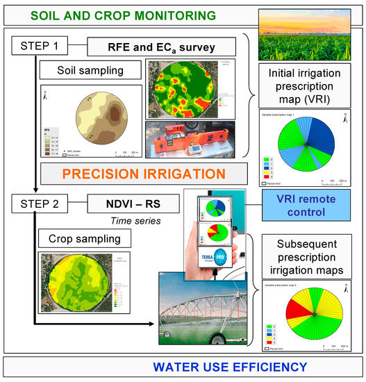
Figure 1.
Schematic representation of the methodology followed in this study.
2. Materials and Methods
2.1. Chronological Approach
Figure 1 schematically shows the approach followed in this study to evaluate automatic center pivot travel speed control for dynamic management of irrigation in corn. Figure 2 shows the chronological diagram of the tasks carried out between October 2016 and October 2017, which corresponds to the period between two consecutive crop harvests. In situ crop monitoring, year after year, allowed the farmer to identify areas with very different productivity, which served as the starting point of this study. Relative field elevation and soil ECa surveys, soil sampling, and NDVI monitoring were the basis for the definition of homogeneous management zones and, later, for the preparation of variable rate irrigation maps.
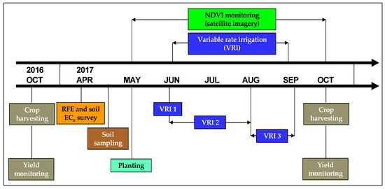
Figure 2.
Chronological diagram of the tasks carried in this study (NDVI—Normalized Difference Vegetation Index, VRI—Variable Rate Irrigation, RFE—Relative Field Elevation, ECa—Soil Electrical Conductivity Apparent).
2.2. Experimental Field
In this work, the corn field “Eucalyptus” of 28.2 ha, located at Samora Correia, near Lisbon, Portugal (38°50.68′ N; 8°52.55′ W), was monitored between October 2016 and October 2017. This farm is located in Lezíria do Ribatejo, a characteristic corn producing area under strong influence of the Tejo River Bay. The predominant soil in this parcel is classified as Fluvisols [14], sedimentary formations derived especially from recent fluvial deposits. These are soils with little or no profile differentiation but a distinct topsoil horizon, with good natural fertility, whereby many crops are grown, normally with some form of water control [14].
The Mediterranean climate is characterized by having most of the rainfall concentrated in the coldest months of December and January and very dry, hot summers, especially during the months of July and August, when corn is in full development. The average annual rainfall does not normally exceed 600 mm and the temperature in the summer can reach 40 °C. In this climatic context, the crop growth during the Spring-Summer period (May to October: planting to harvest) is sustained through regular irrigation.
2.3. Soil Apparent Electrical Conductivity and Altimetric Surveys
In April 2017, an ECa survey was carried out with an electromagnetic induction device (EM38; Geonic, Ltd., Mississauga, ON, Canada) (Figure 3a). This equipment consists of a receiver and a transmitter coil installed 1.0 m apart at the opposite ends of a nonconductive bar. The measured depth depends on the coil configuration (horizontal or vertical) and the distance between the coils. In this study, the ECa survey was measured at two depths: 0–0.50 m and 0–1.0 m. The sensor was transported by a platform (Figure 3b) and pulled by an all-terrain vehicle (Figure 3c) equipped with a global positioning system (GPS) receiver and data collection equipment, at a speed of approximately 12 km h−1. An offset of 10 m between successive parallel paths was guaranteed by a GPS driving support system. This GPS receiver also made it possible to collect the altimetric data for the preparation of the relative field elevation map.
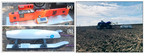
Figure 3.
Electromagnetic induction device (EM38) (a), transport platform, (b) and sensor in field work (c).
2.4. Soil Sampling
In this study, the ECa map was used to define the location of six soil sampling points, distributed by ECa gradients (areas with low ECa values, sampling points 1 and 4, intermediate ECa values, sampling points 2 and 3, and high ECa values, points 5 and 6) and different altimetry. The GPS georeferenced samples were collected using a gouge auger and a hammer, at a depth range of 0–0.30 m. Each composite sample resulted from eight sub-samples collected within a radius of 5 m in relation to the georeferenced point. The samples were then processed in the laboratory to determine the texture (sand, silt, and clay components), pH, organic matter, nitrogen, phosphorus, exchange bases (calcium, magnesium and sodium), iron, copper, manganese, and zinc. Standard methods of soil analytic determination [15] were used for all these parameters.
2.5. Vegetation Multispectral Measurements by Remote Sensing
Sentinel-2 optical images (freely available from the European Space Agency, ESA) were used. For this work, Sentinel-2 band 4 (B4, 10 m spatial resolution, 665 nm) and band 8 (B8, 10 m spatial resolution, 842 nm), atmospherically corrected imagery, were extracted from Copernicus data hub and used to calculate the normalized difference vegetation index (NDVI, Equation (1)) [16].
A preliminary processing was carried out on these records to remove outliers due to the presence of clouds. Only cloud-free images were used in the analysis. The monitoring of NDVI in the experimental field was carried out between May (date of planting) and October (date of harvest).
2.6. Definition of Homogeneous Management Zones (HMZ)
Homogeneous subfields were delineated using a fuzzy cluster algorithm [17]. The MZ Analyst (MZA) software (Microsoft Corp., Redmond, WA, United States) was utilized in this study. This software uses procedures for delineating MZs in a field and evaluating the number of homogeneous zones as described by Fridgen et al. [18]. Consequently, the fuzzy c-means, an unsupervised continuous classification procedure, which is implemented in the MZA program, was used to divide the field into different cluster classes. This classification algorithm is very adequate for grouping properties in the soil continuum because it produces a continuous grouping of objects by assigning partial class membership. Some clustering parameters need to be specified in the MZA program. The fuzziness exponent was set at the conventional value of 1.3 and the Mahalanobis measure of similarity was selected since it is the most suitable for multivariate data classification [19]. Three homogeneous zones were considered as, in all cases, the two indices used to evaluate the number of classes, the fuzziness performance index (FPI), and the normalized classification entropy (NCE) [18], which were between 0 and 1. FPI is a measure of the degree of membership sharing among classes: 0 indicates different classes with no membership sharing and 1 reflects a strong sharing of membership. NCE is an estimate of the amount of disorganization created by a number of classes: 0 indicates high organization and 1 represents a strong disorganization. When each index is at minimum, which indicates the least membership sharing (FPI) and greatest amount of organization (NCE) as a result of the clustering process, the optimum number of classes is achieved [18].
In this study, three MZ maps were defined, one initially based on soil ECa, altimetric surveys, and soil sampling, which has been redefined twice based on NDVI maps (14 June and 23 August) and implemented sequentially during the lifecycle of the crop, as described in the following section. The HMZ obtained from MZA software were later converted into the pie slice format, suitable for pivot irrigation. These new maps were generated by taking into account the area of each homogeneous zone that fall within each circular sector. The calculations were performed for each area corresponding to a slice with 6° amplitude in the irrigation perimeter, thus, totaling 60 slices.
2.7. Definition and Implementation of Variable Rate Irrigation (VRI) Maps
The HMZ defined in a pie slice format identified zones of greater and of lesser potential productivity, constituting the basis for farmer’s decision-making. In this work, the knowledge of a spatial variability pattern of 2016 corn yield influenced the farmer’s decision in terms of variable irrigation prescription. Corn yield maps of 2016 and 2017 were obtained by a service provider using a John Deere harvester equipped with a crop yield monitor (grain flow meter associated with a GPS receiver). As mentioned, in order to achieve the final goal of reducing the spatial variability of production in this field, three sequential VRI stages were implemented based on three distinct HMZ maps, with each optimized for a specific objective. The initial map was based on the soil ECa survey and soil sampling, and was optimized with the objective of stimulating the productivity of less fertile soils through a greater irrigation prescription. This map was then redefined based on NDVI measurements of 14 June with the objective of stimulating the productivity of the areas with lower vegetative vigour, and then redefined again based on the NDVI measurement of 23 August with the objective of saving water in areas where the crop had reached advanced stages of its vegetative cycle (Table 1). For the implementation of VRI maps in the 2017 campaign, an electronic “URAPIVOT Irrigation Systems” (Chamsa, Madrid, Spain) controller was used, running the “USENS” software application (app) developed by “TERRAPRO Technologies” (Samora Correia, Portugal), installed on a mobile device. The remote control of pivot travel speed was based on the VRI map, and the actual position (angle) of the pivot.

Table 1.
Steps, objectives, and expected results of homogeneous management zones (HMZ) and variable rate irrigation (VRI) maps.
The irrigation frequency was determined by the evolution of soil moisture content (SMC) monitored continuously by two SMC capacitance probes (“TERRAPRO Technologies,” Samora Correia, Portugal).
The reduction in the amounts of irrigation water (in %) resulting from the implementation of variable irrigation strategy in lieu of conventional and uniform prescription (“standard” or 100%), which can be calculated based on VRI maps, the number of irrigation events (n), and the established prescription classes (z). Equations (2) and (3) calculate the relative irrigation water amount (RIWA) as a weighted average of percentage of irrigation water used in each irrigation event (Ai), calculated as a weighted average of water amounts used in percentage of area (ai,j), where the weight of each value of “i” is given by the number of irrigation events (ni).
where: ni—Number of irrigation events. zj—Irrigation correction factor or amount of water as a percentage of standard prescription (prescription classes). ai,j—Relative area to each ni and zj data, as a percentage of the total irrigation area.
3. Results
Mean corn yield in 2016 was 10,510 ± 4689 kg ha−1 (CV = 44.6%). Figure 4 shows the spatial variability of corn yield at the “Eucalyptus” field with an evident contrast between high productivity areas (>13,000 kg ha−1) and low productivity areas (<5000 kg ha−1). This was the main motivating reason of this study with a purpose, on the one hand, to identify potential causes of low productivity and, on the other hand, to stimulate productivity in these areas, reducing the overall variability of the field.
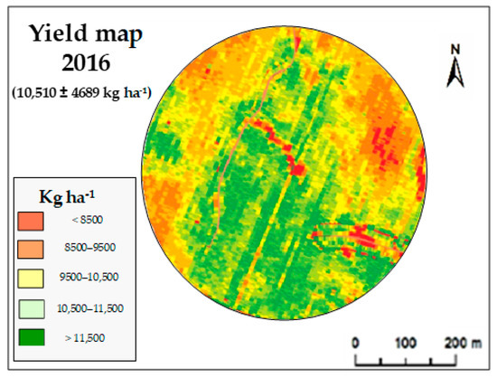
Figure 4.
Corn yield map of a “Eucalyptus” field in October 2016.
Figure 5 shows soil ECa maps at 0–0.5 m depth (a) and 0–1.0 m depth (b), with average values of, respectively, 12.71 ± 8.12 mS m−1 and 20.98 ± 23.08 mS m−1. Soil sampling points are referenced in these maps.
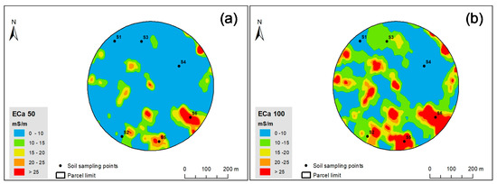
Figure 5.
Soil apparent electrical conductivity (ECa) maps of “Eucalyptus” field in April 2017: at 0–0.5 m (a) and 0–1.0 m (b).
The results of the soil analysis are shown in Table 2. It is a sandy soil (sand >90%) with low levels of organic matter and total N (both about 1%) and with acceptable levels of P2O5 (about 50 mg kg−1), poor performance in exchangeable cations, and high levels of Fe2+. Figure 5 shows that sampling points 5 and 6 correspond to areas with high ECa values, and, as indicated in Table 2, they are also the sampling points with higher values of soil silt and organic matter contents, showing a small gradient of soil fertility.
Table 2.
Soil characteristics of the “Eucalyptus” field at 0–0.30 m depth.
Figure 6 shows the altimetric map of “Eucalyptus” field, where a small elevation range (13–18 m) can be observed. This figure also shows the location of two SMC probes (P1 and P2) including one in the north of the field and another in the south.
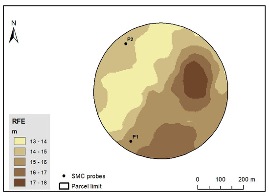
Figure 6.
Altimetric map of the “Eucalyptus” field. P1 and P2 are soil moisture content (SMC) probes.
Figure 7 shows eight NDVI maps of the “Eucalyptus” field including two for each month between June (after planting) and September (before harvesting).
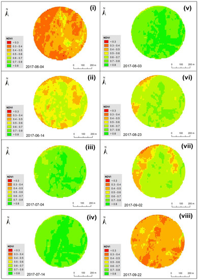
Figure 7.
Normalized difference vegetation index (NDVI) maps of the “Eucalyptus” field in different dates (maps (i)–(viii)), between June and September 2017.
The evolution of the NDVI reflects the evolution of the crop’s vegetative vigour. It increases from germination as the crop develops, reaching maximum values between mid-July (Figure 7(iv)) and early August (Figure 7(v)) and then decreasing until harvest (Figure 8). The pattern of the NDVI spatial variability over this period is as follows. The zones that, at the beginning of the vegetative cycle, reach high NDVI values (for example, in 14 June, Figure 7(ii)) are also those that, at the end of the vegetative cycle, are also the first to show a significant decrease in NDVI (for example, 23 August, Figure 7(vi) or in 2 September, Figure 7(vii)). As mentioned in material and methods, NDVI maps of 14 June (mean NDVI of 0.450 ± 0.055) and 23 August (mean NDVI of 0.621 ± 0.097) were used to redefine irrigation prescription maps.
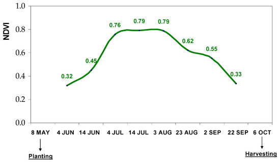
Figure 8.
Evolution of mean normalized difference vegetation index (NDVI) between June and September 2017.
Figure 9 shows the three management zones (MZ) identified in each of the three steps (left) and the corresponding maps converted into the pie slice format (right). In all maps, the “low class” represents areas with less potential (less fertility in HMZ 1, less vegetative vigour in HMZ 2 and 3), “high class” represent areas with greater potential (greater fertility in HMZ 1, greater vegetative vigour in HMZ 2 and 3) and “medium class” represents areas with an intermediate potential from the previous ones. These maps are tools to support precision crop management, which will always be conditioned by the objectives established in each specific phase. In this case study, the farmer’s main objective was to stimulate crop productivity in areas with less productive potential at the expense of applying greater amounts of water, which led to the establishment of the VRI maps presented in Figure 10 and implemented in 14 June (VRI 1), between 17 June and 22 August (VRI 2: 32 irrigation events) and between 24 August and 13 September (VRI 3: 9 irrigation events), as a result of SMC monitoring performed continuously by two capacitance probes. Five prescription classes were defined for the first year, but, in each VRI map, only three classes were used: (i) “standard” corresponds to the amount of irrigation that the farmer normally uses (present in all VRI maps), (ii) “+10%,” and (iii) “+20%,” respectively, 10% or 20% higher irrigation than the “standard” amount, corresponding to lower center pivot travel speed (classes used only in VRI maps 1 and 2 with the objective of stimulating the productivity of less fertile soils, areas with lower yield potential, and less vegetative vigour), (iv) “−10%” and (v) “−20%,” respectively, 10% or 20% less lower irrigation than the “standard” amount, corresponding to faster center pivot travel speed (classes used only in VRI map 3 with the objective of rationalizing the application of water in areas where the crop is in advanced stages of development). The area (as a percentage of the total area) that each prescription class represented in each VRI plan is presented in Table 3. The application of the data contained in Table 3 in Equations (2) and (3) indicate an increase of 5.5% in the irrigation amounts as a result of the implementation of this variable irrigation strategy when compared to a conventional and uniform prescription.
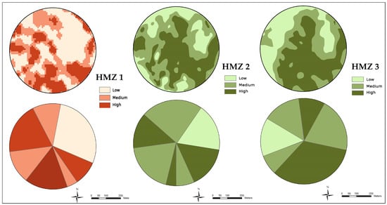
Figure 9.
Homogeneous management zones (HMZ) maps 1, 2, and 3 (left) and the correspondent maps converted into the pie slice format (right).
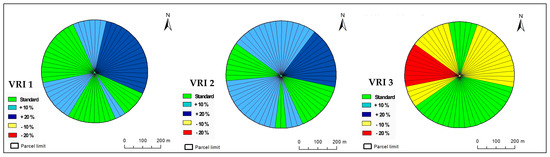
Figure 10.
Variable rate irrigation (VRI) maps 1, 2, and 3 implemented in the “Eucalyptus” field between 14 June and 13 September 2017.
Table 3.
Area (percentage of the total) that each prescription class represented in each variable rate irrigation (VRI) plan.
The evaluation of the impact of the variable irrigation strategy was also carried out in this first year in terms of crop productivity (total production and spatial variability). Figure 11 shows the corn yield map of the field in October 2017. In addition to the increase of 8% in the productivity (changed from 10,510 ± 4689 kg ha−1 in 2016 to 11,350 ± 4097 kg ha−1), there was also a decrease in spatial variability (CV = 36.1% in 2017, against 44.6% in 2016).
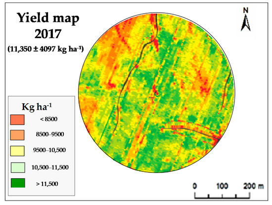
Figure 11.
Corn yield map of the “Eucalyptus” field in October 2017.
4. Discussion
VRI comes into play as an engineering solution to manage spatial allocation of water applied through irrigation, which is the most valuable input for agriculture across the world [5]. The prime drawbacks of VRI systems are high capital costs for implementation and management [13]. Most of the available center pivots, however, have control panels with a speed control module, meaning farmers can vary the irrigation across their fields to some extent at no extra cost, if it is needed [5]. Changing the pivot travel speed enables the establishment and management of individual pie shape zones where faster pivot travel results in less irrigation and slower travel speed results in increased irrigation at the selected pies [13]. Nevertheless, dynamic prescription maps are necessary because soil water content varies not only temporally, but also spatially, even in leveled fields [2]. The objective of this case study was to evaluate tools for definition of dynamic HMZ (ECa obtained by proximal sensor and NDVI obtained by remote sensing) and dynamic VRI maps to automatic center pivot travel speed control in corn. Delineating irrigation zones is the first step toward site-specific irrigation management [5]. It can even be said that it is not only the first, but also a fundamental step, since the quality of HMZ will influence the irrigation prescription maps. There are usually three paths used to survey variability and define HMZ [2,5]: (i) soil ECa measurements with proximal sensors (the starting point for variability), (ii) monitoring of vegetation indices based on satellite images, mainly NDVI (the dynamic crop evolution), and (iii) yield data (the final objective of the production process). However, despite similarities between the zones delineated by these three sources (as shown in this study), yield data has less potential because of its inconsistency, since yield is affected by the complex interaction of different factors, which is contrary to what happens with soil ECa [20], which shows a certain degree of temporal stability [21]. Additionally, Moral et al. [22] found that the temporal stability of soil ECa makes it a better proximal attribute for high resolution zone delineation. This study confirmed similar spatial patterns of ECa maps in both soil layers (0–0.5 m and 0–1.0 m depth), although with higher soil ECa values at greater depth (20.98 ± 23.08 mS m−1 at 1.0 m depth and 12.71 ± 8.12 mS m−1 at 0.5 m), which is due to the cumulative influence of the ECa measured by the sensor [23]. It is evident that the 1.0-m depth map allows a better stratification of the classes of ECa and, therefore, a greater potential for the definition of management zones, which is in line with other works [5].
The overlap of the ECa and altimetric maps shows that the lower values of ECa correspond to higher elevation zones of the field, seeming to indicate an inverse relationship between these two parameters, which is an aspect already demonstrated in other works [24,25]. According to Marques da Silva et al. [26], surface topography plays a significant role in influencing spatial ECa patterns. A higher soil electrical conductivity is observed in lower areas where soil moisture levels tend to be naturally higher at the end of spring (April) in Mediterranean climates. In view of this relationship, as suggested by O’Shaughnessy et al. [2], in this study, ECa and topographical information were combined to delineate initial HMZ. The initial proposal also included smart soil sampling, which is suggested by several studies [22]. However, the results (Table 2) showed reduced variability and some inconsistency, and cannot be used to explain the spatial variability of ECa, the vegetative vigour or the crop yield, and, therefore, were not included in the final HMZ calculation and definition algorithm.
Another aspect that is interesting to highlight and to which several authors draw attention [2,5] is the critical need to dynamically develop irrigation HMZ. This challenge is based on the fact that spatial arrangement of irrigation MZ may change during the growing season [2]. This dynamic adaptation over time must also be achieved in an accurate and inexpensive manner [5]. In our study, it was based on the mapping of NDVI at specific times with different purposes: (i) about 1 month after planting (14 June 2017) to stimulate the productivity of areas with less vegetative vigour, and (ii) about two weeks before harvest (22 August 2017) to rationalize the application of irrigation water in areas where the crop was in advanced stages of its vegetative cycle.
This was an exploratory case study in Portugal, financed by European funds (European Regional Development Fund, Project “PDR2020-101-FEADER-032167”). The objective was to develop and demonstrate a feasible and relatively affordable method for the creation of dynamic prescription maps needed to control site-specific variable irrigation in corn. The implementation of the “speed control” VRI technology can be carried out with a minimal learning curve and have a relatively low cost resulting in a quicker return on investment, when compared with other more complex solutions, namely the “zone control” systems s [2].
The results of this first year showed a positive trend in achieving the initial goal established by the farmer, reducing the spatial variability of corn productivity in this field (CV = 36.1% in 2017, against 44.6% in 2016). In addition, this field registered an increase of 8% in the corn productivity at the expense of an increase of 5.5% in the irrigation water amounts when compared to conventional and uniform prescription. Although these results can be viewed in the perspective of the natural inter-annual variability of crop yield as a result of climatic trends, the data clearly indicate an improvement in the irrigation water use efficiency (IWUE), which relates crop yield produced per unit of water supplied [27], and could lead the farmer to readjust his objectives. As part of the precision agriculture (PA) concept, the objectives are revaluated after the end of each crop cycle, and, thus, the farmer can focus on identifying possible structural causes (for example, soil compaction or poor drainage) that help to explain the historically marginal yields in some areas, where the amount of irrigation can be reduced [2] instead of increasing the amounts of irrigation water to compensate its lower productive potential. Within the scope of the PA, an approach that addresses the effect of the VRI strategy on crop productivity and the amount of irrigation water used, but also accounts for the costs associated with the technologies and technical support, will be important. For example, in this specific case, the initial cost of “speed control” VRI technology (approximately 3000 €, which can be added to existing moving irrigation systems) must be considered. Additionally, in the first year, the cost of soil ECa survey (approximately 40 € per ha) should be considered. Annually, a budget of around 1500 € should be considered for the services needed to obtain, process, and integrate all the information as well as capture the satellite images, obtain the respective indices (NDVI), and define and present the VRI maps.
This study demonstrates how a relatively simple solution for the implementation of VRI “speed control” could be designed and implemented, showing that PA techniques are ready to provide tangible results that may be of interest not only for researchers, but also for farmers. One of the advantages of the PA approach is that historical digital information can be stored and, subsequently, processed and used. For example, promising results have been reported by studies that have averaged yield data over years, eliminating the problem of temporal instability and providing more reliable HMZ [2]. Currently, the large-scale implementation of this or similar systems in the region, it will be essential to carry out a cost-benefit analysis to investigate and to select approaches that are economically (improved crop production) and environmentally (reduced amount of irrigation water) appropriate and acceptable to a producer and that can convince farmers and growers to adopt this strategy. Further works on various complex soils and climate conditions will be helpful for establishing a more general method of mapping irrigation prescription needed for application of VRI technology based on “speed control” or evolving to more complex and also more expensive systems, such as the “zone control.”
A limitation of this study is the unavailability of detailed records, indicating the amounts of irrigation water applied throughout the crop vegetative cycle, which makes it unfeasible to calculate the IWUE. Future studies, involving several years of implementation of VRI in different farms, with detailed records of productivity and also of the absolute amounts of applied water, will allow the calculation of the IWUE for both uniform and variable (VRI) irrigation strategies, which will serve as the basis for the promotion and demonstration of these precision agriculture technologies.
5. Conclusions
Climate change has direct consequences on water availability, requiring the development of strategies to optimize its use. Conventional irrigation systems are based on the application of a homogeneous input over the field, considered as a uniform spatial unit. However, frequently, fields can have spatial heterogeneity of soil characteristics, topography, microclimate, and crop development. Improving the efficiency of water use is one of the main challenges currently facing farm managers. The large area of center pivot-irrigated crops in Portugal (over 200,000 hectares) and in the world (over eight million hectares) requires a differentiated response to irrigation management. VRI is a novel engineering solution to manage spatial allocation of irrigation water.
The objective of this case study was to evaluate tools for delineating dynamic HMZ and defining dynamic VRI maps needed to automate center pivot travel speed control in corn. The results of this first year showed a positive trend in achieving the initial goal established by the farmer, reducing the spatial variability and increasing corn productivity in this field, at the expense of a light increase in irrigation water amounts. ECa and topographical information obtained by on-the-go sensors and NDVI obtained by remote sensing proved to be effective in the definition of dynamic management zones and appealing because of the ease with which they can be collected at a field-scale. A contribution to more reliable HMZ may result from the application of the PA concept with the integration of yield maps of several years, averaged to reduce their temporal instability.
This relatively simple approach is fairly inexpensive for the farmer and can be implemented on a large scale, which represents an important and sustainable contribution to improved water use efficiency in Mediterranean agriculture, especially in the current scenario of global warming and reduction of the available water for agriculture.
Author Contributions
Conceptualization, J.S., S.G., J.P., and J.N. Methodology, J.S., S.S., J.M.d.S., L.P., F.M., R.C.-C., S.G., J.P., and J.N. Software, J.S., F.M., R.C.-C., and J.N. Validation, J.S., S.S., S.G., J.P., and J.N. Formal analysis, J.S., S.S., and J.N. Investigation, J.S., S.G., J.P., and J.N. Resources, J.S., S.S., J.M.d.S., L.P., F.M., R.C.-C., S.G., J.P., and J.N. Data curation, J.S., S.G., and J.N. Writing, J.S. and J.N. Writing—review and editing, J.S. and S.S. Visualization, J.S. and S.S. Supervision, J.S., S.S., and J.N. Project administration, J.S. and J.N. Funding acquisition, J.S. and J.N. All authors have read and agreed to the published version of the manuscript.
Funding
This work was funded by the project PDR2020−101-FEADER-032167 “Regadio de Precisão” (“Programa 1.0.1-Grupos Operacionais”).
Conflicts of Interest
The authors declare no conflict of interest.
References
- Baptista, V.B.D.S.; Córcoles, J.I.; Colombo, A.; Moreno, M.A. Feasibility of the use of variable speed drives in center pivot systems installed in plots with variable topography. Water 2019, 11, 2192. [Google Scholar] [CrossRef]
- O’Shaughnessy, S.A.; Evett, S.R.; Colaizzi, P.D.; Andrade, M.A.; Marek, T.H.; Heeren, D.M.; Lamm, F.R.; LaRue, J.L. Identifying advantages and disadvantages of variable rate irrigation: An updated review. Appl. Eng. Agric. 2019, 35, 837–852. [Google Scholar] [CrossRef]
- Ortuani, B.; Facchi, A.; Mayer, A.; Bianchi, D.; Bianchi, A.; Brancadoro, L. Assessing the effectiveness of variable-rate drip irrigation on water use efficiency in a vineyard in northern Italy. Water 2019, 11, 1964. [Google Scholar] [CrossRef]
- Zhang, X.; Chen, S.; Sun, H.; Wang, Y.; Shao, L. Water use efficiency and associated traits in winter wheat cultivars n the north China plain. Agr. Water Manage. 2010, 97, 1117–1125. [Google Scholar] [CrossRef]
- Haghverdi, A.; Leib, B.G.; Washington-Allen, R.A.; Ayers, P.D.; Buschermohle, M.J. Perspectives on delineating management zones for variable rate irrigation. Comput. Electron. Agric. 2015, 117, 154–167. [Google Scholar] [CrossRef]
- Torres-Sánchez, R.; Navarro-Hellin, H.; Guillamon-Frutos, A.; San-Segundo, R.; Ruiz-Abellón, M.D.C.; Domingo, R. A decision support system for irrigation management: Analysis and implementation of different learning techniques. Water 2020, 12, 548. [Google Scholar] [CrossRef]
- West, G.H.; Kovacs, K. Addressing groundwater declines with precision agriculture: An economic comparison of monitoring methods for variable-rate irrigation. Water 2017, 9, 28. [Google Scholar] [CrossRef]
- Monaghan, J.M.; Daccache, A.; Vickers, L.H.; Hess, T.M.; Weatherhead, E.K.; Grove, I.G.; Knox, J.W. More ‘Crop Per Drop’: Constraints and Opportunities for Precision Irrigation in European Agriculture. J. Sci. Food Agric. 2013, 93, 977–980. [Google Scholar] [CrossRef]
- Yari, A.; Madramootoo, C.A.; Woods, S.A.; Adamchuk, V. Performance evaluation of constant versus variable rate irrigation. Irrig. Drain. 2017, 66, 501–509. [Google Scholar] [CrossRef]
- Longchamps, L.; Khosla, R.; Reich, R.; Gui, D. Spatial and temporal variability of soil water content in leveled fields. Soil Sci. Soc. Am. J. 2015, 79, 1446–1454. [Google Scholar] [CrossRef]
- Zhao, W.; Li, J.; Yang, R. Crop yield and water productivity responses in management zones for variable-rate irrigation based on available soil water holding capacity. Trans. ASABE 2017, 60, 1659–1667. [Google Scholar] [CrossRef]
- Castrignanò, A.; Buttafuoco, G.; Quarto, R.; Vitti, C.; Langella, G.; Terribile, F.; Venezia, A. A combined approach of sensor data fusion and multivariate geostatistics for delineation of homogeneous zones in an agricultural field. Sensors 2017, 17, 2794. [Google Scholar] [CrossRef] [PubMed]
- Evans, R.G.; LaRue, J.; Stone, K.C.; King, B.A. Adoption of site-specific variable rate sprinkler irrigation systems. Irrig. Sci. 2013, 31, 871–887. [Google Scholar] [CrossRef]
- FAO. World Reference Base for Soil Resources; Food and Agriculture Organization of the United Nations, World Soil Resources Reports No. 103; IUSS Working Group WRB: Rome, Italy, 2006. [Google Scholar]
- AOAC. AOAC Official Methods of Analysis of AOAC International, 18th ed.; AOAC International: Arlington, VA, USA, 2005. [Google Scholar]
- Gao, B.-C. NDWI—A normalized difference water index for remote sensing of vegetation liquid water from space. Remote. Sens. Environ. 1996, 58, 257–266. [Google Scholar] [CrossRef]
- Höppner, F.; Klawonn, F.; Kruse, R.; Runkler, T.A. Fuzzy Cluster Analysis; Wiley: Chichester, UK, 1999. [Google Scholar]
- Fridgen, J.J.; Kitchen, N.R.; Sudduth, K.A.; Drummond, S.T.; Wiebold, W.J.; Fraisse, C.W. Management zone analyst (MZA): Software for subfield management zone delineation. Agron. J. 2004, 96, 100–108. [Google Scholar] [CrossRef]
- Tagarakis, A.; Liakos, V.; Fountas, S.; Koundouras, S.; Gemtos, T.A. Management zones delineation using fuzzy clustering techniques in grapevines. Precis. Agric. 2013, 14, 18–39. [Google Scholar] [CrossRef]
- Corwin, D.L.; Lesch, S.M.; Segal, E.; Skaggs, T.H.; Bradford, S.A. Comparison of sampling strategies for characterizing spatial variability with apparent soil electrical conductivity directed soil sampling. J. Environ. Eng. Geophys. 2010, 15, 147–162. [Google Scholar] [CrossRef]
- Heil, K.; Schmidhalter, U. Improved evaluation of field experiments by accounting for inherent soil variability. Eur. J. Agron. 2017, 89, 1–15. [Google Scholar] [CrossRef]
- Moral, F.J.; Terrón, J.; Da Silva, J.M. Delineation of management zones using mobile measurements of soil apparent electrical conductivity and multivariate geostatistical techniques. Soil Tillage Res. 2010, 106, 335–343. [Google Scholar] [CrossRef]
- Serrano, J.M.; Shahidian, S.; Da Silva, J.R.M. Spatial variability and temporal stability of apparent soil electrical conductivity in a Mediterranean pasture. Precis. Agric. 2017, 18, 245–263. [Google Scholar] [CrossRef]
- Tarr, A.B.; Moore, K.J.; Bullock, D.G.; Dixon, P.M.; Burras, C.L. Improving map accuracy of soil variables using soil electrical conductivity as a covariate. Precis. Agric. 2005, 6, 255–270. [Google Scholar] [CrossRef]
- Serrano, J.M.; Peça, J.O.; Da Silva, J.R.M.; Shaidian, S. Mapping soil and pasture variability with an electromagnetic induction sensor. Comput. Electron. Agric. 2010, 73, 7–16. [Google Scholar] [CrossRef]
- Da Silva, J.R.M.; Peça, J.; Serrano, J.M.; De Carvalho, M.; Palma, P.M. Evaluation of spatial and temporal variability of pasture based on topography and the quality of the rainy season. Precis. Agric. 2008, 9, 209–229. [Google Scholar] [CrossRef][Green Version]
- Chai, Q.; Gan, Y.; Zhao, C.; Xu, H.L.; Waskom, R.M.; Niu, Y.; Siddique, K.H.M. Regulated deficit irrigation for crop production under drought stress. A review. Agron. Sustain. Dev. 2016, 36, 3. [Google Scholar] [CrossRef]


Publisher’s Note: MDPI stays neutral with regard to jurisdictional claims in published maps and institutional affiliations. |
© 2020 by the authors. Licensee MDPI, Basel, Switzerland. This article is an open access article distributed under the terms and conditions of the Creative Commons Attribution (CC BY) license (http://creativecommons.org/licenses/by/4.0/).