Article

Effects of Two-Phase Flow of Water and Air on Shallow Slope Failures Induced by Rainfall: Insights from Slope Stability Assessment at a Regional Scale

1
School of Urban and Environmental Engineering, Ulsan National Institute of Science and Technology, 50 UNIST-gil, Ulju-gun, Ulsan 44919, Korea
2
Department of Civil and Environmental Engineering, Hankyong National University, 327 Jungang-ro, Anseong-si, Gyeonggi 17579, Korea
3
Department of Civil Engineering, Kumoh National Institute of Technology, 61 Daehak-ro, Gumi-si, Gyeongbuk 39177, Korea
*
Author to whom correspondence should be addressed.
Water 2020, 12(3), 812; https://doi.org/10.3390/w12030812
Submission received: 17 February 2020 / Revised: 10 March 2020 / Accepted: 10 March 2020 / Published: 14 March 2020
(This article belongs to the Section Hydrology)

Abstract

:
Over 160 shallow landslides resulted from heavy rainfall that occurred in 26–27 July 2011 at Umyeon Mountain, Seoul, South Korea. To accurately reflect the fluid flow mechanism in the void spaces of soils, we considered the two-phase flow of water and air for rainfall infiltration analysis using available historical rainfall data, topographic maps, and geotechnical/hydrological properties. Variations in pore water and air pressure from the infiltration analysis are used for slope stability assessment. By comparing the results from numerical models applying single- and two-phase flow models, we observed that air flow changes the rate of increase in pore water pressure, influencing the safety factor on slopes with a low infiltration capacity, where ponding is more likely to occur during heavy rainfall. Finally, several slope failure assessments were conducted to evaluate the usefulness of using the two-phase flow model in forecasting slope stability in conditions of increased rainfall sums. We observed that the two-phase flow model reduces the tendency of over-prediction compared to the single-phase model. The results from the two-phase flow model revealed good agreement with actual landslide events.

1. Introduction

Rainfall-induced landslides have caused many human casualties and severe property damage worldwide [1,2]. The initiation of rainfall-induced landslides is affected by various factors, such as the material properties of soil, topographic features, geological and hydrological characteristics, slope surface cover, and vegetation [3,4]. Slope failures are caused by not only the infiltration of water into the soil of slopes during heavy rainfall but also the groundwater rise or the lateral water flow in the underground of slopes after precipitation, triggering buoyancy forces owing to changes in water pressure near the slope foot [5,6,7,8]. During the rainfall infiltration, the increase in water content causes an increase in the unit weight of the soil [9,10], and the loss of matric suction as wetting bands progress into the slope decreases its shear strength and effective stress [11,12].
Although numerous empirically based approaches have been widely applied to large areas using simple methods, deterministic physics-based approaches are preferable for a better understanding of the mechanisms of shallow landslides [13]. Numerous physically based studies have investigated infiltration behavior during rainfall using various approaches: (1) Adopting assumptions for simplification to solve the differential equation of Richards [14] by applying a single-phase fluid (water) flow [3,10,15,16]; (2) assuming that the air pressure in the void spaces of an unsaturated soil slope is equal to the atmospheric pressure [9,17,18]; (3) applying a two-phase fluid (water and air) flow [19,20,21,22,23]; and (4) considering hydraulic hysteresis, including the effects of capillarity and/or air entrapment, reflecting different hydraulic states under wetting and drying conditions [24,25]. Such physically based numerical studies have mainly been applied at slope or watershed scales.
Slope stability assessments at a regional or local scale are required to simulate landslide events. Simoni et al. [26] simulated shallow landslides using GEOtop-FS [27], which models subsurface flow based on the numerically integrated 3D Richards equation and assesses slope stability depending on a specified topography. Chen et al. [28] utilized Scoops3D [29] to evaluate landslide events in Hualien, Taiwan. However, such simulation in a 3D scheme incurs an excessive amount of computation [16]. Park et al. [30], Jeong et al. [15], Tran et al. [16], and Tran et al. [31] assessed the slope failures that occurred at Umyeon Mountain in Seoul, South Korea in 2011 using SEEP/W and SLOPE/W [32], TRIGRS [33], TiVaSS [34], and Scoops3D [29], respectively. However, air flow was not considered. As the ground consists of materials in three phases (soil particles, water, and air), it is necessary to consider two-phase flow to interpret rainfall infiltration accurately [11]. Several experiments and interpretations have reported that the air flow generated during infiltration changes the rate of the infiltrating water, affecting the safety factor. Therefore, it is apparent that the effect of air on the subsurface flow of fluids is relevant and should be included in infiltration analysis [21,22,35,36].
To efficiently utilize computing resources with application of a two-phase flow model based on numerical methods at a regional scale, each slope based on the geographic information system (GIS)-based topography of Umyeon Mountain located in Seoul, South Korea was simplified to be an infinite slope in a two-dimensional (2D) domain. We then applied the two-phase flow model to the infinite slopes for simulations of the rainfall-induced slope failure. Based on the variations in pore air and water pressures obtained from the simulation of rainfall infiltration, slope failure analyses were performed to compute safety factors at each infinite slope model. The minimum safety factor of elements in the infinite slope was considered to be a safety factor at the corresponding GIS-based topography cell. We evaluated the performance of the analysis for slope failure assessments applying the two-phase flow model. This study is concerned with (1) the investigation of the effects of air flow and pressure on infiltration behavior by comparing the variations in the pore water pressure predicted by the single-phase flow and two-phase flow models, (2) interpretations of the influence of air flow and pressure on safety factors during heavy rain, (3) comparison of the landslide susceptibility maps that were obtained by applying the single-phase flow and two-phase flow models, and (4) assessments of the applicability of single-phase flow and two-phase flow models by comparing areas that are predicted as unstable with the locations of actual landslide events.

2. Materials and Methods

2.1. Study Area

Umyeon Mountain is in Seoul, South Korea, at 37°27′00″–37°29′55″ N and 126°59′02″–127°01′41″ E. It has an area of approximately 5 km2. Figure 1 shows the elevation distribution of the study area based on 1:5000 digital maps produced by the National Geographic Information Institute of Korea [37] using the airborne laser terrain mapping system. The highest elevation is 295 m above sea level. The area around Umyeon Mountain consists mainly of Pre-Cambrian banded biotite gneiss and granitic gneiss [38]. According to Jeong et al. [15], the bedrock is primarily intensely weathered and substantially fractured plagioclase, quartz, biotite, feldspar, and amphibole. Umyeon Mountain is completely surrounded by urban development.
Approximately 160 catastrophic shallow landslides occurred in this area owing to heavy rain on 26–27 July 2011, with a cumulative total of 470 mm over the two days [39]. Debris flows that resulted from slope failures occurred along 20 watersheds from 7:00 to 9:00 local time on 27 July 2011, resulting in 16 deaths and severe structural damage to 10 buildings. The economic loss caused by the landslides was approximately 15 million US dollars [30].
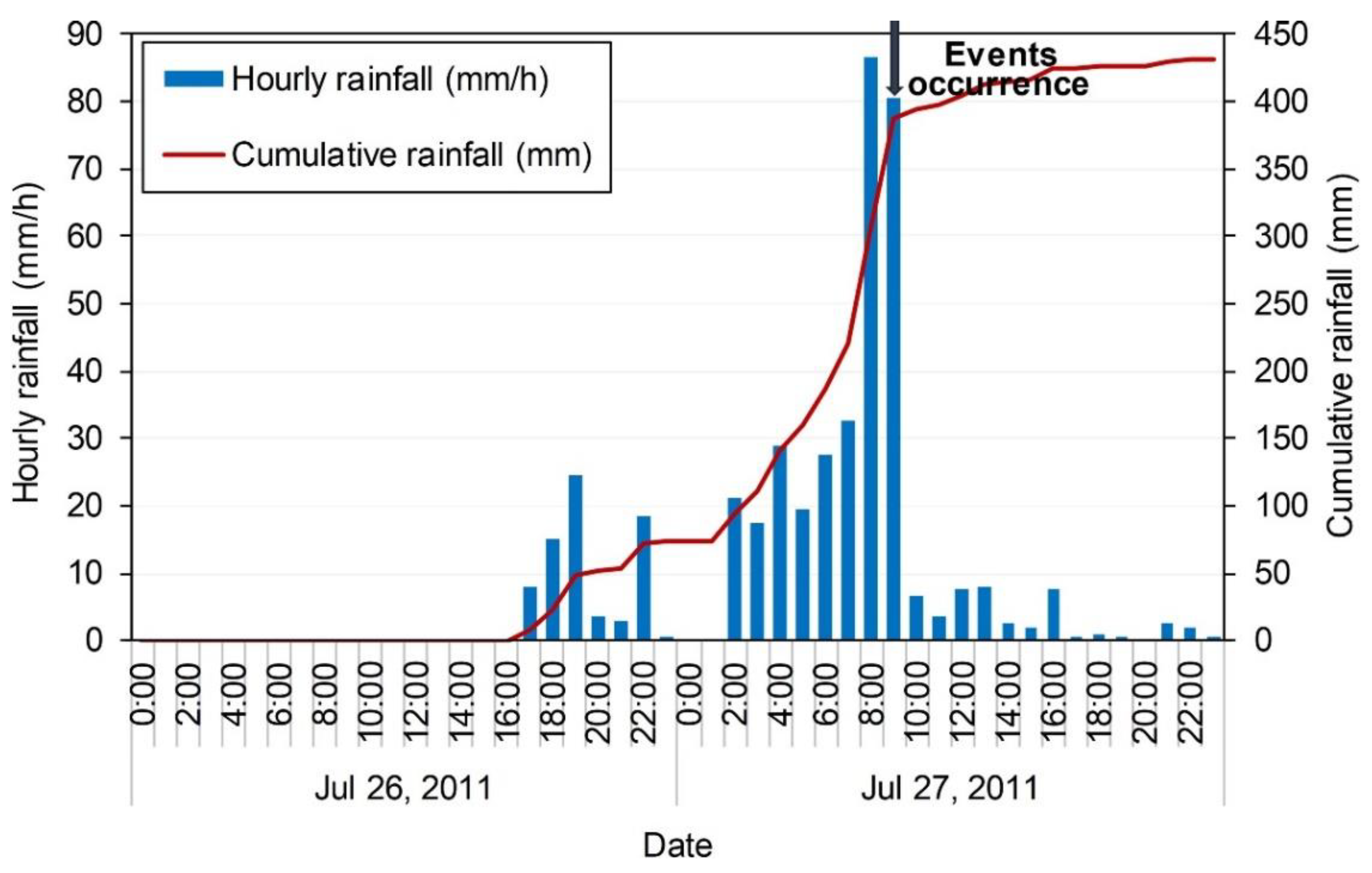
The weather station closest to Umyeon Mountain is Namhyun station. It is approximately 2 km away and is included in the automatic warning system (AWS) operated by the Korea Meteorological Administration (KMA) [40]. A precipitation of 1120 mm (i.e., approximately 55% of the normal annual precipitation in 2011) occurred in the area of Umyeon Mountain over July 2011. A maximum hourly rainfall of 114 mm/h occurred from 07:44 to 08:44 on 27 July. Figure 2 shows the time series for hourly and cumulative rainfall recorded at the Namhyun station during the two days from 26 July to 27 July 2011. Continuous rainfall of 320 mm occurred during the 8 h prior to the landslide events with strong rainfall intensities (higher than 17.5 mm/h). During the 2 h immediately prior to the landslide events, the rainfall attained 167 mm (i.e., 43% of the cumulative rainfall during the two days from 26 July to 27 July 2011).

2.2. Data

2.2.1. Landslide Inventories and Spatial Data

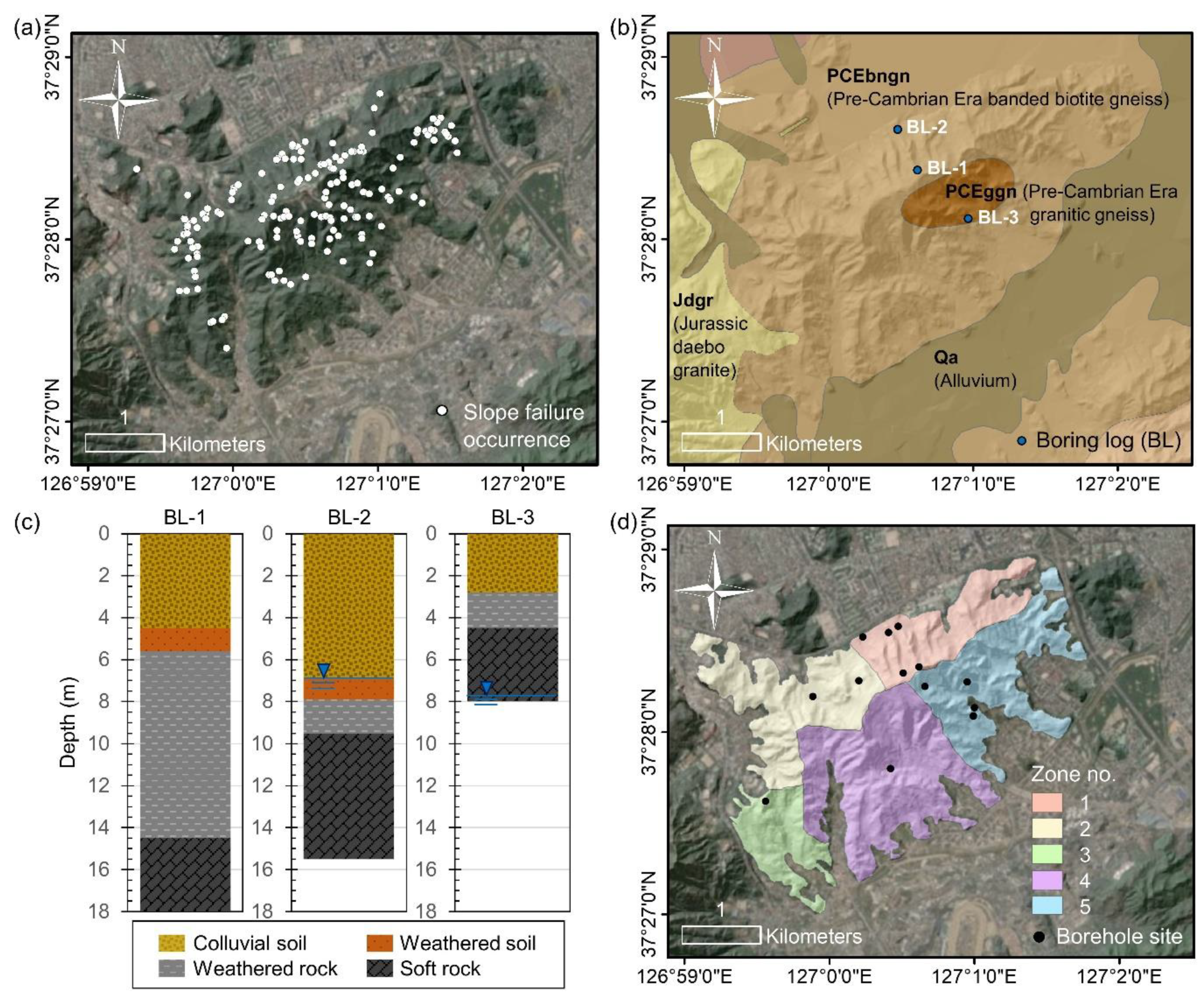
Landslide inventories of information on slope failures are important for validating the applicability of slope stability assessments. We compared satellite images with a resolution of 5 m and aerial photographs with a resolution of 25 cm to map the slope failure sites extracted from the study area before and after the 2011 landslides. A total of 161 slope failure initiation sites were constructed in a GIS format (Figure 3a). We also assessed the suitability of the available landslide inventories by comparing them with field survey-based data [41].
GIS-based topographic information is also required for slope stability assessments at a regional scale. We used a digital elevation model (DEM) with a 10 m-cell size computed from 1:5000 digital maps produced by the National Geographic Information Institute of Korea [37] (see Figure 1).

2.2.2. Material Properties

Representative geological units in the area of Umyeon Mountain are PCEbngn (Pre-Cambrian Era banded biotite gneiss), PCEggn (Pre-Cambrian Era granitic gneiss), and Jdgr (Jurassic daebo granite), as shown in Figure 3b. Pre-CambrianEra banded biotite gneiss, the lowest strata, is widely distributed in the study area, and Pre-Cambrian Era granitic gneiss and Jurassic daebo granite are distributed in relatively small areas near the top and western part of Umyeon Mountain, respectively. Jurassic daebo granite formed in the Mesozoic Jurassic period and has intruded into Pre-Cambrian Era banded biotite gneiss. The rocks that form the bedrock are slightly weathered or moderately weathered, and the rocks at the top of the mountain are more weathered than those at the bottom of the mountain [41]. Colluvium underlain by weathered soils is distributed in the entire area of Umyeon Mountain with unconformity, composed of loose silty sand mixed with gravel [42]. Figure 3c shows the boring logs and groundwater levels obtained from three different sites (BL-1, BL-2, and BL-3 shown in Figure 3b). The groundwater tables were distributed underneath the colluvium layer. The Korean Geotechnical Society [42] reported that most of the slope failures occurred at shallow depths with a range from 0.5 to 2 m and that depths of colluvium near the slope failure sites ranged from 0.3 to 3 m. We assumed that slope failure could occur in the colluvium layer with constant geotechnical properties. Infiltration and slope stability analyses were then performed with a focus more on the geotechnical characteristics than on the geological structure.
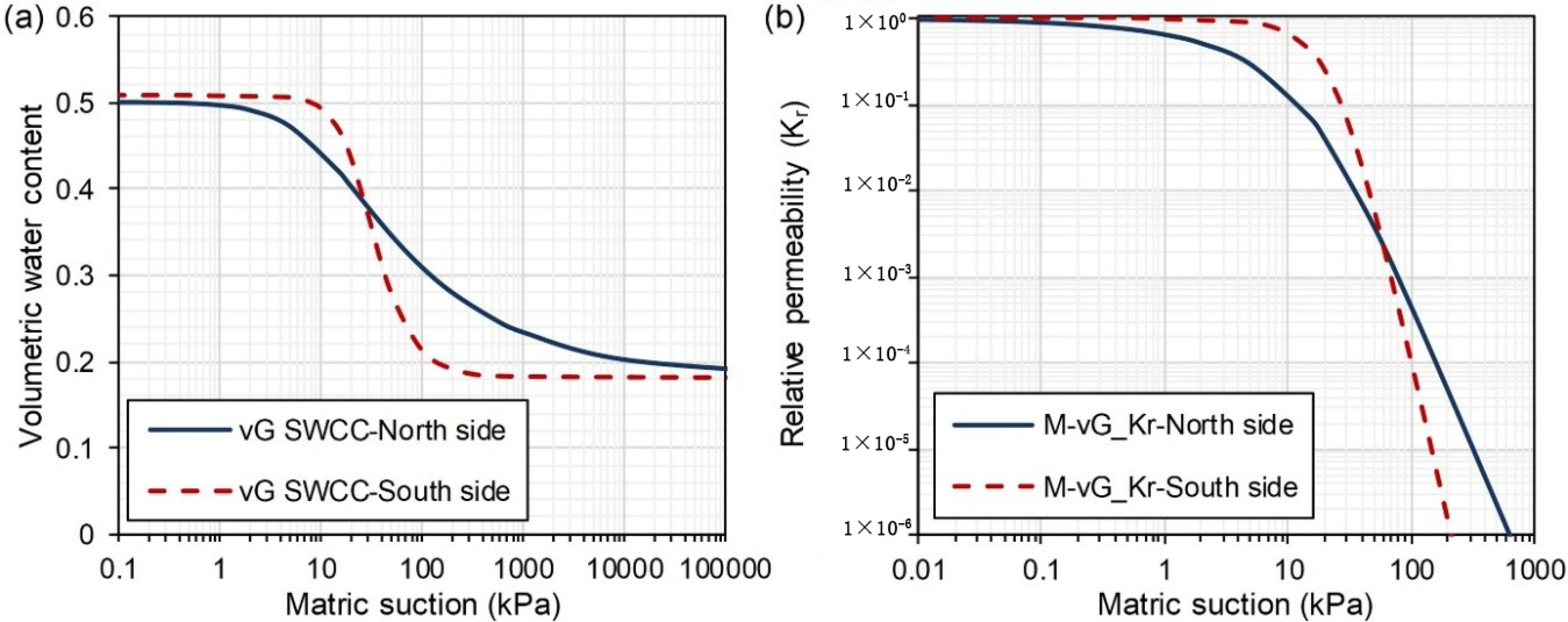
The Seoul Metropolitan Government [41] carried out detailed geotechnical field investigations at Umyeon Mountain by drilling 58 boreholes. Park et al. [30] used the geotechnical properties available from 13 boreholes and divided Umyeon Mountain into five zones based on the distribution of boreholes, geotechnical properties, and watersheds (Figure 3b). The cohesion, friction angle, and saturated hydraulic conductivity at borehole sites in zone 1 were in the ranges of 8.4–11.9 kPa with an average of 9.6 kPa, 24.8–26° with an average of 25.3°, and 6.67 × 10 6 8.08 × 10 6 m/s with an average of 7.15 × 10 6 m/s, respectively, and those at boreholes in zone 5 were in the ranges of 5.1–7.5 kPa with an average of 6.3 kPa, 27.6–30.3° with an average of 28.2°, and 2.08 × 10 6 4.45 × 10 6 m/s with an average of 3.69 × 10 6 m/s, respectively. Considering that the variations of them were not large and that simplification is required for simulations at a regional scale, we determined that the zones, categorized in Park et al. [30], could be appropriately applied in this study. Table 1 summarizes the soil properties (internal friction angle, cohesion, total/dry unit weight of soil, and saturated hydraulic conductivity) obtained from Park et al. [30] and the soil-water characteristics (i.e., soil-water characteristic curve (SWCC) [43] coefficients) obtained from the Seoul Metropolitan Government [41] in which the pressure plate method (GTCS) [44] and the filter paper method were applied. The representative soil properties are determined as the average values of the boreholes located in each zone. We applied two van Genuchten SWCCs, generally used in numerical methods, to the north side (zones 1 and 2) and south side (zones 3, 4, and 5) of Umyeon Mountain (Figure 4a). Figure 4b shows the Mualem–van Genuchten relative permeability curves [43] applied to the north and south areas in this study. The material properties of water and air applied to the infiltration analysis are presented in Table 2.

2.3. Methods

2.3.1. Rainfall Infiltration Analysis

We used FLAC 2D Ver. 7.0 [46] to apply the two-phase flow of water and air for the infiltration analysis of unsaturated soil slopes. This simulates the flow of two immiscible fluids in a porous medium. The pore spaces are assumed to be completely filled with the two fluids. In unsaturated soils, water and air can be substituted for the wetting fluid ( w ) and non-wetting fluid ( g ), respectively. van Genuchten [43] proposed Equation (1), which describes a relationship between effective saturation ( S e ) and matric suction ( ψ = non-wetting fluid pressure ( P g )—wetting fluid pressure ( P w )) as follows:
S e = [ ( ψ / P 0 ) 1 1 a + 1 ] a = S w S w r 1 S w r ,
where Sw is the actual saturation of the wetting fluid, and S w r is the residual saturation.
Darcy’s law allows calculation of how the wetting and non-wetting fluids are transported in the two-phase flow option. Equations (2) and (3) represent the velocities of the wetting and non-wetting fluids ( q i w and q i g ), respectively:
q i w = k i j w k r w x j ( P w ρ w g k x k ) ,
q i g = k i j w μ w μ g k r g x j ( P g ρ g g k x k ) ,
where k i j w is the saturated mobility coefficient ( = k s / ( g ρ w ) ), k s is the saturated hydraulic conductivity, g is the gravitational acceleration, ρ w is the density of the wetting fluid, k r is the relative permeability, μ w   /   μ g is the viscosity ratio between the wetting and non-wetting fluids, and ρ g is the density of the non-wetting fluid.
The relative permeability of a wetting fluid is required to calculate the unsaturated hydraulic conductivity. van Genuchten [43] proposed the relative permeability ( k r w ) based on the capillary model of Mualem [47] (Equation (4)). Lenhard and Parker [48] calculated the relative permeability of a non-wetting fluid ( k r g ), expressed as in Equation (5):
k r w = ( S e ) b { 1 [ 1 ( S e ) 1 a ] a } 2 ,
k r g = ( 1 S e ) c [ 1 ( S e ) 1 a ] 2 a ,
where b and c are constants. Both b and c are equal to 0.5 for water and air [11].
Equations (6) and (7) are the balance equations for the wetting and non-wetting fluids, respectively. These equations can be derived by combining the fluid balance laws with the fluid constitutive laws for the two fluids:
n [ S w K w P w t + S w t ] = [ q i w x i + S w ε t ] ,
n [ S g K g P g t + S g t ] = [ q i g x i + S g ε t ] ,
where n is the porosity, K is the fluid bulk modulus, t is the time, and ε is the volumetric strain.
The balance of momentum is described as in Equation (8):
σ i j x j + ρ g i = ρ d u i ˙ d t ,
where σ is the total stress, ρ is the bulk density, and u ˙ is the velocity of a soil particle.
The bulk density is described by Equation (9) for unsaturated soil conditions:
ρ = ρ d + n ( S w ρ w + S g ρ g ) ,
where ρ d is the dry density of soil.
We used Bishop’s effective stress [49] to analyze the failure of unsaturated soil in the Mohr–Coulomb constitutive model. Equation (10) presents the yield criterion of the Mohr–Coulomb constitutive model. Bishop’s effective stress ( σ b ) is expressed by Equation (11) as below:
τ max = σ b tan ϕ + c ,
σ b = ( σ P g ) + χ ( P g P w ) ,
where τ max is the shear strength, ϕ is the effective friction angle, c is the effective cohesion, and χ is the matric suction coefficient that varies from zero (i.e., dry conditions) to one (i.e., fully saturated conditions).
The degree of saturation can be approximately substituted for the matric suction coefficient [11,19,50,51,52]. Equation (12) was derived from Equation (11) by substituting the degree of saturation for χ . Equation (10) is then expressed as Equation (13):
σ b = σ ( S w P w + S g P g ) ,
τ max = [ σ ( S w P w + S g P g ) ] tan ϕ + c ,
where S w P w + S g P g is the pore fluid pressure.
The two-phase flow model is composed of the fluid flow and mechanical loops. The fluid flow loop computes fluid flows based on pressure gradients and variations in saturation and pore water and air pressures induced by unbalanced flows, utilizing from Equation (2) to Equation (7). The mechanical loop computes total stress, which depends on the coordinates, velocities, and pore pressure generation induced by mechanical volume strain, utilizing from Equation (8) to Equation (13). The stress state from the mechanical loop is used for the next time step of the fluid flow loop.

2.3.2. Slope Stability Analysis

The infinite slope analysis method can be used to interpret rainfall-induced shallow slope failure in Korea. This is because the failure surface is generally parallel to the slope surface in this region [3]. We applied the limit equilibrium method to the infinite slope. The safety factor of the infinite slope ( F s ) can be expressed as in Equation (14), given the Mohr–Coulomb failure criterion (Equations (10) and (13)) and Bishop’s effective stress (Equations (11) and (12)):
F s = τ f τ m = σ b tan ϕ + c W sin β cos β = [ W cos 2 β ( S w P w + S g P g ) ] tan ϕ + c W sin β cos β ,
where τ f is the shear strength of the soil, τ m is the shear stress on the failure surface, β is the slope angle, and W is the weight of a soil slice.
The total unit weight of soil ( W ) depends on variations in saturation caused by rainfall infiltration. To consider an increase in the unit weight of soil during rainfall, the weight of a soil slice per unit area above a potential failure surface can be described as in Equation (15):
W = 0 z w γ t d z = 0 z w [ γ d + n S w ( z ) γ w ] d z ,
where z w . is the depth from the slope surface to the potential failure surface, γ t is the total unit weight of soil, γ d is the dry unit weight of soil, γ w is the unit weight of water, and S w ( z ) is the saturation, which depends on depth.

2.3.3. Slope Geometry and Boundary/Initial Conditions

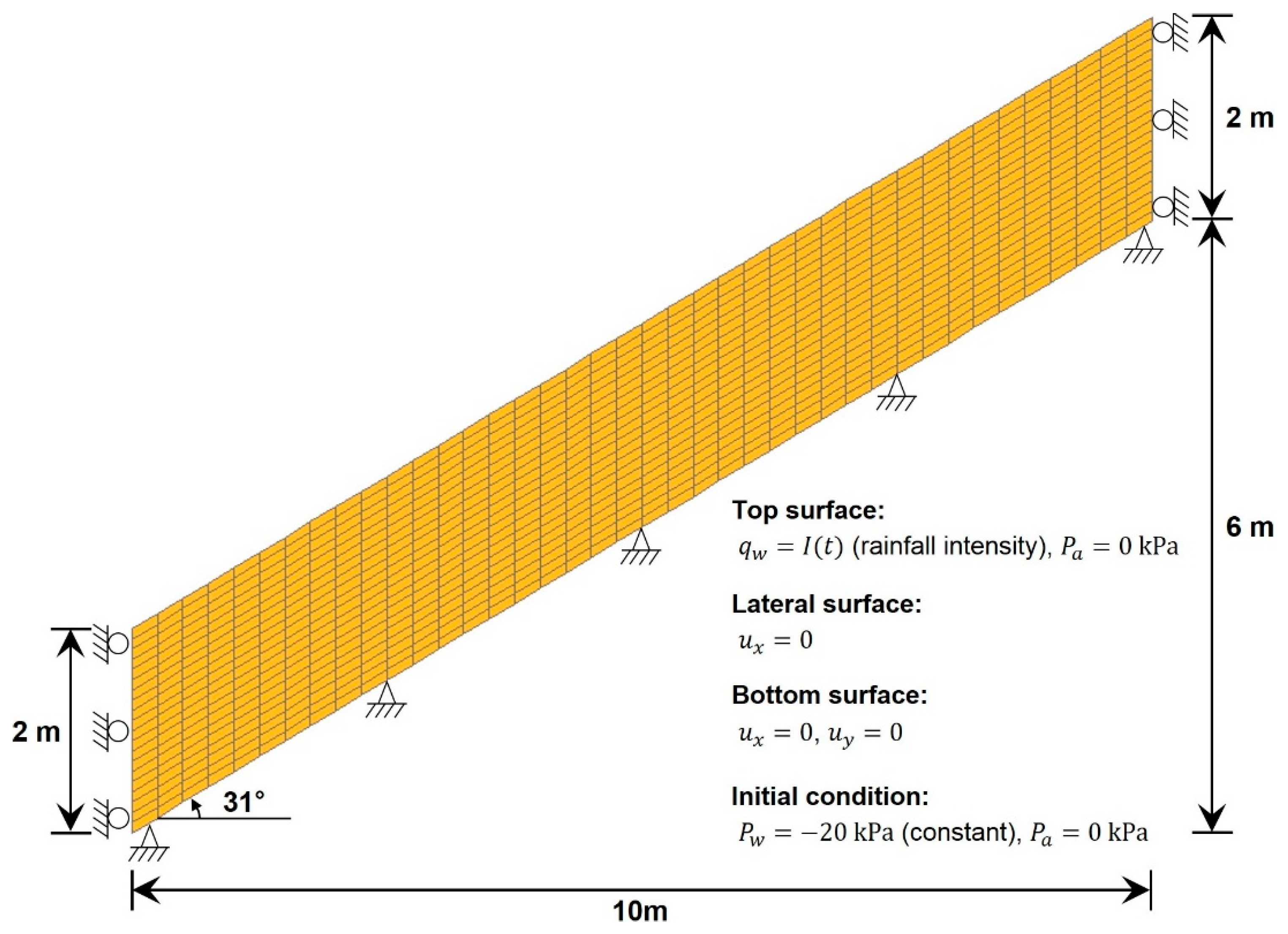
In Korea, the depth at which shallow slope failure surfaces are present generally ranges from 1 to 3 m [53], and such failure surfaces are parallel to the ground surface. Therefore, to assess slope failure, Park et al. [30] assumed a uniform soil depth of 2 m for Umyeon Mountain by considering an investigation of the distribution of soil depths by the Korean Geotechnical Korean Geotechnical Society [42]. We also modeled 2D infinite slopes with a uniform soil depth of 2 m and a length of 10 m, and we assumed the ground to be isotropic and homogeneous considering the engineering soil properties summarized in Table 1. Figure 5 illustrates an example of an infinite slope model with an angle of 31°, which is approximately equal to the mean slope angle of the slope failure sites in the study area (i.e., 31.2°). We applied the two-phase flow model for simulating rainfall infiltration to the independent infinite slope models, where slope angles were considered based on different cells of the GIS-based slope raster in the study area. Variations in pore water and air pressures ( P w and P a , respectively) and saturations with the time step could then be computed at the infinite slopes for 17 h during rainfall. The slope stability on the infinite slopes for the 17 h was calculated by applying the variations in P w , P a , and saturations computed from the two-phase flow model to Equation (14). Finally, we determined the safety factor of each cell of the GIS-based topography in the study area to be the minimum safety factor of the corresponding infinite slope model.
Water flux was set as equal to the hourly rainfall shown in Figure 2 and was applied at the ground surface as a boundary condition. The bottom surface was set to be completely constrained, at which displacements in both horizontal and vertical directions were fixed, and vertical fluid flows were unaccepted. Displacements in the horizontal direction were fixed at the left and right sides. The slope surface was subjected to the atmospheric boundary conditions. We set the initial P a on the slope as equal to atmospheric pressure. The other boundaries were assumed to be airtight. The P a applied in the single-phase flow option was set to zero.
The matric suction measured in the study area during a rainfall season in 2012 was maintained at 10–20 kPa prior to rainfall [41]. Therefore, we set the initial slope conditions to be steady-state with an initial P w of −20 kPa (a constant value by depth). The initial P w . can be set as constant near the surface grounds where the depth of the groundwater table is known to be deep [3,11].

2.3.4. Performance Evaluation of Slope Stability Assessment

To evaluate the quantitative prediction performance for the slope failure areas, a confusion matrix [54] can be utilized. We also applied the modified success rate (MSR) proposed by Huang and Kao [55]. The modified success rate (MSR) defined by Equation (16) can consider the prediction performance in both stable and unstable areas. Moreover, it exhibits the advantage of preventing over- and under-prediction. MSR ranges between zero to one.
MSR = 0.5 × SR + 0.5 × successfully   predicted   stable   cells total   number   of   actual   stable   cells ,
where SR is the former success rate ( = number   of   successfully   predicted   slope   failures total   number   of   actual   slope   failures ).

3. Results and Discussion

3.1. Validation with Comparison to Field Measurements

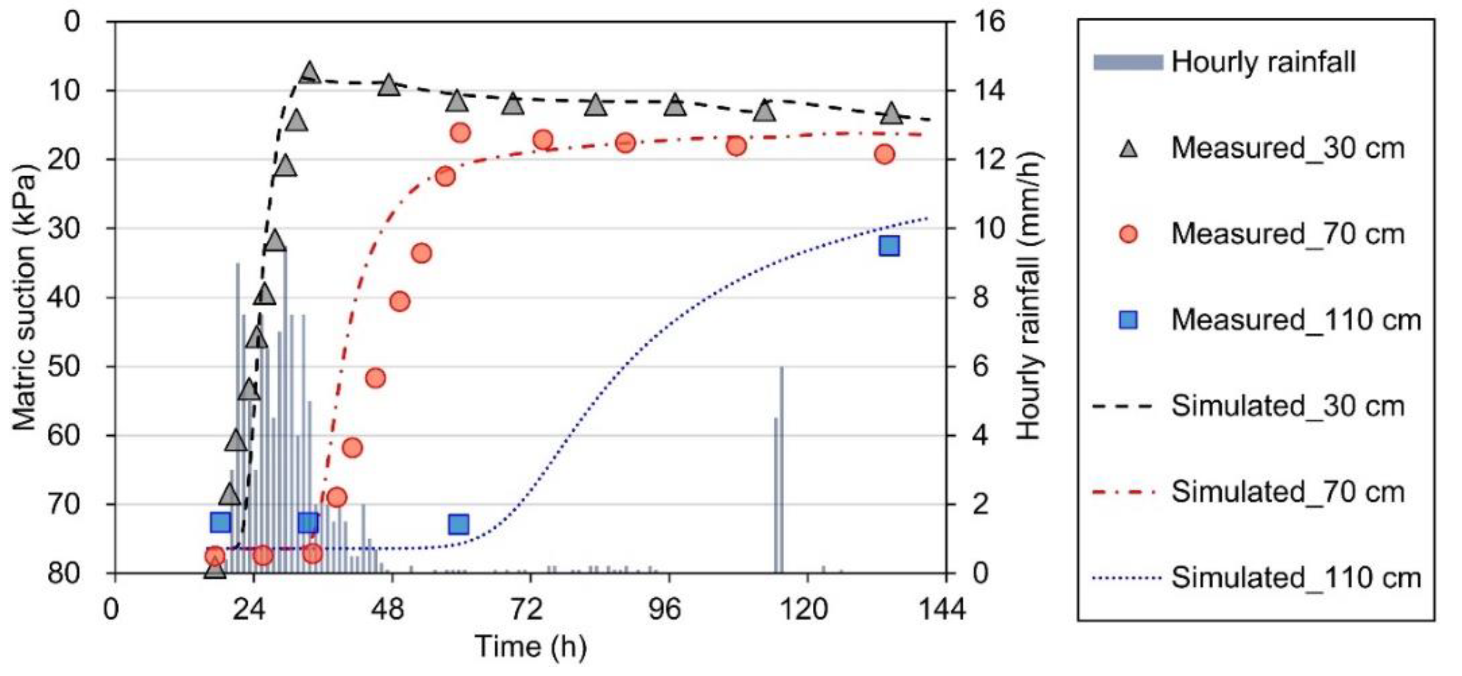
To validate the two-phase flow model utilized for infiltration simulations, we compared the matric suction measured by the Seoul Metropolitan Government [41] in the study area (zone 1) from 0:00 on 29 June 2012 to 20:00 5 July 2012 and the suction simulated from the two-phase flow model (Figure 6). We modeled an infinite slope with a depth of 2 m and an angle of 25°, applying the engineering soil properties of zone 1 summarized in Table 1. Water flux was set as equal to the hourly rainfall shown in Figure 6. Other boundary conditions were set identical to those described in the section “slope geometry and boundary/initial conditions”. Considering the initial matric suctions measured at depths of 30, 70, and 110 cm (as shown in Figure 6), we set the initial slope conditions to be hydrostatic, with an initial P w of −76 kPa (a constant value by depth). It can be observed from Figure 6 that the simulated matric suction at depths of 30, 70, and 110 cm were in good agreement with the field measurements. Therefore, we concluded that the two-phase flow model could be appropriately used to simulate rainfall infiltration in the study area.

3.2. Infiltration Analysis

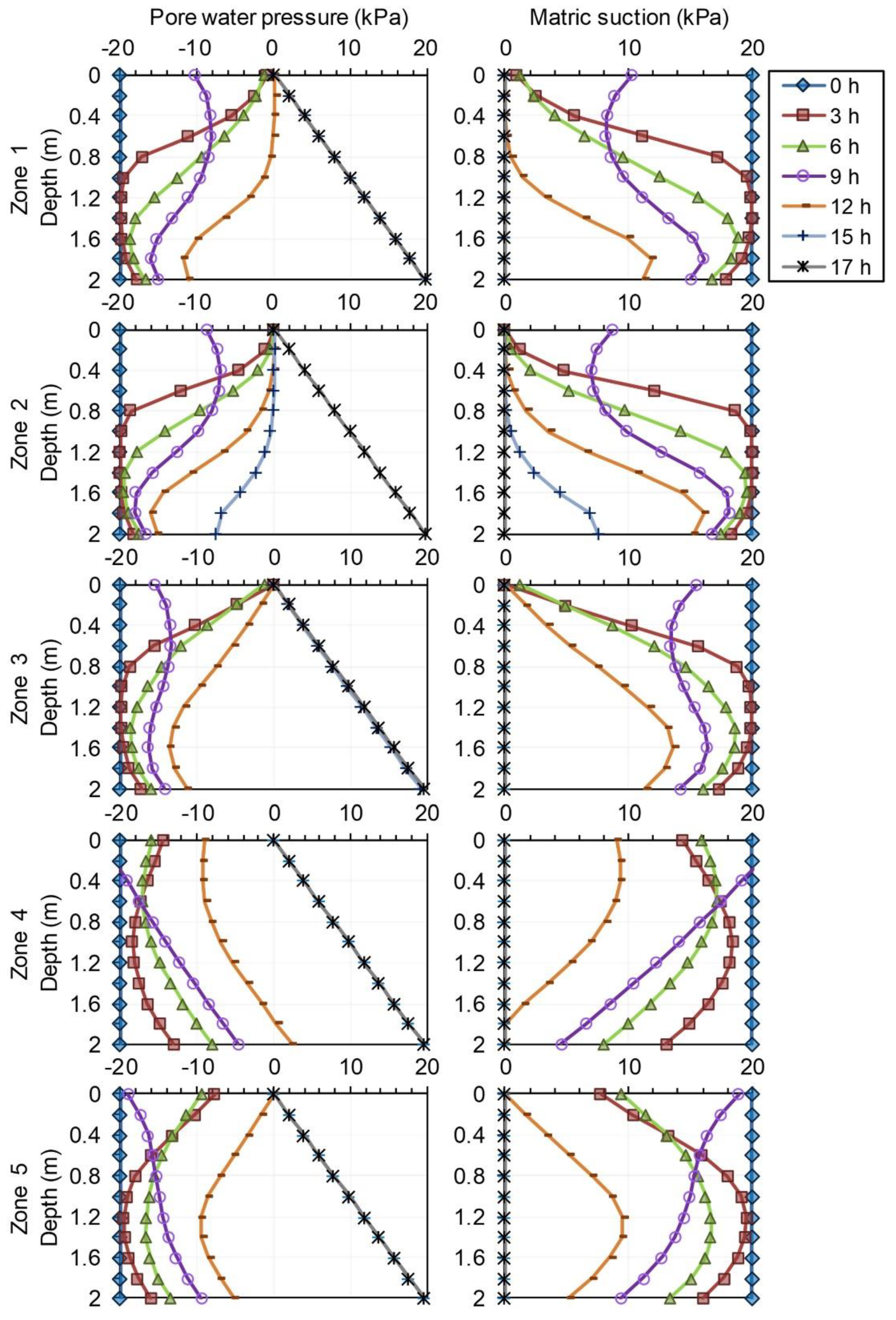
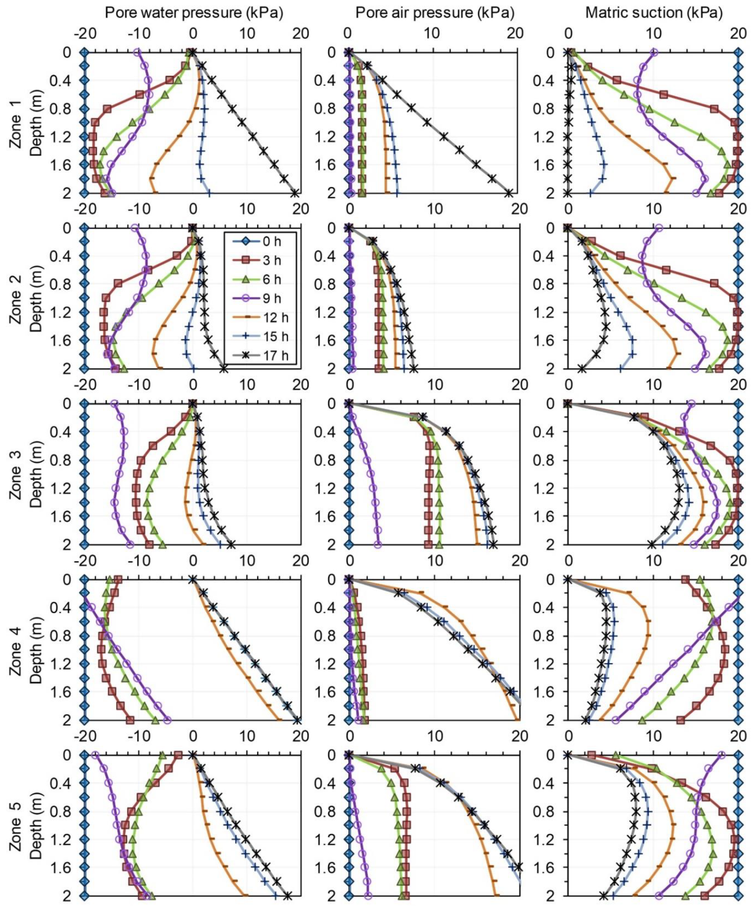
We conducted infiltration analyses for 17 h (from 16:00 on July 26 to 9:00 on July 27), applying the single-phase flow and two-phase flow models to 2D infinite slopes. The representative material properties of the soil at the five zones (Figure 3b) are summarized in Table 1. Figure 7 presents an example of variations in Pw and matric suction with time at the five zones when the single-phase flow model was applied to the slope of 30°, which is approximately equal to the mean slope angle of the slope failure sites in the study area (i.e., 31.2°). The variations in Pw, Pa, and matric suction from the two-phase flow model are shown in Figure 8. In the early stages (less than 9 h), variations in Pw in the single-phase flow and two-phase flow models are similar at zones 1 and 4; ponding effects are negligible because of a high infiltration capacity with relatively high saturated hydraulic conductivities (see Table 1). However, at zones 2, 3, and 5, the ponding caused by a rainfall intensity higher than the infiltration capacity resulted in an increase in Pa under the two-phase flow model. The increases in Pa caused Pw to increase even at certain depths under the slope where the rainfall had not reached. Therefore, increases in Pw in the two-phase flow model became higher than those in the single-phase flow model. The Pw in both the models decreased at 9 h from the start owing to the negligible rainfall between 7 and 9 h (see Figure 2). After 12 h, the infiltration rates increased sharply in the single-phase flow model during heavy rainfall whereas those from the two-phase flow model increased relatively gradually during this period. This is because air pressure interrupted the water flow into the void spaces and was accompanied by ponding ([20,35,56]). This shows clearly that air pressure impacts the infiltration rate particularly in the low permeable soils where ponding effects occur frequently.
In the single-phase flow model, the matric suction sequentially dissipated from the surface without the inclusion of Pa (see Figure 7). Meanwhile, in the two-phase flow model, the matric suction was marginal at shallow depths. However, it did not dissipate owing to Pa being higher than Pw (see Figure 8).
Because the relative permeabilities at the north side were too marginal at matric suction below 20 kPa (Figure 4b), increases in Pw at the north side (zones 1 and 2) were slower than those at the south side (zones 3, 4, and 5) in both the models. An exception was zone 3, where the saturated hydraulic conductivity was the lowest (1.80 × 10⁻⁶ m/s). The infiltration rate was the highest at zone 4 owing to the largest relative permeability and saturated hydraulic conductivity (9.7 × 10⁻⁶ m/s). The ground here was almost completely saturated after 15 h (7:00 on 27 July, 2 h prior to the landslide events). The infiltration rate was the lowest at zone 2 owing to the marginal relative permeability and saturated hydraulic conductivity.
At the south side, Pw increased toward the surface and larger depths, whereas at the north side, it increased first at shallow depths and subsequently at larger depths as the wetting bands progressed gradually into the depths because of the marginal relative permeability. In the two-phase flow model, positive Pw occurred at shallow depths because of ponding effects and heavy rainfall (after 12 h). However, the matric suction was not dissipated completely in the shallow areas because here, Pa is higher than Pw (i.e., not fully saturated).

3.3. Slope Stability Assessment

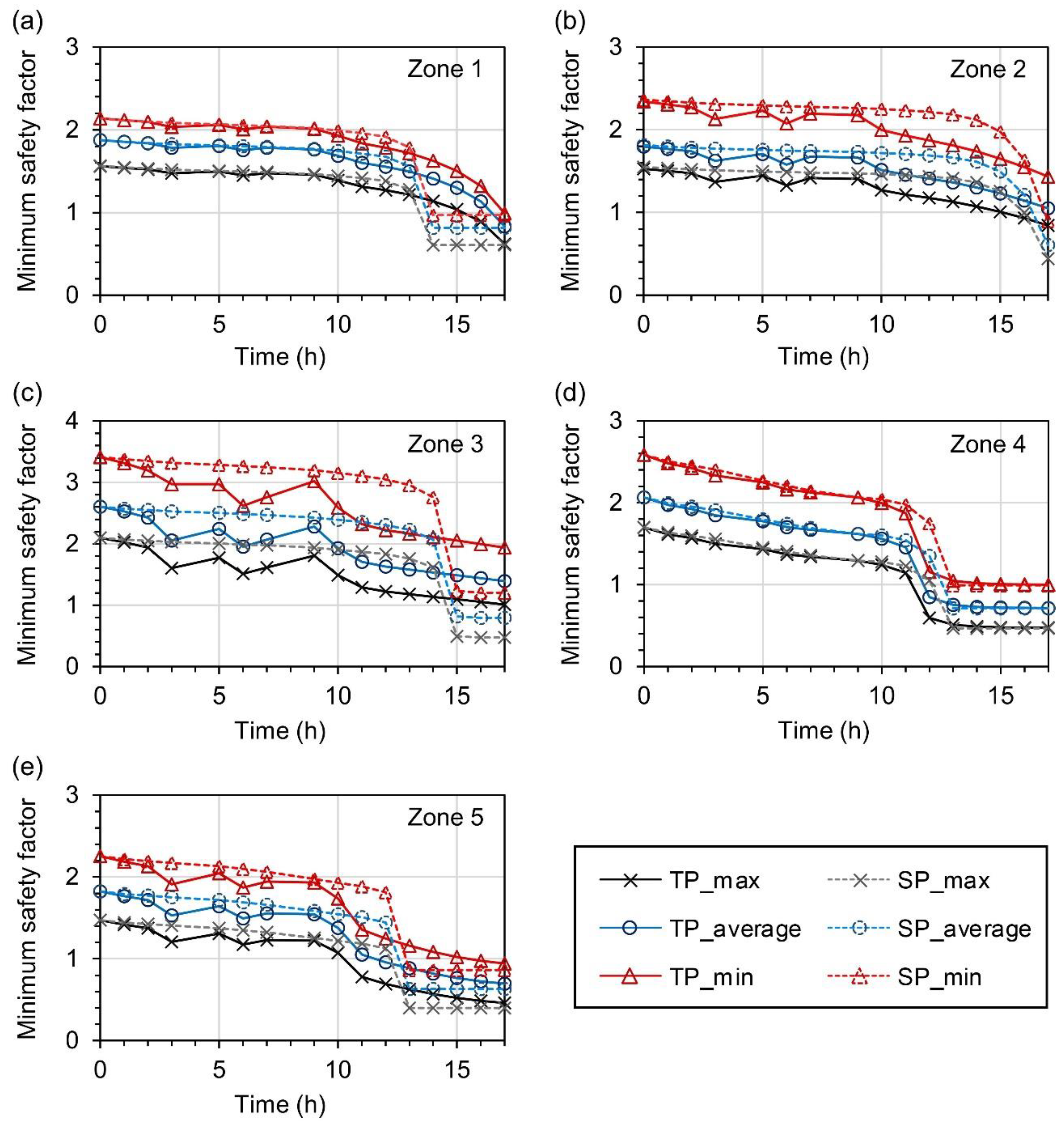
The safety factor is dependent on shear strength parameters (i.e., internal friction angle and cohesion) and variations in Pw and Pa. Figure 9 shows the variations in the minimum safety factors on infinite slopes whose angles are the maximum, average, and minimum of the actual slope failure sites at each zone. The initial safety factors at zone 3 are larger than those at the other zones, with values higher than 3 (Figure 9c) owing to the large internal friction angle (37.6°) and high cohesion (7.7 kPa). Initial safety factors on slopes with the average angles at zones 1, 2, and 5, where the internal friction angles and cohesions are marginal (see Table 1), are smaller than two (Figure 9a,b,e). At the north side (zones 1 and 2), the safety factors decreased gradually owing to gradual infiltration rates and reduced abruptly after 13 h. Meanwhile, at the south side (zones 3, 4, and 5), the safety factors reduced gradually from the initial values and decreased to below one more rapidly than those at the north side. This is owing to the rapid infiltration (with an exception of zone 3 because of the smallest saturated hydraulic conductivity (1.8 × 10⁻⁶ m/s)). Therefore, hydrological properties (i.e., saturated hydraulic conductivity and relative permeability) strongly affect variations in the safety factor, thereby influencing infiltration rates.
The safety factors from both the single- and two-phase flow models were similar during the early stages. However, the decrease in the safety factor in the two-phase flow model became higher than that in the single-phase flow model during the middle stages owing to the effects of ponding. Whereas the decrease in the effective stress resulted solely from the increase in Pw in the single-phase flow model, the increases in both Pw and Pa in the two-phase flow model resulted in a higher decrease in the safety factor. This is because the shear strength decreased as Pw and Pa increased (referring to Equation (13)). However, the safety factor in the single-phase flow model became lower than that in the two-phase flow model during the final stage. This is because the slopes in the single-phase flow model became saturated more rapidly than those in the two-phase flow model (as shown in Figure 7 and Figure 8). These observations are comparable with the observations of Cho [11].
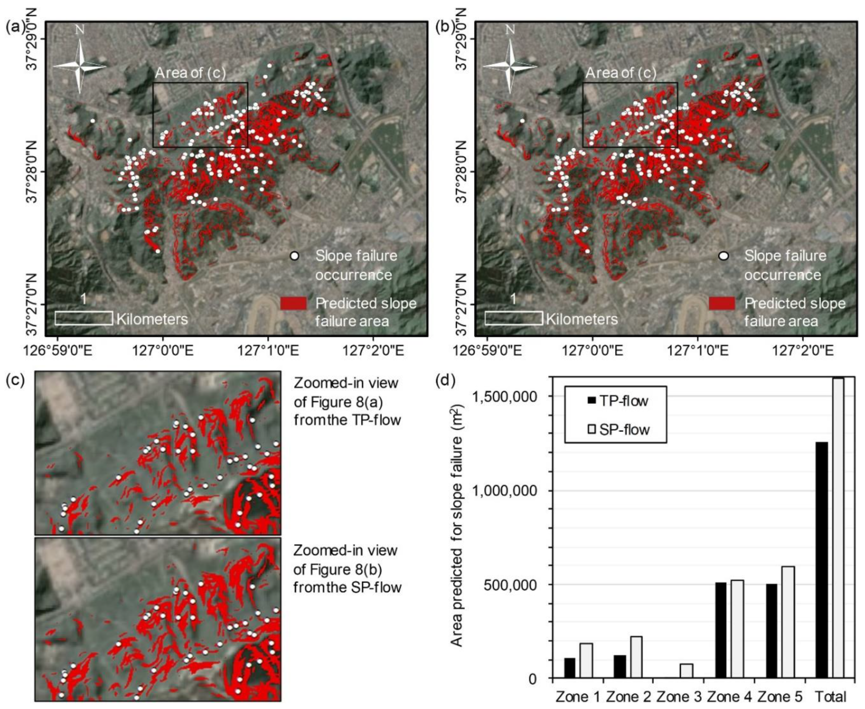
We generated landslide susceptibility maps for Umyeon Mountain based on topographic maps (i.e., DEM and slope map) with a cell size of 10 m, the geotechnical properties summarized in Table 1, and the distributions of Pw and Pa obtained from infiltration analyses by applying the single-phase flow and two-phase flow models in FLAC (Figure 10a,b). The distribution patterns for the areas of predicted slope failure are similar because the same topographic maps and geotechnical properties were applied to generate both maps. However, applying different models resulted in differences in the total area predicted for slope failure, as shown in Figure 10c,d. On the north side (zones 1 and 2), the total area of potential slope failure in the two-phase flow model (234,600 m2) is smaller than that in the single-phase flow model (405,525 m2). This is because the rainfall infiltration at the north side is slower in the two-phase flow model than it is in the single-phase flow model.
At zones 4 and 5, the slope failure areas predicted from the two- and single-phase flow models (1,018,925 and 1,189,575 m2, respectively) are similarly distributed because the ground approached saturated conditions owing to rapid infiltration with large relative permeabilities. However, under the application of the two-phase flow model, the potential slope failure areas are markedly marginal in Zone 3 because of the considerable matric suction there (as shown in Figure 8). This is comparable with the fact that there was no actual slope failure in zone 3 with a large representative internal friction angle of 37.6°.
We then applied the modified success rate (MSR) to evaluate the quantitative prediction performance for the slope failure areas. In total, 161 actual slope failures occurred in the study area, and the total number of slope failures that were successfully predicted by the two- and single-phase flow models was 148 and 150, respectively. Therefore, the performance values produced by the former success rate (SR) for the three models are 0.92 (= 148/161) and 0.93 (= 150/161), respectively. The MSRs for both models are 0.86 and 0.84, respectively, and the stable cell coverage over the total watershed area is 80.1 and 74.7, respectively. Huang and Kao [55] reported that the best simulation could be achieved by MSR, where the stable cell coverage in a total watershed area ranges from 80% to 90%. Landslide over-prediction is likely to occur when the stable cell coverage is less than 80%, and under-prediction is likely when it is larger than 90%.
The largest MSR was derived from the two-phase flow model, where an adequate range of stable cell coverage was used for the best simulation (i.e., 80%–90%). The largest SR was derived from the single-phase flow model. However, the MSR-derived value was the second largest in this case, owing to the lesser stable cell coverage that probably causes an over-prediction of landslides.
Table 3 summarizes the results of the performance evaluation of the two- and single-phase flow models utilizing the confusion matrix. True positive (TP), true negative (TN), false positive (FP), and false negative (FN) for the two-phase flow model are respectively 0.23%, 80.11%, 19.64%, and 0.02%, and those for the single-phase flow model are 0.24%, 74.69%, 25.05%, and 0.02%, respectively. Efficiency, positive predictive power, sensitivity, and specificity were computed from the confusion matrix to quantitatively evaluate the estimation performance. The efficiency means the proportion of correctly predicted class and is most frequently used in the literature [54]. The efficiency of the two-phase flow model (80.19%) was greater than that of the single-phase flow model (74.79%). The positive predictive power means the proportion of TP in a total of positive predicted class. Low values of TP resulted from both the two- and single-phase flow models (0.23% and 0.24%, respectively). This is because a number of actual slope failure sites (161 cells) were quite small compared to the mountainous area considered in this study (63,157 cells). Even if all the actual slope failure sites are correctly predicted, the maximum value of TP is 0.25% (161/63,157). Therefore, regardless of the method of analysis, the value of the positive predictive power is consequently low. The positive predictive power of the two-phase flow model (1.17%) was slightly larger than that of the single-phase flow model (0.93%) due to the large FP, resulting in an over-prediction of landslides. Only for the sensitivity that is the same as the SR used to compute the MSR, the result from the single-phase flow model (93.17%) was better than that from the two-phase flow model (91.93%). As for the specificity, which is the proportion of negative observations accurately predicted, the two-phase flow model resulted in a greater value (80.16%) than the single-phase flow model (74.74%). Given the performance values produced by the MSR and confusion matrix, the two-phase flow model exhibits good agreement with the actual landslide events at Umyeon Mountain.

4. Conclusions

Although air flow changes the infiltration rate of rainfall and variations in the safety factor of unsaturated soils, it has rarely been considered. We applied the two-phase (water and air) flow model to infiltration and slope stability analysis and assessed the model applicability for the Umyeon Mountain landslides that occurred in 2011. We used the available historical rainfall data, topographic maps, and geotechnical/hydrological properties to construct the model. Location information of the actual slope failures, the MSR, and the confusion matrix were used to evaluate the model performance. The following are interpretations of the results of the infiltration and slope stability analyses:
  • Considering that air flow changes the rate of increase in Pw on slopes with a low infiltration capacity when ponding occurs during heavy rainfall, and that the saturated hydraulic conductivity is relatively marginal in the mountainous areas of Korea (i.e., less than 2.78 × 10⁻⁵ m/s according to the National Disaster Management Institute [57]), it is necessary to apply the two-phase flow model to accurately interpret rainfall infiltration.
  • The initial safety factor prior to rainfall depends on the shear strength parameters (i.e., internal friction angle and cohesion); however, variations in the safety factor are strongly dependent on an increase in the Pw rate. Slopes in the single-phase flow model rapidly become saturated during heavy rainfall because of the high rainfall infiltration rates without the interruption of air. Thus, safety factors decrease rapidly compared to those in the two-phase flow model.
  • Landslide susceptibility maps change depending on an increase in Pw, which depends on relative permeability. It is also sensitive to the model type. The MSR and confusion matrix yield the highest performance for the two-phase flow model with an appropriate range of stable cell coverage for the best simulation. Thus, it is concluded that infiltration and slope stability analyses using the two-phase flow model have good applicability in evaluating landslide events in Umyeon Mountain. However, it is necessary to additionally evaluate the applicability of this model for other landslide cases.
  • We performed infiltration and slope stability analyses focusing on the geotechnical characteristics of unsaturated soils in the upper layer. Besides, we excluded geological characteristics given that most of the slope failure in the study area occurred at the colluvium layer with shallow depths up to 2 m. The two-phase flow model can be usefully applied to the region where shallow slope failure occurs primarily. However, further study is required to examine the effects of the geological structure for improving the applicability of the two-phase flow model to the region where deep slope failure occurs primarily, which is affected not only by geotechnical characteristics but also by geological structure.
  • The performance of slope stability assessments at a regional scale is greatly affected by the uncertainty and variability of geotechnical and hydrological input parameters when physically based models are applied. Geotechnical and hydrological properties have probabilistically or statistically been characterized based on types of soil and lithology to properly consider the uncertainty and variability of them [58,59], whereas we used representative constant soil properties at each of the five zones as averaged from field measurements. The applicability of the two-phase flow model to a regional scale can be improved by further study applying the probabilistic approach for characterizing the uncertainty and variability of geotechnical and hydrological input parameters.

Author Contributions

All authors significantly contributed to the research. S.K. acquired data and wrote an original draft. S.-E.C. contributed to interpreting results. B.K. reviewed and edited the paper. G.-H.G. designed this research. All authors have read and agreed to the published version of the manuscript.

Funding

This research was funded by Kumoh National Institute of Technology, grant number 2019-104-166.

Acknowledgments

This work was supported by Kumoh National Institute of Technology (2019-104-166).

Conflicts of Interest

The authors declare no conflict of interest.

References

  1. Chen, H.-E.; Tsai, T.-L.; Yang, J.-C. Threshold of Slope Instability Induced by Rainfall and Lateral Flow. Water 2017, 9, 722. [Google Scholar] [CrossRef] [Green Version]
  2. Haque, U.; da Silva, P.F.; Devoli, G.; Pilz, J.; Zhao, B.; Khaloua, A.; Wilopo, W.; Andersen, P.; Lu, P.; Lee, J.; et al. The human cost of global warming: Deadly landslides and their triggers (1995–2014). Sci. Total Environ. 2019, 682, 673–684. [Google Scholar] [CrossRef] [PubMed]
  3. Cho, S.E. Study on the characteristics of infinite slope failures by probabilistic seepage analysis. J. Korean Geotech. Soc. 2014, 30, 5–18. [Google Scholar] [CrossRef] [Green Version]
  4. McGuire, L.A.; Rengers, F.K.; Kean, J.W.; Coe, J.A.; Mirus, B.B.; Baum, R.L.; Godt, J.W. Elucidating the role of vegetation in the initiation of rainfall-induced shallow landslides: Insights from an extreme rainfall event in the Colorado Front Range. Geophys. Res. Lett. 2016, 43, 9084–9092. [Google Scholar] [CrossRef] [Green Version]
  5. Johnson, J.M.; Loáiciga, H.A. Coupled Infiltration and Kinematic-Wave Runoff Simulation in Slopes: Implications for Slope Stability. Water 2017, 9, 327. [Google Scholar] [CrossRef] [Green Version]
  6. Ehlers, W.; Avci, O.; Markert, B. Computation of Slope Movements Initiated by Rain–Induced Shear Bands in Small–Scale Tests and In Situ. Vadose Zone J. 2011, 10, 512–525. [Google Scholar] [CrossRef]
  7. Germer, K.; Braun, J. Effects of Saturation on Slope Stability: Laboratory Experiments Utilizing External Load. Vadose Zone J. 2011, 10, 477–486. [Google Scholar] [CrossRef]
  8. Wienhöfer, J.; Lindenmaier, F.; Zehe, E. Challenges in Understanding the Hydrologic Controls on the Mobility of Slow-Moving Landslides. Vadose Zone J. 2011, 10, 496–511. [Google Scholar] [CrossRef]
  9. Cho, S.E.; Lee, S.R. Instability of unsaturated soil slopes due to infiltration. Comput. Geotech. 2001, 28, 185–208. [Google Scholar] [CrossRef]
  10. Ng, C.W.W.; Shi, Q. A numerical investigation of the stability of unsaturated soil slopes subjected to transient seepage. Comput. Geotech. 1998, 22, 1–28. [Google Scholar] [CrossRef]
  11. Cho, S.E. Stability analysis of unsaturated soil slopes considering water–air flow caused by rainfall infiltration. Eng. Geol. 2016, 211, 184–197. [Google Scholar] [CrossRef]
  12. Yeh, H.F.; Lee, C.H.; Lee, C.C. A rainfall–infiltration model for unsaturated soil slope stability. Sustain. Environ. Res. 2008, 18, 271–278. [Google Scholar]
  13. Thomas, M.A.; Mirus, B.B.; Collins, B.D. Identifying Physics-Based Thresholds for Rainfall-Induced Landsliding. Geophys. Res. Lett. 2018, 45, 9651–9661. [Google Scholar] [CrossRef]
  14. Richards, L.A. Capillary conduction of liquids through porous mediums. Physics 1931, 1, 318–333. [Google Scholar] [CrossRef]
  15. Jeong, S.; Lee, K.; Kim, J.; Kim, Y. Analysis of Rainfall-Induced Landslide on Unsaturated Soil Slopes. Sustainability 2017, 9, 1280. [Google Scholar] [CrossRef] [Green Version]
  16. Tran, T.V.; Lee, G.; An, H.; Kim, M. Comparing the performance of TRIGRS and TiVaSS in spatial and temporal prediction of rainfall-induced shallow landslides. Environ. Earth Sci. 2017, 76, 315. [Google Scholar] [CrossRef]
  17. Borja, R.I.; White, J.A. Continuum deformation and stability analyses of a steep hillside slope under rainfall infiltration. Acta Geotech. 2010, 5, 1–14. [Google Scholar] [CrossRef]
  18. Borja, R.I.; White, J.A.; Liu, X.; Wu, W. Factor of safety in a partially saturated slope inferred from hydro–mechanical continuum modeling. Int. J. Numer. Anal. Methods Geomech. 2012, 36, 236–248. [Google Scholar] [CrossRef] [Green Version]
  19. Hu, R.; Hong, J.-M.; Chen, Y.-F.; Zhou, C.-B. Hydraulic hysteresis effects on the coupled flow–deformation processes in unsaturated soils: Numerical formulation and slope stability analysis. Appl. Math. Model. 2018, 54, 221–245. [Google Scholar] [CrossRef]
  20. Liu, G.; Tong, F.-G.; Zhao, Y.-T.; Tian, B. A force transfer mechanism for triggering landslides during rainfall infiltration. J. Mt. Sci. 2018, 15, 2480–2491. [Google Scholar] [CrossRef]
  21. Sun, D.M.; Zang, Y.G.; Semprich, S. Effects of airflow induced by rainfall infiltration on unsaturated soil slope stability. Transp. Porous Media 2015, 107, 821–841. [Google Scholar] [CrossRef]
  22. Wu, L.Z.; Zhang, L.M.; Zhou, Y.; Li, B.E. Analysis of multi-phase coupled seepage and stability in anisotropic slopes under rainfall condition. Environ. Earth Sci. 2017, 76, 469. [Google Scholar] [CrossRef]
  23. Zhang, X.Y.; Zhu, Y.M.; Fang, C.H. The role for air flow in soil slope stability analysis. J. Hydrodyn. 2009, 21, 640–646. [Google Scholar] [CrossRef]
  24. Chen, P.; Mirus, B.; Lu, N.; Godt, J.W. Effect of Hydraulic Hysteresis on Stability of Infinite Slopes under Steady Infiltration. J. Geotech. Geoenviron. Eng. 2017, 143, 04017041. [Google Scholar] [CrossRef] [Green Version]
  25. Ebel, B.A.; Loague, K.; Borja, R.I. The impacts of hysteresis on variably saturated hydrologic response and slope failure. Environ. Earth Sci. 2010, 61, 1215–1225. [Google Scholar] [CrossRef]
  26. Simoni, S.; Zanotti, F.; Bertoldi, G.; Rigon, R. Modelling the probability of occurrence of shallow landslides and channelized debris flows using GEOtop-FS. Hydrol. Process. 2008, 22, 532–545. [Google Scholar] [CrossRef]
  27. Rigon, R.; Bertoldi, G.; Over, T.M. GEOtop: A Distributed Hydrological Model with Coupled Water and Energy Budgets. J. Hydrometeorol. 2006, 7, 371–388. [Google Scholar] [CrossRef]
  28. Chen, L.-K.; Chang, C.-H.; Liu, C.-H.; Ho, J.-Y. Application of a Three-Dimensional Deterministic Model to Assess Potential Landslides, a Case Study: Antong Hot Spring Area in Hualien, Taiwan. Water 2020, 12, 480. [Google Scholar] [CrossRef] [Green Version]
  29. Reid, M.E.; Christian, S.B.; Brien, D.L.; Henderson, S.T. Scoops3D—Software to Analyze Three-Dimensional Slope Stability Throughout a Digital Landscape (Version 1.0); U.S. Geological Survey: Reston, VA, USA, 2015.
  30. Park, D.W.; Lee, S.R.; Vasu, N.N.; Kang, S.H.; Park, J.Y. Coupled model for simulation of landslides and debris flows at local scale. Nat. Hazards 2016, 81, 1653–1682. [Google Scholar] [CrossRef]
  31. Tran, T.V.; Alvioli, M.; Lee, G.; An, H.U. Three-dimensional, time-dependent modeling of rainfall-induced landslides over a digital landscape: A case study. Landslides 2018, 15, 1071–1084. [Google Scholar] [CrossRef]
  32. GEO-SLOPE International. User’s Manual: SEEP/W and SLOPE/W; Geo-Slope International Ltd.: Calgary, AB, Canada, 2012. [Google Scholar]
  33. Baum, R.L.; Savage, W.Z.; Godt, J.W. TRIGRS—A Fortran Program for Transient Rainfall Infiltration and Grid-based Regional Slope-stability Analysis, Version 2.0; US Geological Survey Open-File Report 2008-1159; US Geological Survey: Reston, VA, USA, 2008; p. 75.
  34. An, H.; Viet, T.T.; Lee, G.; Kim, Y.; Kim, M.; Noh, S.; Noh, J. Development of time-variant landslide-prediction software considering three-dimensional subsurface unsaturated flow. Environ. Model. Softw. 2016, 85, 172–183. [Google Scholar] [CrossRef]
  35. Dong, H.; Huang, R.; Gao, Q.-F. Rainfall infiltration performance and its relation to mesoscopic structural properties of a gravelly soil slope. Eng. Geol. 2017, 230, 1–10. [Google Scholar] [CrossRef]
  36. Touma, J.; Vauclin, M. Experimental and Numerical Analysis of Two Phase Infiltration in a Partially Saturated Soil. Transp. Porous Media 1986, 1, 27–55. [Google Scholar] [CrossRef]
  37. National Geographic Information Institute of Korea. Available online: http://map.ngii.go.kr/mn/mainPage.do (accessed on 15 August 2019).
  38. Kang, S.; Lee, S.-R. Debris flow susceptibility assessment based on an empirical approach in the central region of South Korea. Geomorphology 2018, 308, 1–12. [Google Scholar] [CrossRef]
  39. Kang, S.; Lee, S.-R.; Vasu, N.N.; Park, J.-Y.; Lee, D.-H. Development of an initiation criterion for debris flows based on local topographic properties and applicability assessment at a regional scale. Eng. Geol. 2017, 230, 64–76. [Google Scholar] [CrossRef]
  40. Korea Meteorological Administration. Available online: http://www.weather.go.kr/weather/observation/aws_table_popup.jsp (accessed on 7 March 2019).
  41. Seoul Metropolitan Government. Causes Survey and Restoration Work of Mt. Umyeon Landslides; Seoul Metropolitan Government: Seoul, Korea, 2014; p. 435.
  42. Korean Geotechnical Society. Research Contract Report: Addition and Complement Causes Survey of Mt. Umyeon Landslides; Society, K.G., Ed.; Korean Geotechnical Society: Seoul, Korea, 2011; p. 268. [Google Scholar]
  43. van Genuchten, M.T. A closed-form equation for predicting the hydraulic conductivity of unsaturated soils. Soil Sci. Soc. Am. J. 1980, 44, 892–898. [Google Scholar] [CrossRef] [Green Version]
  44. Fredlund, D.G.; Rahardjo, H. Soil Mechanics for Unsaturated Soils; John Wiley & Sons, Inc.: Hoboken, NJ, USA, 1993. [Google Scholar]
  45. Korea Institue of Geoscience and Mineral Resources. Available online: https://mgeo.kigam.re.kr/ (accessed on 3 March 2020).
  46. Itasca. User’s Manual: Fluid–Mechanical Interaction, FLAC 7.0; Itasca Consulting Group, Inc.: Minneapolis, MN, USA, 2011. [Google Scholar]
  47. Mualem, Y. A new model for predicting the hydraulic conductivity of unsaturated porous media. Water Resour. Res. 1976, 12, 513–522. [Google Scholar] [CrossRef] [Green Version]
  48. Lenhard, R.J.; Parker, J.C. A model for hysteretic constitutive relations governing multiphase flow: 2. Permeability-saturation relations. Water Resour. Res. 1987, 23, 2197–2206. [Google Scholar] [CrossRef]
  49. Bishop, A.W. The principle of effective stress. Teknisk Ukeblad 1959, 106, 859–863. [Google Scholar]
  50. Chateau, X.; Dormieux, L. Micromechanics of Unsaturated Porous Media. In IUTAM Symposium on Theoretical and Numerical Methods in Continuum Mechanics of Porous Materials; Solid Mechanics and Its Applications, Vol 87; Ehlers, W., Ed.; Springer: Berlin/Heidelberg, Germany, 2001; pp. 125–130. [Google Scholar]
  51. Chateau, X.; Dormieux, L. Micromechanics of saturated and unsaturated porous media. Int. J. Numer. Anal. Methods Geomech. 2002, 26, 831–844. [Google Scholar] [CrossRef]
  52. Zhang, L.; Wu, F.; Zheng, Y.; Chen, L.; Zhang, J.; Li, X. Probabilistic calibration of a coupled hydro-mechanical slope stability model with integration of multiple observations. Georisk Assess. Manag. Risk Eng. Syst. Geohazards 2018, 12, 169–182. [Google Scholar] [CrossRef]
  53. Kim, J.; Jeong, S.; Park, S.; Sharma, J. Influence of rainfall-induced wetting on the stability of slopes in weathered soils. Eng. Geol. 2004, 75, 251–262. [Google Scholar] [CrossRef]
  54. Beguería, S. Validation and Evaluation of Predictive Models in Hazard Assessment and Risk Management. Nat. Hazards 2006, 37, 315–329. [Google Scholar] [CrossRef] [Green Version]
  55. Huang, J.C.; Kao, S.J. Optimal estimator for assessing landslide model performance. Hydrol. Earth Syst. Sci. 2006, 10, 957–965. [Google Scholar] [CrossRef] [Green Version]
  56. Hu, R.; Chen, Y.; Zhou, C. Modeling of coupled deformation, water flow and gas transport in soil slopes subjected to rain infiltration. Sci. China Technol. Sci. 2011, 54, 2561. [Google Scholar] [CrossRef]
  57. National Disaster Management Institute. Study on the Secure Plan for the Stability of Slope Based on Ground Characteristics; Report no.: 11-1311526-000053-01; National Disaster Management Institute: Seoul, Korea, 2012; p. 138.
  58. Salciarini, D.; Fanelli, G.; Tamagnini, C. A probabilistic model for rainfall–induced shallow landslide prediction at the regional scale. Landslides 2017, 14, 1731–1746. [Google Scholar] [CrossRef]
  59. Tofani, V.; Bicocchi, G.; Rossi, G.; Segoni, S.; D’Ambrosio, M.; Casagli, N.; Catani, F. Soil characterization for shallow landslides modeling: A case study in the Northern Apennines (Central Italy). Landslides 2017, 14, 755–770. [Google Scholar] [CrossRef] [Green Version]
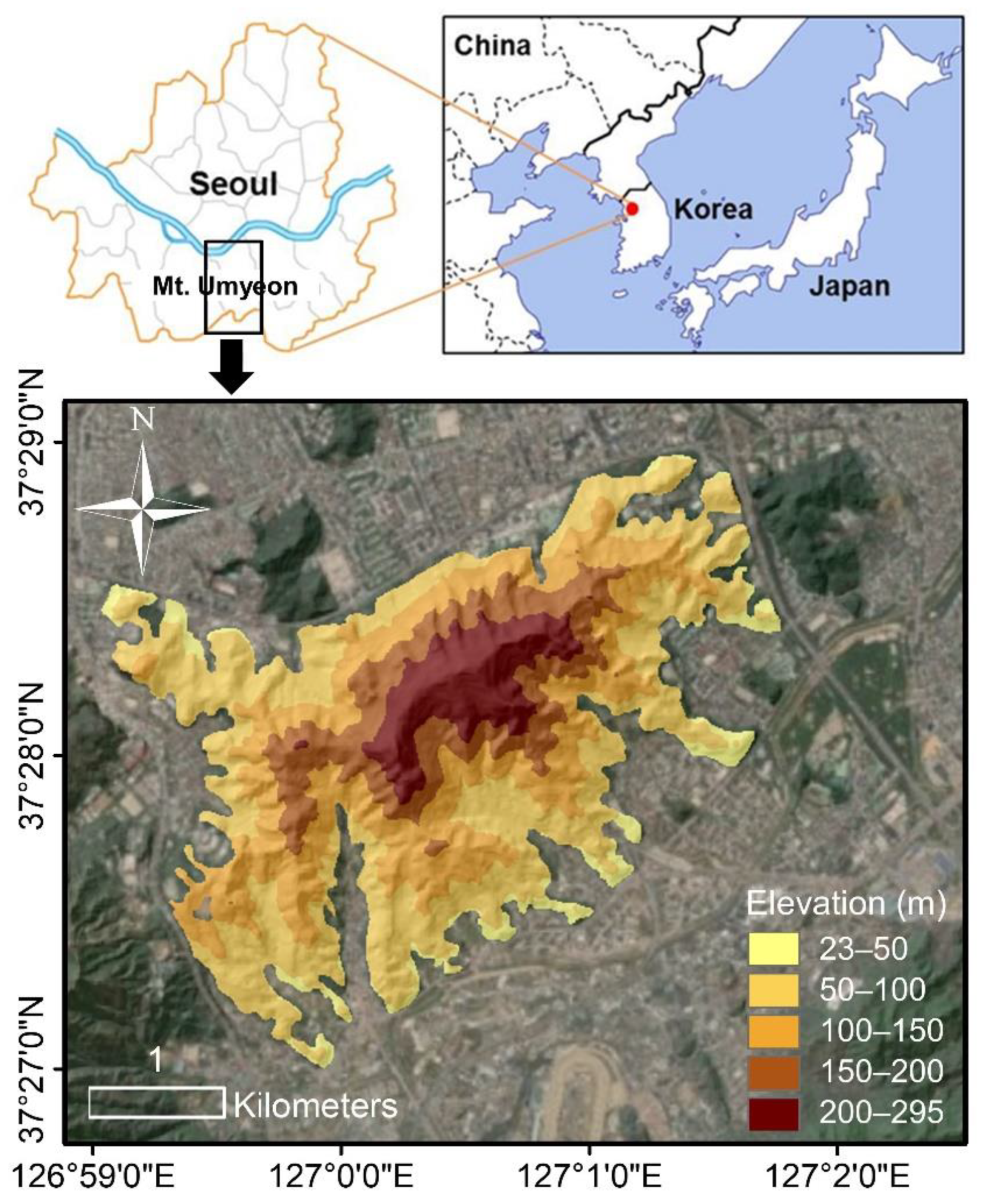
Figure 1. Location and elevation distributions of Umyeon Mountain.
Water 12 00812 g001
Figure 2. Hourly rainfall and cumulative rainfall recorded at the Namhyun station during the two days from 26 July to 27 July 2011 (obtained from KMA).
Water 12 00812 g002
Figure 3. (a) Locations where slope failure occurred in the area of Umyeon Mountain in 2011. (b) Geology map of the study area produced by the Korea Institute of Geoscience and Mineral resources [45] and locations of three sites (BL-1, BL-2, and BL-3) at which boring investigations were performed. (c) Boring logs and groundwater levels obtained at three sites shown in (b) (modified from the Seoul Metropolitan Government [41]). (d) Locations of the sites’ selected borehole for the investigation conducted by the Seoul Metropolitan Government [41] and the distribution of the five zones proposed by Park et al. [30].
Water 12 00812 g003
Figure 4. (a) van Genuchten soil-water characteristic curves (SWCCs) for the north side of Umyeon Mountain (zones 1 and 2) and its south side (zones 3, 4, and 5) (obtained from Seoul Metropolitan Government [41]). (b) Relative permeability (Kr) curves computed from the two SWCCs shown in Figure 4a. The constants of the two van Genuchten SWCCs used to compute Mualem–van Genuchten relative permeability curves [43] are presented in Table 1.
Water 12 00812 g004
Figure 5. An example of the infinite slope model and finite difference discretization for infiltration analysis with a depth of 2 m, a length of 10 m, and an angle of 31°, which is approximately equal to the mean slope angle of the slope failure sites in the study area (i.e., 31.2°). Various angles were considered based on different cells of the GIS-based slope raster. q w , I ( t ) , P a , P w , u x , and u y denote water flux, variations in rainfall intensity with time, pore water and air pressures, displacements in the horizontal and vertical directions, respectively.
Water 12 00812 g005
Figure 6. Comparison between measured and simulated matric suction for 140 h (from 0:00 on 29 June 2012 to 20:00 5 July 2012).
Water 12 00812 g006
Figure 7. Variations in pore water pressure and matric suction with time when the single-phase flow model was applied to a slope of 30°. The vertical axis of each graph represents the depth from the ground surface. The first and second columns represent the ranges of the pore water pressure and matric suction, respectively.
Water 12 00812 g007
Figure 8. Variations in pore water/air pressures and matric suction with time when the two-phase flow model was applied to a slope of 30°. The vertical axis of each graph represents the depth from the ground surface. The columns represent the ranges of the pore water pressure, pore air pressure, and matric suction from left to right.
Water 12 00812 g008
Figure 9. Variations in minimum safety factors with time when the two- and single-phase flow models were applied to slopes with maximum, average, and minimum slope angles for actual failure slopes: (a)–(e) for zones 1–5. We used the maximum, average, and minimum slope angles for the entire actual slope failure sites in the study area only for zone 3, where an actual slope failure did not occur. The maximum, average, and minimum slope angles at zones 1–5 are 38.8°, 30.7°, and 26.5°; 37.4°, 31°, and 23.3°; 40.5°, 31.2°, and 23.3°; 40.5°, 31.8°, and 24.8°; and 40.3°, 31.1°, and 24.7°, respectively.
Water 12 00812 g009
Figure 10. Locations of slope failures and landslide susceptibility maps, which present distributions of safety factors: (a,b) from the two- and single-phase flow models using FLAC. (c) Zoomed-in views of Figure 10a,b. (d) Distribution of the slope failure area at each zone predicted by the two- and single-phase flow models.
Water 12 00812 g010
Table 1. Summary of the representative soil properties [30] and soil-water characteristics [41] for each zone used in the infiltration and slope failure analyses.
Zone No. ϕ (°) c (kPa) γ t   ( kN / m 3 ) γ d   ( kN / m 3 ) ks (m/s)Van Genuchten SWCC Coefficient
1/P0a
125.39.618.1157.15 × 10−60.0510.35
228.55.817.714.93.87 × 10−60.0510.35
337.67.717141.80 × 10−60.0380.63
430.97.617.314.59.70 × 10−60.0380.63
528.26.318.2153.69 × 10−60.0380.63
ϕ : Internal friction angle; c: Cohesion; γt: Total unit weight of soil; γd: Dry unit weight of soil; ks: Saturated hydraulic conductivity; P0: Parameter based on the air-entry value; and a: van Genuchten m constant; SWCC: soil-water characteristic curve.
Table 2. Summary of the material properties of water and air used in the infiltration analysis.
ParameterValue
Viscosity ratio, μ w   /   μ a 56
Water density, ρ w 1000 kg/m3
Air density, ρ a 1.25 kg/m3
Bulk modulus of water, Kw2 × 109 Pa
Bulk modulus of air, Ka1 × 105 Pa
Table 3. Overview of the estimation performance for slope stability assessment in the study area.
Total Probability
(Total Cells: 63,157)
TP-Flow
Actual (Observed) Class
SP-Flow
Actual (Observed) Class
PositiveNegativePositiveNegative
Predicted classPositiveTrue positive 148 (0.23%)False positive 12,498 (19.79%)True positive 150 (0.24%)False positive 15,913 (25.2%)
NegativeFalse negative 13 (0.02%)True negative 50,498 (79.96%)False negative 11 (0.02%)True negative 47,083 (74.55%)
Efficiency
(= (TP + TN)/N)
80.19%74.79%
Positive predictive power
(= TP/(TP + FP))
1.17%0.93%
Sensitivity
(= TP/(TP + FN))
91.93%93.17%
Specificity
(= TN/(FP + TN))
80.16%74.74%
Note: total number of the GIS-based topography cells in the study area (= TP + FP + FN + TN).