Case Report

Innovative Feasibility Study for the Reclamation of the Cascajo Wetlands in Peru Utilizing Sustainable Technologies

by
Keiji Jindo
1,* and
Marino S. Morikawa Sakura
2
1
Agrosystems Research Group, Wageningen University and Research, 6708PB Wageningen, The Netherlands
2
TTT Grupo Morikawa, Pueblo Libre, Lima 15084, Peru
*
Author to whom correspondence should be addressed.
Water 2020, 12(4), 1097; https://doi.org/10.3390/w12041097
Submission received: 31 January 2020 / Revised: 7 April 2020 / Accepted: 9 April 2020 / Published: 12 April 2020
(This article belongs to the Section Water Use and Scarcity)

Abstract

:
Wetlands are an important feature for our society that provides versatile benefits, such as habitat for diverse wildlife, shoreline erosion protection, flood control, and mitigation of climate change through capture and storage of carbon. The aim of this work was to assess the application of nanotechnologies for the restoration of the water quality in the Cascajo Wetlands, Peru, where the water quality was deteriorated. Ceramic-based bio-filters (CBBFs) were used to reduce and buffer the contamination rates of pollutants, whereas micro-nano bubbles (MNBs) were applied to increase the dissolved oxygen and release free radicals in water. Additionally, bio-fence was implemented to prevent water intrusion from the ocean. Remote sensing data through the Normalized Difference Vegetation Index (NDVI) and the Enhanced Vegetation Index (EVI) was used to monitor the water surface condition. With treatment of CBBFs and MNBs for 13 months, we observed reduction in the chemical oxygen demand (COD), biological oxygen demand (BOD), total nitrogen (TN), and total phosphate (TP) in the water body, showing removal percentages of 98.5%, 97.5%, 98.1%, 98.5%, and 94.6%, respectively, in comparison with values before starting the implementation. The trends of NDVI and EVI over seasons are not completely aligned with the results taken from the wetlands treated with MNBs, CBBFs and bio-fence. While TN was highly correlated with the empirical value of TN based on remote sensing, no correlation was observed between COD and empirical COD. The use of eco-friendly techniques has performed efficiently to remove the pollutant.

1. Introduction

These days, there exists increasing interest in nature-based solutions (NBS) that aim to mitigate the effects of climate change and its adaptations [1]. NBS is broadly defined as “an action to protect, sustainably manage and restore natural or modified ecosystems, which is inspired by, supported by, or copied from nature” [2,3]. Furthermore, the NBS approach needs to be fitted into the criteria of: (1) societal challenge orientation; (2) ecosystem process utilization; and (3) feasible implementation [4,5,6]. Hanson et al. [7] reviewed the current NBS research and outlined trends by grouping 112 scientific peer-reviewed articles. While 52% of the scientific papers using NBS concepts are combined with other existing concepts (e.g., “ecosystem service” and “green infrastructure”), the major themes are flood mitigation, biodiversity conservation, and functional ecosystems. As the utility of wetlands covers those three objectives, the protection and conservation of natural wetlands have been frequently chosen as an excellent example in the framework of NBS [5,8,9] due to the multi-functionalities of wetlands to provide social and economic services [10], as well as to maintain the ecological balance [11,12]. Wetlands are reservoirs for biodiversity, by not only providing a vital habitat for hundreds of species of amphibians, birds, mammals, and plants, but also giving shelter to endangered, endemic, and migratory species [13]. The soil and vegetation of wetlands filter pollutants in the water passing through these areas, rendering the water from rivers, lakes, and underground aquifers cleaner [14,15]. Healthy wetlands play a versatile role in helping adapt some of these climate changes, such as (1) contributing for flood control by collecting the excess rainwater that is subsequently released progressively; and (2) acting as water reservoirs during rainy or thawing seasons, thus buffering the effects of the floods downstream [11]. Regarding connection with other water bodies, it is well known that many wetlands contribute to the recharge of underground aquifers that store 97% of unfrozen fresh water in the world [13,16]. In other cases, water from wetlands flows underground downstream to aquifers, where the water is discharged. With its sediments and nutrient retention capacity, wetlands slow down the force of water, promoting the deposition of transported sediments and nutrients (e.g., nitrogen and phosphorus) [17]. The retention of nutrients thus makes it one of the most productive ecosystems. Wetlands also act as carbon sumps that play an essential role in retaining carbon dioxide, and which reduce the effects of global warming [11,18].
However, it is reported that 50% of wetlands have been lost since the 1900s [19]. The vulnerability of wetland resources is an important issue; they are often affected by intensive anthropogenic activities in surroundings, such as improper treatment of municipal waste disposal and wastewater discharge, as well as agricultural intensification. The Cascajo Wetlands in Peru were found to be in a severe state of pollution generated by human activities and a lack of environmental protection for over two decades. Basically, three environmental drivers affected the deterioration of water quality in Cascajo: (1) high exploitation and investment in the agricultural sector around this region by using large irrigation systems in Chancay-Huaral Basin and Chancay-Lambayeque Basin [20,21,22,23] that bring high nutrient concentrations to the wetland, causing the invasion of Pistia stratiotes [24]; (2) mining and industrial sites pollute natural water resources in this region [25]; as a consequence, the degraded water quality in the Chancay Bay, which is near the Chancay Wetlands, was detected throughout 2003–2013, due to pollutants from domestic and industrial discharges [26]; and 3) organic waste deposits from livestock enclosures nearby the wetlands contributes to the eutrophication above [27,28].
It is worthwhile to highlight that climate-related effects on wetland ecosystems are a global concern [29,30,31]. In particular, the impacts on coastal wetlands at a worldwide scale, including the Peruvian coastal region, have been reported, such as the impacts of El Niño and La Niña [32], and sea-level rise [31]. In the Northern Peruvian catchment, significant increasing trends in temperature and precipitation rates were observed over 38 years (1970–2008) [33]. In this context, it should be addressed the importance of restoration of the wetlands water quality, and removal of its aquatic vegetation, given that the wetlands have an essential function for water retention, water provision, and protection against coastal erosion, as well as sea-level rise.
A wide range of different applications have been deployed for wetland cleanup, and dredging and capping are considered as classic methods. However, sufficient evidence shows the pitfalls of these methods [34]. Dredging is a costly approach and could cause remobilization of contaminants, rendering them more bioavailable to the biota and leading to human exposure, while capping with clean neutral materials (e.g., sand, clay) has the practical approach to minimize the risk in the short-run, implying that the limited adsorption capacity and porosity of these materials reduce the efficiency for a long term [35]. With an even more sophisticated approach of active capping using sorbent material such as activated carbon or biochar, potential risk still remains with the migration of contaminants through the cap via porewater pathways [36]. Aluminum sulfate application is another popular option for wetland restoration, especially for the reduction of excess phosphorous release from sediment. However, a large number of reports show the high risk of toxicity and bioavailability in the water body by conducting this application [37,38].
Nanotechnologies and beneficial microorganisms for wetland restoration are emerging approaches which undertake less disruptive implementation [39,40]. Lactobacillus plantarum is a well-known microorganism used for the treatment of wastewater [41,42]. Furthermore, the combination of different technologies enhances the efficiency of environmental remediation [43].
Remote sensing is a recognized tool to monitor the change of water body status (e.g., lagoons, wetlands, and river basins), and Landsat Thematic Mapper (TM), which is an available imaginary dataset, enables us to cross-validate the data taken from the field [19,44,45].
While many scientific reports focus on those new technologies of water remediation at a laboratory scale [41,42], little information is known about efficiency at field level [39,40]. Therefore, this work aims to examine the effectiveness of the aforementioned new technologies to enhance the water quality and cross-validate the results, regarding environmental status between field measurements and remote sensing. The applications of the ceramic-based bio-filters (CBBFs), the micro-nano bubbles (MNBs) with the microorganism Lactobacillus plantarum, and bio-fence were conducted.

2. Materials and Methods
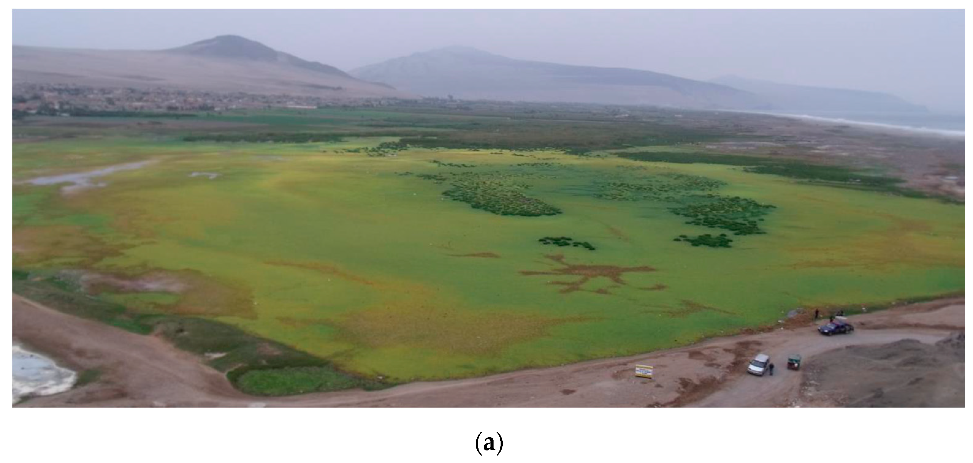
2.1. Study Site

The Cascajo Wetlands are located in Chancay, a district in the province of Huaral, department of Lima, Peru (Figure 1). The coordinates of the wetlands are as follows: (1) North 8717000 UTM; (2) East 252500 UTM. Average temperatures are between 18 and 19 °C, with maximum absolute temperatures between 25 and 28 °C and minimum temperatures between 12 and 15 °C. There is little rainfall, which averages 18 mm, with a maximum and minimum annual rainfall of 36 mm and 0 mm, respectively. They are a part of a coastal wetland system in the Pacific Corridor and represent an ecosystem that permanently and temporarily accommodates several life forms, especially migratory birds. They also provide shelter to different groups of fauna and typical flora of this ecosystem. The extension of the wetlands is approximately 0.5 km2 and is integrated into the hydrological system of the Chancay river basin, receiving a minimum influx from the Pacific Ocean. These wetlands are composed of freshwater, i.e., river water, with slight salinity close to the shoreline, which is remarkably reduced by the extension of the beach between the wetlands and the ocean, which acts as a natural salinity filter [46]. Soils are loam–sandy loam, of moderate depth, with imperfect drainage in certain areas and slow surface runoff and are susceptible to flooding. Although the deterioration of water quality in these wetlands was observed over two decades, no implementation for the restoration was undertaken before this present work.

2.2. Removal of Invasive Species from Wetlands

Pistia stratiotes, commonly known as water lettuce, is a perennial monocotyledonous aquatic plant, present either naturally or through an anthropogenic introduction, in nearly all tropical and subtropical fresh waterways. It floats on the water surface, with roots hanging below the floating leaves [47]. Since the plants were covering all of the wetlands, the removal was done manually. This activity was conducted by pushing them with bamboo sticks to the edge of each sector to be removed. Approximately over 280 tons of P. stratiotes were removed and transported to a city vivarium and compost sites.

2.3. Micro-Nano Bubbles (MNBs)

The MNB equipment was designed and assembled using the following four components: (1) MNB device (MRK MS-1); (2) water pump (BAP-30); (3) air compressor (Bonelly Advanced®); (4) electric generator (Honda Powermate 5000). More detailed information on these materials is described together with pictures in Supplementary Materials. For installation of the equipment, a quadrangular-shaped platform of 4 m × 4 m was assembled using PVC tubes, and placed 6 m away from the wetlands shore. Four steel rods of 1 m length were submerged perpendicularly and attached to every corner. At the distal points, the MRK devices were installed and connected through rubber hoses and galvanized materials (to ensure a high-pressure air inlet) to the water pump and air compressor, which were placed peripherally on the wetlands shore. The MNB system devices were installed one meter deep in the wetlands with a handle attached to the surface to allow the operative personnel to move and control them (shown in Supplementary Figure S1).

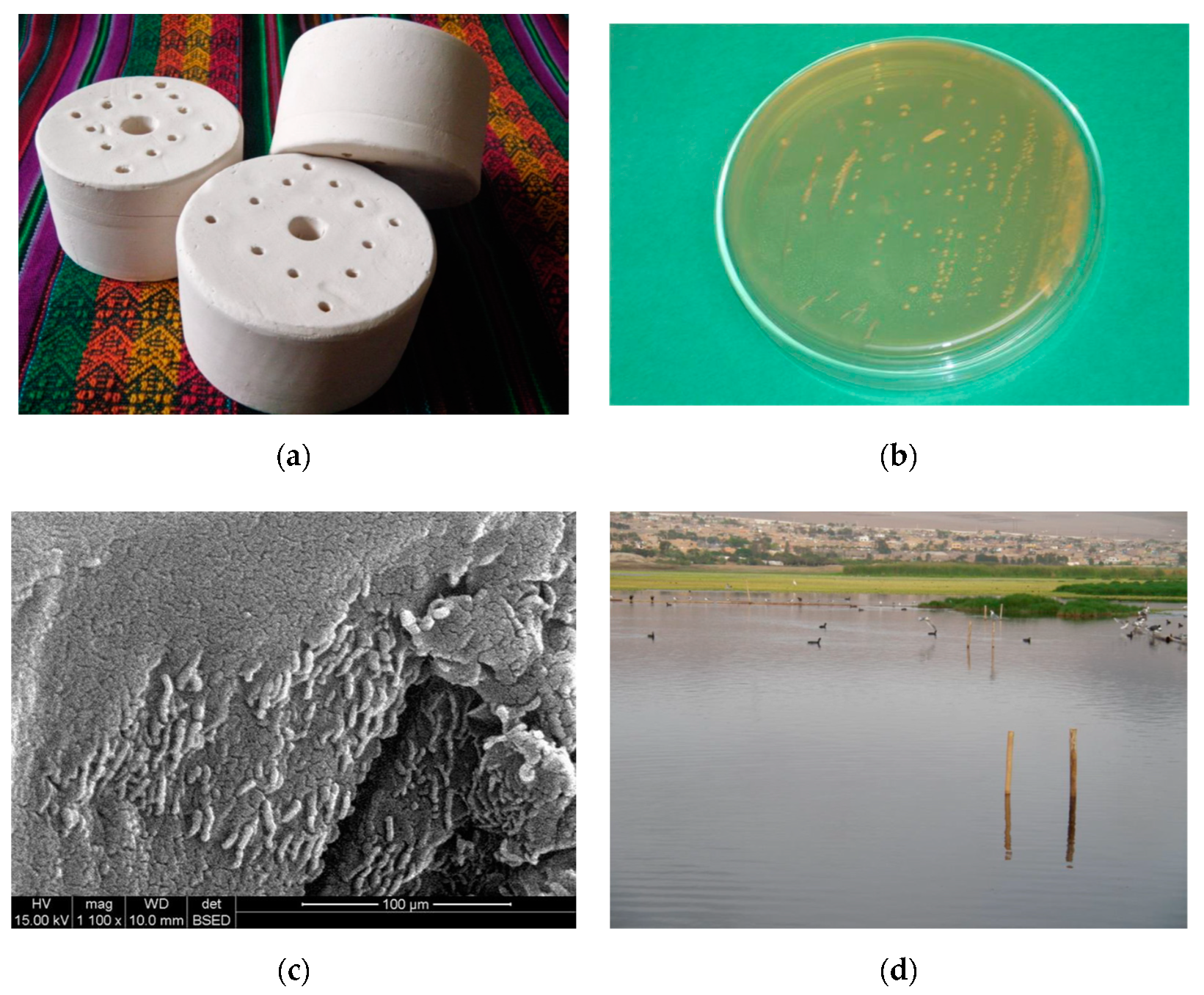
2.4. Ceramic-Based Bio-Filters (CBBFs)

The primary material used to prepare the bio-filters’ ceramic carriers was clay. It was collected and screened through a sieve number 20 (0.841 mm) for the homogenization. Then it was mixed with kaolin at a ratio of 9:1, and distilled water was added to produce a dough that was kneaded by hand to remove air bubbles to favor the process of molding. With this, mass cylindrical forms of about 10–15 cm in diameter were constructed and dried at a temperature of 80 °C for 24 h, or longer if necessary, to remove water from surface areas to avoid splitting [48]. The formed cylindrical ceramic was taken for a calcination process in a furnace at 900 °C for two hours and cooled at least for 24 h to avoid deformation of calcined materials [49]. This temperature range and duration were chosen for the optimization of the porosity of the ceramic carriers [50]. To create a bio-filter, it was necessary to effectively immobilize the bacteria and add them onto the ceramic carriers to form biofilms, which ultimately can adhere, adsorb, and decompose the contaminants [51,52]. For this purpose, we used the bacterium of Lactobacillus plantarum ATCC 8014, acquired at Japan Collection of Microorganisms (JCM), Microbe Division, RIKEN Bioresource Center in Japan. It was kept routinely in vials with full form (MRS) agar at 2–8 °C for 24 h, and then at 4 °C in 15% glycerol (vol/vol) [24]. Single colonies were cultured in plates with MRS agar at 30 °C for 48 h and later sub-cultured in MRS broth (Casein peptone 10g/L; beef extract 8 g/L; yeast extract 4 g/L; D(+) glucose 20 g/L; hydrogen potassium phosphate (KH2PO4) 2 g/L; Tween-80 1 g/L; ammonium citrate hydrogen (C6H5O7(NH4)2H) 2 g/L; sodium acetate (CH3COONa) 5 g/L; magnesium sulfate (MgSO4·7H2O) 0.2 g/L; and manganese sulfate (MnSO4·H2O) 0.04 g/L at 30 °C for 24 h [53]. The cultures in the MRS broth develop characteristic white sediment, making it easier for their qualitative identification. To create biofilms, a container of 60 cm in diameter and 130 cm in length was filled with a previously conditioned medium consisting of a mixture of molasses and water (3/7, m/w) at room temperature (around 18–21 °C). Later, Lactobacillus plantarum ATCC 8014 was added to the mixture. After 2 h, the ceramic carriers were immersed and rested for 6 days (during summer) or 3 days (during spring). This period was mandatory to immobilize Lactobacillus plantarum to form the biofilms onto the ceramic carriers’ surface, as it is shown in the scanning electron microscope (SEM) image (Figure 2). Finally, several supports and wooden baskets were arranged and placed with the attached eucalyptus sticks to hold the bio-filters into the wetlands. Bio-filters were placed into these wooden baskets at a depth of 40–50 cm.

2.5. Bio-Fence Preparation

The installation of bio-fence was conducted in November 2012. The excavation proceeded for bio-fence with the backhoe loader and a few meters from the wetlands, a trench was created with 5-m width and 3 to 3.5 m depth along the area where the dump was located within the ditch, using ceramic spheres in cloth bags to prevent dispersal. Each cloth bag contained 1000–1100 ceramic spheres. After placing, the ceramic spheres proceeded to fill the remaining space with fine sand to create a second barrier.

2.6. Sampling

To analyze the water conditions, the pH, chemical oxygen demand (COD), biological oxygen demand (BOD), total phosphate (TP), and total nitrogen (TN) were measured before, during, and after the implementation. In case of MNBs, the MRK devices ran for 5 h per day over the course of 8 days, and we used the devices during three different periods (23 July–30 July 2011; 23 November–30 November 2011; and 23 March–30 March 2012). The first and last days of each round were designated as the initial and final measurements, respectively, to calculate the contaminant reduction rate. In the case of bio-filters, the samples were taken every month for three months. Lastly, the water samples for bio-fence were analyzed every month for one year. The water samples were taken from eight sectorized sites using bamboo and eucalyptus sticks tied perpendicularly together with nylon strings. The objectives of these sectorizations were to: (a) isolate the invasive species according to their respective sectors and to control their proliferation; (b) analyze the water quality in each sector; and (c) check the different biotic and abiotic contaminants entering into the wetlands. Values of pH were measured on site with a pH meter (pH-009III Paradox), dissolved oxygen (DO) and other pollutant indices such as BOD, COD, TN, and TP were determined following standard methods for examination of water and wastewater by APHA-AWWA [54] in the Environmental Testing Laboratory SAC in Lima, Peru. The water quality before the implementation of the technologies in the wetlands was shown for water temperature, pH, COD, BOD, TN, and TP in Table 1.

2.7. Remote Sensing

To assess the degree of turbidity due to aquatic vegetation in the wetlands, we used a Landsat 7 Enhanced Thematic Mapper Plus (ETM+) with a 25-m resolution derived from Tier 1 orthorectified scenes, using the computed top-of-atmosphere (TOA) reflectance satellite data in the Google Earth Engine (GEE) cloud platform where the pre-processing steps were carried out. GEE cloud masking was used based on the Landsat algorithm [55]. The GEE service provides a Normalized Difference Vegetation Index (NDVI) that is calculated as:
NDVI = (NIR − Red)/(NIR + Red);
Where near-infrared red (NIR) and red (Red) wavelengths, in the range of 0.77–0.90 and 0.63–0.69, respectively, were used for the spectral reflectance measurements acquired. The median 32-days-NDVI value of Landsat was processed by Chander [56]. More detailed information can be obtained in the following link: https://developers.google.com/earth-engine/datasets/catalog. The GEE service also provides Enhanced Vegetation Index (EVI) from Landsat 7 ETM+ that are illustrated as follow:
EVI = (2.5 × ((NIR − Red)/(NIR + 6 × Red − 7.5 × Blue + 1));
Where NIR, Red, and blue (Blue) with the wavelength of 0.45–0.52, were used with the ranges in value from −1.0 to 1.0 [57]. More descriptive information is available in the GEE [58].
In addition, existing empirical equations were used to analyze the correlation with the ground-truth data. Based on the previous study [59], the empirical value of COD and TN are computed by using Blue, Red, and green (Green) with the wavelength of 0.52–0.60 as follows:
COD (mg/l) = e^ (−0.3671 + 102454 × Ln (Green/Red));
TN (mg/l) = e^ (8.228 − 2.713 × Ln (Blue + Green))
Some of these empirical equations based on the study of Wang and Ma [59] been already used in another study to cross-validate the water quality in a polluted lake [60]. To distinguish the results of COD and TN from the field observation, these parameters are named as “Emp_COD” and “Emp_TN”, respectively, in present work henceforth.

2.8. Statistical Analysis

The data of MNBs and bio-fence were measured in quadruplicate, while that of CBBFs was done in duplicate. The average values were reported in Table 2, Table 3 and Table 4. The statistical analyses were conducted with R program (Rstudio 3.5.1 version, RStudio, Boston, MA, USA), and the significant differences were verified at p < 0.05. The Shapiro–Wilk method was tested to check the normal and non-normal distribution before the correlation analysis. Spearman’s correlation between indicators was analyzed using R studio. The dataset from January to July 2017 was used by taking into the consideration of the accessible data from GEE, cloud shadow areas, and saturation of the pixels. The significance levels of the Spearman’s correlation are 0.05. The order of the correlation matrix was arranged based on the hierarchical clustering of correlation coefficients by using “corrplot package” in Rstudio program.

3. Results and Discussion

3.1. The Effect of MNBs

High contents of BOD, COD, TN, and TP in the Cascajo Wetlands before the introduction of MNBs in July 2011 were shown in Table 1. These high values were caused by the coverage of invasive species (Figure 1a). The causes of pollution affecting the wetlands were from dumping of solid waste and acid mine drainage from informal mining [61], expanded agriculture activities with nutrients and agrochemicals [62] as well as improper drainage due to low quality of wastewater treatment [23]. As a consequence, dying fish were observed, and a foul odor was released from the wetlands. After the implementation of MNBs, all these indicators decreased up to one-tenth concentration in March 2012 (Table 2).
Regarding the removal rate within a week, the reduction in those indicators has been observed more efficiently in the second phase in November, showing the reduction in 28.9%, 38.7%, 15.5%, and 5.9%, in COD, BOD, TN, and TP, respectively. It could be partly attributed to change in climate condition; from July to September, it is winter in Peru, while the spring season is from October to December. The temperate spring condition in November could have favored certain microbial growth, which could improve the biological treatment. Another factor could be the well-known limitations of the MNBs in precision and instability [63,64]. Also, it should be noted that the water level decreased due to seasonal change in summer from January to March, and this could be another factor of lower removal rate in March 2012.

3.2. The Effect of CBBFs

The CBBF application was initiated on the wetlands in June 2012 for three months. Although MNBs already removed a high volume of the contaminants, the water quality did not yet wholly reach a sufficient level, demonstrated by the turbidity of the water surface in March 2012 (Figure 2). The reduction in the contaminant concentration within three months is shown in Table 3. The removal percentages from June 2012 to August 2012 of COD, BOD, TN, and TP were 51.7%, 35.4%, 71.4%, and 45.0%, respectively. The effect of nano-filters varies with materials and environmental conditions. Siracusa and La Rosa [65] reported the use of bio-filters with a BOD removal efficiency of 6.2%. In contrast, Davidson et al. [66] obtained 66–82% of BOD removal and 15–41% of TP when using sand bio-filters in an aquaculture effluent.

3.3. The Effect of Bio-fence

The implementation of bio-fence was done in January 2012. The present study demonstrates that the removal of contaminants was accompanied by an increase in pH (Table 4).
A key part of the sand filter is the formation of a biofilm on top of the coat of fine sand. When contaminated water is poured, the particles are trapped on the surface of fine sand [67] and settle to form a biological layer or “schmutzdecke”, which is “dirt layer” in German [68]. Once established, this biological layer acts as a physical barrier to trap the particles in the film. The fine sand coat acts as a physical barrier to trap particulate matter, protozoa, and helminths [69]. These contaminants are trapped between the grains of sand and fill the spaces, allowing the filter to trap smaller particles over time.

3.4. Remote Sensing and Correlation Analysis

Remote sensing techniques are useful environmental tools to monitor and cross-validate field data. NDVI and EVI are well-known parameters for aquatic vegetation [70,71] as well as for turbidity of the water surface [72]. In our study, an increase in NDVI and EVI was observed from the initial time of our intervention in August 2011, to January 2012 (Figure 3). In March 2012, when aquatic vegetation was still observed from the aerial picture of Google Earth (Figure 1b), a moderate peak in these indicators was exhibited (Figure 3). Later, the NDVI was mostly stable, with a value below 0.2 over the course of the two years (2012 and 2013). In contrast, although the same trend was shown in EVI, more sharpened peaks were prominently observed. In mid-December 2013, seen from Google Earth (Figure 1c), where less aquatic vegetation appeared visually, the values of NDVI and EVI, were 0.079 and 0.047, respectively.
Overall, these unstable trends of NDVI and EVI are not completely aligned with the results taken from the wetlands treated with MNBs, CBBFs, and bio-fence, which were shown in Table 2, Table 3 and Table 4, respectively. Difficulties with monitoring the wetlands condition using remote sensing have been frequently reported, due to (1) coarse spatial resolution; (2) fewer cloud-free images of TM images; and (3) signal saturation made by dense vegetation [73,74]. Barret and Frazier [75] highlighted the difficulty of monitoring with remote sensing data across different seasons, due to the instability that results from water turnover effect when the equalization of the thermal gradient in the water body leads to stirring water of the surface and bottom, which consequently hampers the monitoring. Partly, this could be attributed to other underlying factors associated with complexities and dynamics of wetland systems, such as seasonal change and connectivity with rivers, which are eventually related to water spread, sediment movement, the turbidity of open water, and spread of aquatic vegetation [76]. To overcome these limitations, it is recommendable to apply a combination of different data, from remote sensing with high resolution [71], Lidar [77], and unmanned vehicle (UAV) [78].
The correlation matrix provides information about the interaction between different indicators (Figure 4). It is shown that, to some extent, there is a relationship between the indicators derived from the remote sensing and from the field observation. The water pH has a relatively strong correlation with Emp_TN, reflected by correlation coefficient (0.81). NDVI has a strong relationship with TP, TN, COD, and BOD. While TN has a strong correlation with empirical TN (Emp_TN), no significant link was found between COD and empirical COD (Emp_COD). Japitana et al. [79] express the difficulty with the remote sensing approach for the estimation of dissolved oxygen in the water body, due to the decomposing vegetation materials within the water body. In our study, neither water temperature nor water pH are correlated with the field data (COD, BOD, TN, and TP).
However, it is reported frequently that the removal rate of dissolved organic content has been associated with water property [80], and this is interlinked with the mechanisms of sorption and hydrophobicity of contaminants [81]. Some alkaline contaminant compounds, such as amino-functional groups derived from sewage or pharmaceutical compounds, are positively charged from 22.0 to 26.2 °C, at neutral pH values up to pH = 7.5 and [80]. Further research is needed to determine an optimal range of pH and temperature, considering not only the sorption of contaminants, but also the enhancement of the effectiveness of using microorganisms (e.g., Lactobacillus plantarum) involved in bio-filters and the nano-bubbles.

4. Conclusions

The impact of the application of eco-friendly technologies was demonstrated by the removal of contaminants from the Cascajo Wetlands, reflected by reductions in the contents of the indicators of COD, BOD, TN, and TP. However, the trends of NDVI and EVI from remote sensing did not fully reflect those reductions, although some relationships between NDVI and those field-derived indicators were shown in the correlation. Monitorization over multiple years with combined several sensor technologies is needed for a better understanding of wetland change. Combining high-resolution optical imagery (e.g., Sentinel), Lidar, or UAV hyperspectral imaging, together with available moderate-resolution imaginary data (e.g., Landsat) can provide a holistic approach for the monitoring of water bodies. Future study is required to scrutinize optimum conditions (e.g., pH and temperature) to benefit microorganisms involved in bio-filters, and to find a method for resolving the instability of the impact of the nano-bubbles.

Supplementary Materials

The following are available online at https://www.mdpi.com/2073-4441/12/4/1097/s1. Table S1: Information about four components of micro-nano-bubbles (MNBs). Supplemental Figure S1. (a) Assembling components of micro-nano-bubbles (MNBs); (b) testing MNBs before the installation in the Cascajo Wetlands; (c) implementation of MNBs in the Cascajo Wetlands; (d) polyvinyl chloride support as MNBs system; and (d) brief scheme of MNBs in the Cascajo Wetlands.

Author Contributions

Conceptualization, K.J., and M.S.M.S.; methodology: M.S.M.S.; software: K.J.; validation: K.J. and M.S.M.S.; formal analysis: K.J. and M.S.M.S.; investigation: M.S.M.S.; resources: M.S.M.S.; data curation: M.S.M.S.; writing—original draft preparation: M.S.M.S.; writing—review and editing: K.J.; visualization: K.J. and M.S.M.S.; supervision: K.J. and M.S.M.S.; project administration: M.S.M.S.; funding acquisition: M.S.M.S. All authors have read and agreed to the published version of the manuscript.

Funding

This research was funded by Agrosystems Research Group, Wageningen University & Research; grant number 3710473400-1.

Acknowledgments

K.J. wishes to acknowledge financial support (3710473400-1). The University of Tsukuba supported this work, the Ministry of Education, Culture, Sports, Science and Technology of Japan, the Ministry of Land, Infrastructure, Transport and Tourism of Japan, and the Japan Science Society. The authors much appreciate and acknowledge the Chancay Municipal Government (Peru) and its Environmental Commission for their generous support and encouragement during this research. Last, but not least, we owe our eternal gratitude to the Cascajo Team.

Conflicts of Interest

The authors declare no conflicts of interest.

References

  1. Cohen-Shacham, E.; Andrade, A.; Dalton, J.; Dudley, N.; Jones, M.; Kumar, C.; Maginnis, S.; Maynard, S.; Nelson, C.R.; Renaud, F.G.; et al. Core Principles for Successfully Implementing and Upscaling Nature-Based Solutions. Environ. Sci. Policy 2019, 98, 20–29. [Google Scholar] [CrossRef]
  2. Dushkova, D.; Haase, D. Not Simply Green: Nature-Based Solutions as a Concept and Practical Approach for Sustainability Studies and Planning Agendas in Cities. Land 2020, 9, 19. [Google Scholar] [CrossRef] [Green Version]
  3. Kabisch, N.; Bosch, M.V.D.; Lafortezza, R. The Health Benefits of Nature-Based Solutions to Urbanization Challenges for Children and the Elderly—A Systematic Review. Environ. Res. 2017, 159, 362–373. [Google Scholar] [CrossRef] [PubMed]
  4. Nesshöver, C.; Assmuth, T.; Irvine, K.; Rusch, G.; Waylen, K.; Delbaere, B.; Haase, D.; Jones-Walters, L.; Keune, H.; Kovács, E.; et al. The Science, Policy and Practice of Nature-Based Solutions: An Interdisciplinary Perspective. Sci. Total. Environ. 2017, 579, 1215–1227. [Google Scholar] [CrossRef] [PubMed]
  5. Albert, C.; Schröter, B.; Haase, D.; Brillinger, M.; Henze, J.; Herrmann, S.; Gottwald, S.; Guerrero, P.; Nicolas, C.; Matzdorf, B. Addressing Societal Challenges through Nature-Based Solutions: How Can Landscape Planning and Governance Research Contribute? Landsc. Urban Plan. 2019, 182, 12–21. [Google Scholar] [CrossRef]
  6. Sang, N. (Ed.) Modelling Nature-Based Solutions: Integrating Computational and Participatory Scenario Modelling for Environmental Management and Planning; Cambridge University Press: Cambridge, UK, 2020. [Google Scholar]
  7. Hanson, H.I.; Wickenberg, B.; Olsson, J.A. Working on the Boundaries—How Do Science Use and Interpret the Nature-Based Solution Concept? Land Use Policy 2020, 90, 104302. [Google Scholar] [CrossRef]
  8. Thorslund, J.; Destouni, G.; Jaramillo, F.; Jawitz, J.; Manzoni, S.; Basu, N.B.; Chalov, S.R.; Cohen, M.J.; Creed, I.F.; Goldenberg, R.; et al. Wetlands as Large-Scale Nature-Based Solutions: Status and Challenges for Research, Engineering and Management. Ecol. Eng. 2017, 108, 489–497. [Google Scholar] [CrossRef]
  9. Pauleit, S.; Zölch, T.; Hansen, R.; Randrup, T.B.; Konijnendijk van den Bosch, C. Nature-Based Solutions and Climate Change—Four Shades of Green. In Nature-Based Solutions to Climate Change Adaptation in Urban Areas. Theory and Practice of Urban Sustainability Transitions; Kabisch, N., Korn, H., Stadler, J., Bonn, A., Eds.; Springer: Cham, Switzerland, 2017. [Google Scholar]
  10. Hu, T.; Liu, J.; Zheng, G.; Li, Y.; Xie, B. Quantitative Assessment of Urban Wetland Dynamics Using High Spatial Resolution Satellite Imagery between 2000 and 2013. Sci. Rep. 2018, 8, 7409. [Google Scholar] [CrossRef]
  11. Hook, D.D. Wetlands: History, Current Status, and Future. Environ. Environ. Toxicol. Chem. 1993, 12, 2157–2166. [Google Scholar] [CrossRef]
  12. Bai, J.; Huang, L.; Gao, H.; Zhang, G. Wetland Biogeochemistry and Ecological Risk Assessment. Phys. Chem. Earth 2017, 97, 1–2. [Google Scholar] [CrossRef]
  13. Guzy, J.C.; Mccoy, E.D.; Deyle, A.C.; Gonzalez, S.M.; Halstead, N.; Mushinsky, H.R. Urbanization Interferes with the Use of Amphibians as Indicators of Ecological Integrity of Wetlands. J. Appl. Ecol. 2012, 49, 941–952. [Google Scholar] [CrossRef]
  14. Mutiti, S.; Sadowski, H.; Melvin, C.; Mutiti, C. Effectiveness of Man-Made Wetland Systems in Filtering Contaminants from Urban Runoff in Milledgeville, Georgia. Water Environ. Res. 2015, 87, 358–368. [Google Scholar] [CrossRef] [PubMed]
  15. Phillips, R.L.; Ficken, C.; Eken, M.; Hendrickson, J.; Beeri, O. Wetland Soil Carbon in a Watershed Context for the Prairie Pothole Region. J. Environ. Qual. 2016, 45, 368–375. [Google Scholar] [CrossRef] [PubMed] [Green Version]
  16. Withey, P.; van Kooten, G.C. The Effect of Climate Change on Optimal Wetlands and Waterfowl Management in Western Canada. Ecol. Econ. 2011, 70, 798–805. [Google Scholar] [CrossRef]
  17. Guttery, R.S.; Poe, S.L.; Sirmans, C.F. Federal Wetlands Regulation: Restrictions on the Nationwide Permit Program and the Implications for Residential Property Owners. Am. Bus. Law J. 2000, 37, 299–342. [Google Scholar] [CrossRef]
  18. Chen, H.; Zou, J.; Cui, J.; Nie, M.; Fang, C. Wetland Drying Increases the Temperature Sensitivity of Soil Respiration. Soil Biol. Biochem. 2018, 120, 24–27. [Google Scholar] [CrossRef]
  19. Guo, M.; Li, J.; Sheng, C.; Xu, J.; Wu, L. A Review of Wetland Remote Sensing. Sensors (Switzerland) 2017, 17, 777. [Google Scholar] [CrossRef] [Green Version]
  20. Vos, J.; Vincent, L. Volumetric Water Control in a Large-Scale Open Canal Irrigation System with Many Smallholders: The Case of Chancay-Lambayeque in Peru. Agric. Water Manag. 2011, 98, 705–714. [Google Scholar] [CrossRef]
  21. Boelens, R.; Vos, J. The Danger of Naturalizing Water Policy Concepts: Water Productivity and Efficiency Discourses from Field Irrigation to Virtual Water Trade. Agric. Water Manag. 2012, 108, 16–26. [Google Scholar] [CrossRef]
  22. Vera Delgado, J. The Socio-Cultural, Institutional and Gender Aspects of the Water Transfer-Agribusiness Model for Food and Water Security. Lessons Learned from Peru. Food Secur. 2015, 7, 1187–1197. [Google Scholar] [CrossRef]
  23. The World Bank—WB. Peru: Hydro-Economic Analysis and Prioritization of Water Resource Initiatives; The World Bank: Washington, DC, USA, 2015; Available online: https://www.2030wrg.org/wp-content/uploads/2015/05/2030-WRG_Peru-Final-Report_English.pdf (accessed on 1 December 2019).
  24. Aponte, H.; Jiménez, R.; Alcántara, B. Challenges for Management and Conservation of Santa Rosa Wetland Peru. Científica 2012, 9, 1–9. [Google Scholar]
  25. Cano, A. «Top-Down» or «Bottom-Up»? Social Participation, Agriculture and Mining in the Integrated Management of the Chancay-Lambayeque Watershed. Apuntes 2013, 73, 43–76. [Google Scholar] [CrossRef]
  26. ECLAC/OECD. Environmental Performance Reviews: Peru, 2016, Highlights and recommendations. Available online: https://repositorio.cepal.org/bitstream/handle/11362/40172/1/S1600312_en.pdf (accessed on 11 April 2020).
  27. Aponte, H.; Ramírez, D. Humedales De La Costa Central Del Perú: Estructura Y Amenazas De Sus Comunidades Vegetales. Ecol. Apl. 2011, 10, 2011. [Google Scholar]
  28. Ramirez, D.W.; Aponte, H.; Cano, A. Flora Vascular y Vegetación Del Humedal de Santa Rosa (Chancay, Lima). Rev. Peru. Biol. 2011, 17, 105–110. [Google Scholar] [CrossRef]
  29. Burkett, V.; Kusler, J. Climate Change: Potential Impacts and Interactions in Wetlands of the United States. J. Am. Water Resour. Assoc. 2000, 36, 313–320. [Google Scholar] [CrossRef]
  30. Park, J.B.K.; Rupert, J.; Craggs, J.; Tanner, C.T. Eco-Friendly and Low-Cost Enhanced Pond and Wetland (EPW) System for the Treatment of Secondary Wastewater Effluent. Ecol. Eng. 2018, 120, 170–179. [Google Scholar] [CrossRef]
  31. Osland, M.J.; Enwright, N.M.; Day, R.H.; Gabler, C.A.; Camille, L.; Stagg, C.L.; Grace, J.B. Beyond Just Sea-Level Rise: Considering Macroclimatic Drivers within Coastal Wetland Vulnerability Assessments to Climate Change. Glob. Chang. Biol. 2015, 22, 1–11. [Google Scholar] [CrossRef]
  32. Lavado-Casimiro, W.; Espinoza, J.C. Impactos de El Niño y La Niña En Las Lluvias Del Perú (1965–2007). Rev. Bras. Meteorol. 2014, 29, 171–182. [Google Scholar] [CrossRef] [Green Version]
  33. Rau, P.; Bourrel, L.; Labat, D.; Frappart, F.; Ruelland, D.; Lavado, W.; Dewitte, B.; Felipe, O. Hydroclimatic Change Disparity of Peruvian Pacific Drainage Catchments. Theor. Appl. Clim. 2017, 134, 139–153. [Google Scholar] [CrossRef]
  34. Day, J.W.; Alejandro Yañéz, A.; Mitsch William, J.; Ana Laura, L.-D.; Day, J.N.; Jae, Y.K.; Robert, L.; Joel, L.; David, Z.L. Using Ecotechnology to Address Water Quality and Wetland Habitat Loss Problems in the Mississippi Basin: A Hierarchical Approach. Biotechnol. Adv. 2003, 22, 135–159. [Google Scholar] [CrossRef]
  35. Zhang, C.; Zhu, M.-Y.; Zeng, G.-M.; Yu, Z.; Cui, F.; Yang, Z.-Z.; Shen, L.-Q. Active Capping Technology: A New Environmental Remediation of Contaminated Sediment. Environ. Sci. Pollut. Res. 2016, 23, 4370–4386. [Google Scholar] [CrossRef] [PubMed]
  36. Eckley, C.S.; Gilmour, C.C.; Janssen, S.; Luxton, T.P.; Randall, P.M.; Whalin, L.; Austin, C. The Assessment and Remediation of Mercury Contaminated Sites: A Review of Current Approaches. Sci. Total. Environ. 2020, 707, 136031. [Google Scholar] [CrossRef] [PubMed]
  37. Gensemer, R.W.; Playle. R.C. Critical Reviews in Environmental Science and Technology: The Bioavailability and Toxicity of Aluminum in Aquatic Environments The Bioavailability and Toxicity of Aluminum in Aquatic Environments. Crit. Rev. Environ. Sci. Technol. 1999, 294, 37–41. [Google Scholar] [CrossRef]
  38. Ayeni, O.; Kambizi, L.; Laubscher, C.; Fatoki, O.S.; Olatunji, O. Risk Assessment of Wetland under Aluminium and Iron Toxicities: A Review. Aquat. Ecosyst. Heal. Manag. 2014, 17, 122–128. [Google Scholar] [CrossRef]
  39. Da Silva, M.B.; Abrantes, N.; Nogueira, V.; Gonçalves, F.J.M.; Pereira, R. TiO2 Nanoparticles for the Remediation of Eutrophic Shallow Freshwater Systems: Efficiency and Impacts on Aquatic Biota under a Microcosm Experiment. Aquat. Toxicol. 2016, 178, 58–71. [Google Scholar] [CrossRef]
  40. Pester, M.; Knorr, K.-H.; Friedrich, M.W.; Wagner, M.; Loy, A. Sulfate-Reducing Microorganisms in Wetlands—Fameless Actors in Carbon Cycling and Climate Change. Front. Microbiol. 2012, 3, 1–19. [Google Scholar] [CrossRef] [Green Version]
  41. Lamia, A.; Hamdi, M. Fermentative Decolorization of Olive Mill Wastewater by Lactobacillus Plantarum. Process. Biochem. 2003, 39, 59–65. [Google Scholar] [CrossRef]
  42. Golalikhani, M.; Razavi, S.H. An Efficient Biological Treatment on Dairy Wastewater by Lactobacillus Plantarum: Mathematical Modeling and Process Parameters Optimization. Int. J. Food Eng. 2016, 12, 63–73. [Google Scholar] [CrossRef]
  43. Guerra, F.D.; Attia, M.F.; Whitehead, D.C.; Alexis, F. Nanotechnology for Environmental Remediation: Materials and Applications. Molecules (Basel Switzerland) 2018, 23, 1760. [Google Scholar] [CrossRef] [Green Version]
  44. Dewidar, K.; Khedr, A. Water Quality Assessment with Simultaneous Landsat-5 TM at Manzala Lagoon, Egypt. Hydrobiologia 2001, 457, 49–58. [Google Scholar] [CrossRef]
  45. Xu, P.; Niu, Z.; Tang, P. Comparison and Assessment of NDVI Time Series for Seasonal Wetland Classification. Int. J. Digit. Earth 2017, 11, 1103–1131. [Google Scholar] [CrossRef]
  46. Arana, C. Relaciones Fitogeograficas de La Flora Vascular de Los Pantanos de Villa. In Los Pantanos de Villa: Biología y Conservación; Cano, A., Young, K.R., Eds.; Museo de Historia Natural-UNMSM: Lima, Peru, 2016; Volume 11, pp. 163–179. (In Spanish) [Google Scholar]
  47. Sridhar, M.K.C. Trace Elements. Acts Hydrochim. Hydrobiol. 1998, 16, 293–297. [Google Scholar] [CrossRef]
  48. Chan, K.S.; Page, R.A. Creep Damage Development in Structural Ceramics. J. Am. Ceram. Soc. 1993, 76, 803–826. [Google Scholar] [CrossRef]
  49. Bovea, M.D.; Saura, Ú.; Ferrero, J.L.; Giner, J. Cradle-to-Gate Study of Red Clay for Use in the Ceramic Industry. Int. J. Life Cycle Assess. 2006, 12, 439–447. [Google Scholar] [CrossRef]
  50. Raj, R. Fundamental Research in Structural Ceramics for Service Near 2000 °C. J. Am. Ceram. Soc. 1993, 76, 2147–2174. [Google Scholar] [CrossRef]
  51. Fadda, S.; Sanz, Y.; Vignolo, G.; Aristoy, M.C.; Oliver, G.; Toldrá, F. Hydrolysis of Pork Muscle Sarcoplasmic Proteins by Lactobacillus Curvatus and Lactobacillus Sake. Appl. Environ. Microbiol. 1999, 65, 578–584. [Google Scholar] [CrossRef] [Green Version]
  52. Li, Y.L.; Deletic, A.; Alcazar, L.; Bratieres, K.; Fletcher, T.D.; McCarthy, D.T. Removal of Clostridium Perfringens, Escherichia Coli and F-RNA Coliphages by Stormwater Biofilters. Ecol. Eng. 2012, 49, 137–145. [Google Scholar] [CrossRef]
  53. Briggiler, M.M.; Reinheimer, J.; Quiberoni, A. Phage Adsorption and Lytic Propagation in Lactobacillus Plantarum: Could Host Cell Starvation Affect Them? BMC Microbiol. 2015, 15, 1–7. [Google Scholar] [CrossRef] [Green Version]
  54. Carranzo, I.V.; APHA; AWWA; WEF. Standard Methods for Examination of Water and Wastewater. An. Hidrol. Médica 2012, 5, 185–186. [Google Scholar] [CrossRef]
  55. Landsat Algorithms. Available online: https://developers.google.com/earth-engine/landsat (accessed on 1 December 2019).
  56. Chander, G.; Markham, B.L.; Helder, D.L. Summary of Current Radiometric Calibration Coefficients for Landsat MSS, TM, ETM+, and EO-1 ALI Sensors. Remote. Sens. Environ. 2009, 113, 893–903. [Google Scholar] [CrossRef]
  57. Huete, A.R.; Didan, K.; Miura, T.; Rodriguez, E.; Gao, X.; Ferreira, L. Overview of the Radiometric and Biophysical Performance of the MODIS Vegetation Indices. Remote. Sens. Environ. 2002, 83, 195–213. [Google Scholar] [CrossRef]
  58. Landsat 7 Collection 1 Tier 1 8-Day EVI Composite. Available online: https://developers.google.com/earth-engine/datasets/catalog/LANDSAT_LE07_C01_T1_8DAY_EVI (accessed on 1 December 2019).
  59. Wang, X.; Ma, T. Application of Remote Sensing Techniques in Monitoring and Assessing the Water Quality of Taihu Lake. Bull. Environ. Contam. Toxicol. 2001, 67, 863–870. [Google Scholar] [CrossRef]
  60. El-Zeiny, A.; El-Kafrawy, S. Assessment of water pollution induced by human activities in Burullus Lake using Landsat 8 operational land imager and GIS. Egypt. J. Remote Sens. Space Sci. 2017, 20, S49–S56. [Google Scholar] [CrossRef] [Green Version]
  61. World Bank. Peru—Integrated Water Resources Management in Ten Basins Project; World Bank: Washington, DC, USA, 2014. [Google Scholar]
  62. Verones, F.; Bartl, K.; Pfister, S.; Jiménez Vílchez, R.; Hellweg, S. Modeling the local biodiversity impacts of agricultural water use: case study of a wetland in the coastal arid area of Peru. Environ. Sci. Technol. 2012, 1, 4966–4974. [Google Scholar] [CrossRef] [PubMed]
  63. Yu, P.; Wang, J.; Chen, J.; Guo, J.; Yang, H.; Chen, Q. Successful Control of Phosphorus Release from Sediments Using Oxygen Nano-Bubble-Modified Minerals. Sci. Total. Environ. 2019, 663, 654–661. [Google Scholar] [CrossRef] [PubMed]
  64. Meegoda, J.N.; Aluthgun Hewage, S.; Batagoda, J.H. Stability of Nanobubbles. Environ. Eng. Sci. 2018, 35, 1216–1227. [Google Scholar] [CrossRef]
  65. Siracusa, G.; La Rosa, A.D. Design of a Constructed Wetland for Wastewater Treatment in a Sicilian Town and Environmental Evaluation Using the Emergy Analysis. Ecol. Model. 2006, 197, 490–497. [Google Scholar] [CrossRef]
  66. Davidson, J.; Helwig, N.; Summerfelt, S.T. Fluidized Sand Biofilters Used to Remove Ammonia, Biochemical Oxygen Demand, Total Coliform Bacteria, and Suspended Solids from an Intensive Aquaculture Effluent. Aquac. Eng. 2008, 39, 6–15. [Google Scholar] [CrossRef] [Green Version]
  67. Verma, M.; Brar, S.K.; Tyagi, R.D.; Surampalli, R.Y.; Valéro, J.R. Starch Industry Wastewater as a Substrate for Antagonist, Trichoderma Viride Production. Bioresour. Technol. 2007, 98, 2154–2162. [Google Scholar] [CrossRef]
  68. Yildiz, B.S. Water and Wastewater Treatment: Biological Processes. Metrop. Sustain. Underst. Improv. Urban Environ. 2012, 406–428. [Google Scholar] [CrossRef]
  69. Mahlangu, T.O.; Mamba, B.B.; Momba, M.N.B. A Comparative Assessment of Chemical Contaminant Removal by Three Household Water Treatment Filters. Water SA 2012, 38, 39–48. [Google Scholar] [CrossRef] [Green Version]
  70. Tahsin, S.; Medeiros, S.C.; Singh, A. Assessing the Resilience of Coastalwetlands to Extreme Hydrologic Events Using Vegetation Indices: A Review. Remote. Sens. 2018, 10, 1390. [Google Scholar] [CrossRef] [Green Version]
  71. Walter, M.; Mondal, P. A Rapidly Assessedwetland Stress Index (RAWSI) Using Landsat 8 and Sentinel-1 Radar Data. Remote. Sens. 2019, 11, 2549. [Google Scholar] [CrossRef] [Green Version]
  72. Ahmed, R.; Sahana, M.; Sajjad, H. Preparing Turbidity and Aquatic Vegetation Inventory for Waterlogged Wetlands in Lower Barpani Sub-Watersheds (Assam), India Using Geospatial Technology. Egypt. J. Remote Sens. Sp. Sci. 2017, 20, 243–249. [Google Scholar] [CrossRef] [Green Version]
  73. Dong, Z.; Wang, Z.; Liu, D.; Song, K.; Li, L.; Jia, M.; Ding, Z. Mapping Wetland Areas Using Landsat-Derived NDVI and LSWI: A Case Study of West Songnen Plain, Northeast China. J. Indian Soc. Remote. Sens. 2014, 42, 569–576. [Google Scholar] [CrossRef]
  74. Michishita, R.; Gong, P.; Xu, B. Spectral mixture analysis for bi-sensor wetland mapping using Landsat TM and Terra MODIS data. Int. J. Remote. Sens. 2011, 33, 3373–3401. [Google Scholar] [CrossRef]
  75. Barrett, D.C.; Frazier, A.E. Automated method for monitoring water quality using landsat imagery. Water (Switzerland) 2016, 8, 257. [Google Scholar] [CrossRef] [Green Version]
  76. Alka, S.; Sushma, P.; Singh, T.S.; Patel, J.G.; Tanwar, H. Wetland Information System Using Remote Sensing and GIS in Himachal Pradesh, India. Asian J. Geoinf. 2014, 14, 13–22. [Google Scholar]
  77. Morsy, S.; Shaker, A.; El-Rabbany, A. Using multispectral airborne LiDAR data for land/water discrimination: A case study at Lake Ontario, Canada. Appl. Sci. 2018, 8, 349. [Google Scholar] [CrossRef] [Green Version]
  78. Gray, P.C.; Ridge, J.T.; Poulin, S.; Seymour, A.C.; Schwantes, A.M.; Swenson, J.J.; Johnston, D.W. Integrating drone imagery into high resolution satellite remote sensing assessments of estuarine environments. Remote Sens. 2018, 10, 1257. [Google Scholar] [CrossRef] [Green Version]
  79. Japitana, M.V.; Demetillo, A.T.; Burce, M.E.C.; Taboada, E.B. Catchment characterization to support water monitoring and management decisions using remote sensing. Sustain. Environ. Res. 2019, 29, 8. [Google Scholar] [CrossRef] [Green Version]
  80. Da Silva, F.J.A.; De Souza, R.O.; Araújo, A.L.C. Revisiting the Influence of Loading on Organic Material Removal in Primary Facultative Ponds. Braz. J. Chem. Eng. 2010, 27, 63–69. [Google Scholar] [CrossRef]
  81. Jasper, J.T.; Nguyen, M.T.; Jones, Z.L.; Ismail, N.S.; Sedlak, D.L.; Sharp, J.O.; Luthy, R.G.; Horne, A.J.; Nelson, K.L. Unit Process Wetlands for Removal of Trace Organic Contaminants and Pathogens from Municipal Wastewater Effluents. Environ. Eng. Sci. 2013, 30, 421–436. [Google Scholar] [CrossRef] [PubMed]
Figure 1. (a) Picture of the Cascajo Wetlands covered by invasive plant, Pistia stratiotes, taken in January 2011; (b) Aerial picture in March 2012, presented by Google Earth; (c) Aerial photograph in December 2013, presented by Google Earth.
Water 12 01097 g001aWater 12 01097 g001b
Figure 2. (a) Bio-filter made by ceramic cylindrical carrier form; (b) Lactobacillus plantarum ATCC8014 in MRS medium; (c) scanning electron microscope (SEM) image of immobilized Lactobacillus plantarum ATCC 8014 on a ceramic carrier; (d) picture of bio-filter in the Cascajo Wetlands, placed with the attached eucalyptus sticks.
Water 12 01097 g002
Figure 3. Time-series median value of Normalized Difference Vegetation Index (NDVI) in the Cascajo Wetlands, measured by the Landsat 7 Enhanced Thematic Mapper (ETM).
Water 12 01097 g003
Figure 4. Correlation heatmap matrix of indicators of water quality in the Cascajo Wetlands. The significance levels of the Pearson correlation are 0.05. Blank means no significant coefficient. The blue number represents a positive correlation, while the red number demonstrates a negative correlation. Chemical oxygen demand (COD); biological oxygen demand (BOD); total nitrogen (TN), and total phosphate (TP), Normalized Difference Vegetation Index (NDVI); Enhanced Vegetation Index (EVI); empirical COD (Emp_COD), empirical TN (Emp_TN).
Water 12 01097 g004
Table 1. Mean and standard deviation of indicators of water quality before the implementation of the present study on the 21st of July 2011. Chemical oxygen demand (COD); biological oxygen demand (BOD); total nitrogen (TN), and total phosphate (TP).
Temperature (°C)pHCODm(mg/L)BODm(mg/L)TN (mg/L)TP (mg/L)
18
(0.1) *1
9.2
(0.3)
1300.0 (113.1)494.4 (79.6)155.0
(17.0)
10.2
(0.5)
*1 Standard deviation in brackets (n = 4).
Table 2. Mean and standard deviation on indicators of water quality treated by micro-nano bubbles. Chemical oxygen demand (COD); biological oxygen demand (BOD); total nitrogen (TN), and total phosphate (TP).
TimeTemperature (°C)*1pHCOD (mg/L)BOD (mg/L)TN (mg/L)TP (mg/L)
23/July/201117.6 (0.8)8.9 (0.1)1295.3 (63.4)547.8 (4.1)161.6 (4.0)10.3 (0.2)
30/July/201117.9 (0.6)8.7 (0.1)1131.0 (65.3)535.3 (4.2)154.4 (2.1)9.7 (0.1)
23/Nov/201121.3 (0.5)7.6 (0.4)428.4 (38.5)168.2 (17.7)89.5 (4.2)5.1 (0.1)
30/Nov/201121.0 (0.8)7.6 (0.1)304.6 (42.5)103.1 (18.9)75.6 (4.0)4.8 (0.1)
23/Mar/201227.3 (1.0)7.5 (0.0)70.8 (1.1)31.7 (0.8)18.6 (0.7)2.1 (0.1)
30/Mar/201224.3 (1.0)7.4 (0.1)66.1 (1.9)29.3 (0.5)16.2 (0.9)1.9 (0.1)
*1 Standard deviation in brackets (n = 4).
Table 3. Mean and standard deviation on indicators of water quality treated by ceramic-based bio-filters (CBBFs). Chemical oxygen demand (COD); biological oxygen demand (BOD); total nitrogen (TN), and total phosphate (TP).
TimeTemperature (°C)*1pHCOD (mg/L)BOD (mg/L)TN (mg/L)TP (mg/L)
Jun/201217.5 (0.7)7.4 (0.1)40.4 (8.4)19.0 (2.3)10.0 (0.5)1.0 (0.3)
Jul16.5 (0.7)7.3 (0.1)29.4 (8.1)16.5 (2.5)7.7 (0.6)0.8 (0.2)
Aug16.5 (0.7)7.3 (0.0)19.5 (1.1)12.3 (0.9)2.9 (0.2)0.6 (0.2)
*1 Standard deviation in brackets (n = 2).
Table 4. Mean and standard deviation on indicators of water quality treated by bio-fence. Chemical oxygen demand (COD); biological oxygen demand (BOD); total nitrogen (TN), and total phosphate (TP).
TimeTemperature (°C)*1pHCOD (mg/L)BOD (mg/L)TN (mg/L)TP (mg/L)
Jan/201222.8 (0.5)8.0 (0.3)72.6 (6.9)34.6 (7.4)31.7 (7.3)2.3 (0.9)
Feb25.0 (0.8)7.6 (0.2)68.7 (6.2)30.3 (4.9)26.2 (5.9)2.0 (0.7)
Mar28.3 (0.5)7.7 (0.2)64.3 (7.1)27.2 (5.0)21.9 (4.0)1.7 (0.5)
Apr24.5 (1.3)7.6 (0.1)58.4 (6.2)24.2 (3.9)18.6 (3.2)1.5 (0.4)
May20.0 (1.4)7.6 (0.1)49.7 (9.7)19.7 (1.6)15.7 (3.2)1.3 (0.4)
Jun17.3 (0.5)7.6 (0.1)36.8 (6.1)16.7 (0.7)12.4 (2.9)1.0 (0.2)
Jul17.5 (0.6)7.5 (0.1)30.0 (4.9)15.0 (0.8)9.7 (1.6)0.8 (0.2)
Aug16.5 (0.6)7.6 (0.1)23.4 (3.0)13.9 (1.3)7.6 (1.1)0.7 (0.1)
*1 Standard deviation in brackets (n = 4).

