Identification of Key Factors Affecting the Trophic State of Four Tropical Small Water Bodies

Abstract

Due to their dimensions, small and shallow water bodies are more sensitive to changes in nutrient load, water flow, and human management. The four water bodies studied are small (area <0.01 km²), constantly supplied by a non-anthropogenic source of nutrients, and these water bodies present different trophic states: mesotrophic, eutrophic, and hyper-eutrophic. The objective of this study was to identify the key environmental factors that created differences in the trophic state of these adjacent shallow urban lakes by modeling chlorophyll-a (Chl a) through the application of the Partial Least Squares Regression (PLSR). The models (n = 36) explain 45.8–60.6% (R²), and predicts 39–52.9% (Q²) of the variance. Environmental variables were identified in the water bodies as critical factors of trophic state determination, water residence time (WRT), ions (e.g., Ca²⁺), and minerals as hydroxyapatite (HAP). These variables were related to processes that could improve trophic conditions, such as flushing and phosphorous precipitation. Conversely, N-NH₃ concentration was associated with nutrient recycling, and found to be able to promote eutrophication.

1. Introduction

Recent studies propose that the number and surface of small and shallow water bodies can play an essential role within the global carbon cycle because dissolved organic carbon concentrations show a negative correlation with lake size, which means they can play a significant part in carbon sequestration [1]. The small water bodies are also essential for the maintenance of regional biodiversity in aquatic invertebrates and vertebrates [1,2]. From an anthropogenic point of view, they are vital for human development [3].

A specific type of small water body is the urban shallow lake. These water bodies can have high social value and provide various landscape, recreational, or cultural services [4]. The small magnitudes of depth and surface of some water bodies make them critically vulnerable to nutrient enrichment or eutrophication processes, which in turn entails a series of undesirable changes that alter the quality of their waters [5]. Today, eutrophication is the greatest threat to water bodies on the planet, and this situation will continue for at least the next decade [6]. Moreover, eutrophication is costly in economic terms [7].

The size and shallowness of these water bodies make them susceptible to external processes, such as cloudless days, intense solar radiation, high water temperatures, strong winds, and fluctuations in the water supply, which can modify the ecological dynamics of the lake, even in the littoral zone. Some of these processes also influence the trophic state [8].

Unlike early studies on the critical factors of eutrophication, which were focused mainly on the role of nutrients [9], current research has a much broader, often multifactorial approach, centered on predicting Chl a concentrations and identifying key factors that support their production, such as temperature, water retention time, water level, photoperiod, presence of macrophytes, and zooplankton herbivory [10].

The lakes studied in the present research are adjacent to each other and share the same water source. Therefore, their environmental conditions and trophic status would be expected to be similar. However, as this did not occur, the present work sought to know which were the main variables at the root of this difference, and how they interacted.

In identifying the key factors, the aim of this study was to identify the variables by PLSR, besides N and P concentrations, that are important in the differential expression of eutrophication in small and shallow lakes, and that could participate in processes that promote (e.g., nutrient recycling) or diminish (e.g., precipitation of phosphates, co-precipitation with divalent cation minerals, or flushing) eutrophication.

2. Materials and Methods

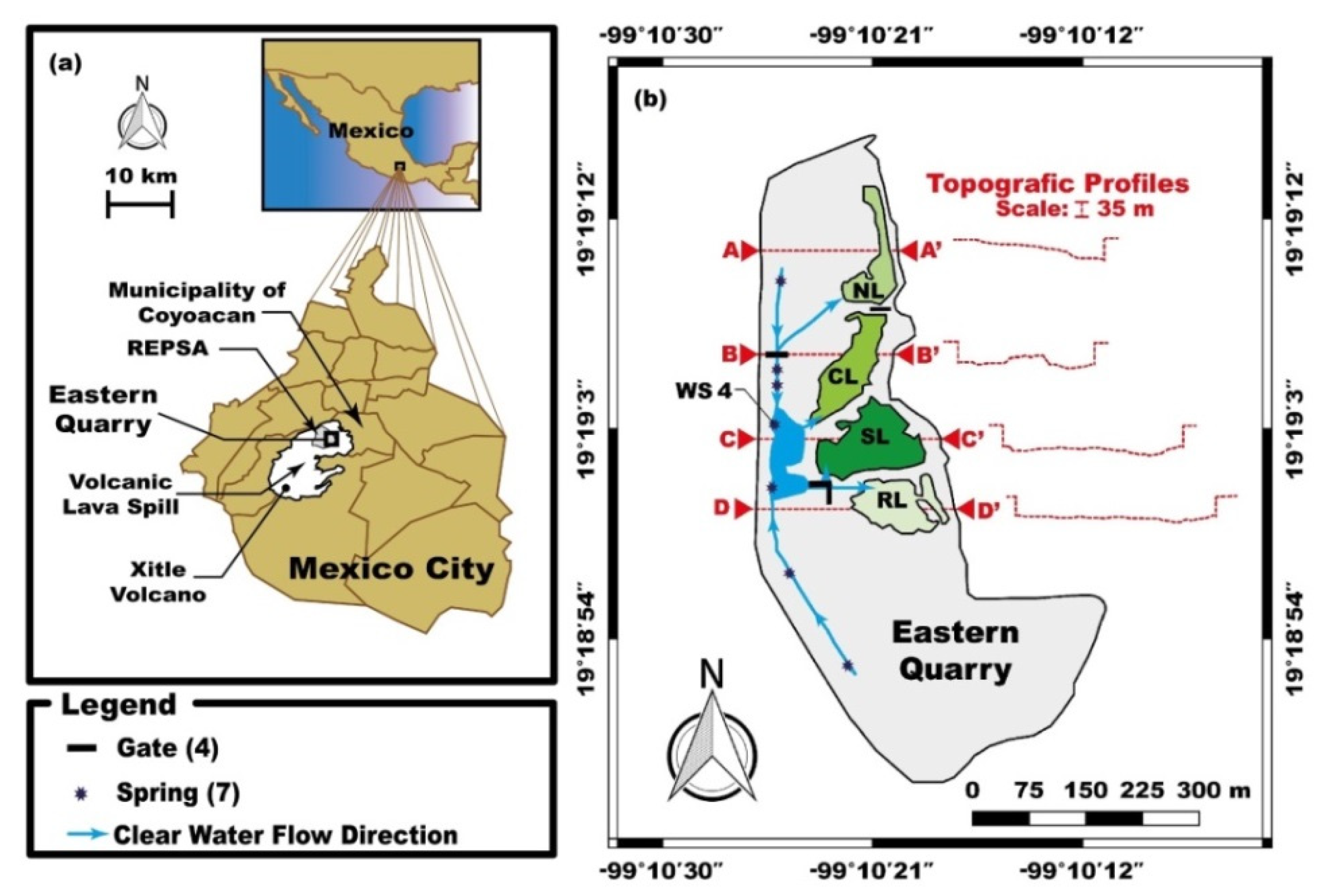
2.1. Study Site

The lakes are located within the Eastern Quarry (EQ) (Cantera Oriente, in Spanish; 19°19′15″–19°18′47″ N and 99°10′22″ W) within the Ecological Reserve of Pedregal de San Angel (REPSA), situated northeast of the Xitle volcano lava spill, whose extension is 80 km² (Figure 1a,b) [11]. The lakes are located within the EQ, which is part of the Ecological Reserve of Pedregal de San Angel (REPSA). This ecological urban reserve protects the last existing portions of vegetation that were very extensive in the past at Mexico’s basin, like the scrub of “Palo loco” (Pittocaulon praecox) [12].

The water that filled the EQ lakes came from the springs of a shallow aquifer flowing through the rocks (fractured basalt) along with the lava spill, as the main recharge sites of the shallow aquifer are the terrains near to the Xitle volcano [13], whose summit is 3100 m a.s.l. and is located 9.5 km southwest of the EQ [11] (Figure 1a).

The EQ has a total area of 206,000 m² divided into two areas. The northern part corresponds to the ecological reserve. From the D-D’ topographic profile to the southern end of the EQ (Figure 1b), the area is a training ground for a professional football team [12].

The EQ is a depression created due to the extraction of volcanic rock (basalt) during the period 1970–1994. The depression has an altitude range between 2254 and 2292 m a.s.l. [12]. Then, the lakes are classified as high-altitude water bodies, but are also tropical, considering the latitude [14]. The lakes originated when the excavation reached the aquifer and several springs appeared. EQ lakes approximately have the following surfaces, excluding flood zones: NL(5450 m²) < RL(6400 m²) < CL(8300 m²) < SL(9500 m²) [15].

The water flows through a series of channels to the different lakes. The water flow is regulated by gates (4), two of which are located near the mouths of the SL and the RL, with one in the channel, and another that divides NL and CL. The water leaves the shallow lake system area through two holes in the eastern wall—one located north of NL, and the other, most important one in RL. There is no sanitary network that discharges into the lakes; the wastewater is collected in septic tanks and treated later.

The climate in the EQ is temperate subhumid, with rains in the summer and a dry winter season; the rainy season lasted from May to October, and the dry season from November to April. The average annual rainfall is 833 mm, the average annual temperature is 15.6 °C, and predominant winds come from the north and NNE [12]. Over the studied period, September was the month with the highest monthly mean precipitation (127.4 mm), and February was the driest month (1.7 mm). In the period 2013–2016, the average rainfall in the dry season was 123.9 mm, while that in the rainy season was 490.9 mm [16].

The EQ water bodies fulfill the function of maintaining regional biodiversity. The presence of macrophyte vegetation is usually limited to the channels and the littoral zone of the water bodies, even in those water bodies that are more transparent, because it is continuously removed or trimmed. The main species of macrophytes living in the water bodies is Rush (Typha latifolia), and in the channels, the predominant species are the submerged plant, Sago Pondweed (Stuckenia pectinata) and the floating Swollen Duckweed (Lemna gibba) [17]. The species richness of phytoplankton in the water bodies of the EQ is 137, where chlorophytes (Scenedesmus, Desmodesmus, Actinastrum, Chlamydomonas) and bacillariophytes (Cyclotella, Gomphonema, Cymbella) present a higher number of species [18]. The lakes, in addition to the Common Carp (Cyprinus carpio), are inhabited by endemic species of the Valley of Mexico, such as the fish Mexclapique of Zempoala (Girardinichthys multiradiatus) [19] and Moctezuma’s Green Frog (Rana montezumae Baird) [20]. These lakes have also been used as a temporary shelter for the Mexican Ajolote (Ambystoma mexicanum) [21], and refugee area for several species of aquatic birds [22].

2.2. Sampling and Analysis of Water Parameters

Samples for the determination of the physical, chemical, and nutrient parameters of the lakes and the puddle were collected monthly from June 2013 to May 2016 (n = 36). The samples were integrated from the column every 0.2 m to the bottom.

All the water analyses were performed based on the protocols of the Standard Methods for the Examination of Water and Wastewater [23]. Water temperature (T), specific conductivity (K₂₅), and dissolved oxygen concentration (DO) were measured with a multiparameter YSI-85, the pH with a Conductronic PH-10 potentiometer, and the Secchi Disc depth (zSD) with a 20 cm diameter disc. Samples for determinations of Total Phosphorus (TP), P-PO₄³⁻, P-Org, Total Nitrogen (TN), N-NO₃⁻, N-NO₂⁻, N-NH₃, N-Org, CO₃²⁻, HCO₃⁻, Ca²⁺, and Mg²⁺ were kept at 4 °C until analysis in a maximum time of 24 h. The sample collected for the determination of Ca²⁺ and Mg²⁺ was added with HNO₃ (down to pH ≈ 2) as a conservative.

Standardization procedures and quality control gave recovery percentages of 95–99%, and coefficients of variation (CV) between 0.9% and 2.0% when replicates were obtained. Within the sampling period 2013–2016, Chl a was also determined with the acetone (90%) extraction method and read using a 10-AU Turner Designs fluorometer [24], and as quality control, tripled samples were analyzed in each batch, obtaining CV < 5%.

2.3. Trophic State Index (TSI)

The trophic state index of Carlson to estimate and classify the degree of eutrophication [25] uses three limnological parameters, such as Chl a (μg/L), zSD (m), and TP (μg/L) to calculate the Integral TSI (TSI-Int) according to the following equations:

$$\mathrm{TSI} \mathrm{Chl} \mathrm{a}=9.81\ln \left(\mathrm{Chl} \mathrm{a}\right)+30.6$$

(1)

$$\mathrm{TSI} \mathrm{zSD}=60-14.41\ln \left(\mathrm{zSD}\right)$$

(2)

$$\mathrm{TSI} \mathrm{TP}=14.42\ln \left(\mathrm{TP}\right)+4.15$$

(3)

$$\mathrm{TSI}-\mathrm{Int}=0.540 \mathrm{TSI} \mathrm{Chl} \mathrm{a}+0.297 \mathrm{TSI} \mathrm{zSD}+0.163 \mathrm{TSI} \mathrm{TP}$$

(4)

The Integral TSI (TSI-Int) was calculated with a modified formula that weighs TSI Chlor-a while reducing the weighting of TSI TP, because the availability of nutrients may not necessarily be the most important factor in promoting eutrophication (Equation (4)), and also to avoid overestimation of the values for classifying the trophic state, taking into account the relatively high TP values of the waters that feed the EQ [26].

The TSI-Int has a numerical scale of 0 to 100, and the values of the scale correspond to the different trophic states: 0 < TSI ≤ 30 oligotrophic, 30 < TSI ≤ 40 oligo-mesotrophic, 40 < TSI ≤ 50 mesotrophic, 50 < TSI ≤ 60 light eutrophic, 60 < TSI ≤ 70 medium eutrophic, and 70 < TSI ≤ 100 hyper-eutrophic [25].

2.4. Water Residence Time (WRT)

Theoretical or nominal WRT is defined by Equation (5), where V is the volume of the water body and Q is the daily flow in or out [27].

$$\mathrm{WRT}=\frac{\mathrm{V}}{\mathrm{Q}} \left(\mathrm{days}\right)$$

(5)

The WRT was estimated for each month and lake in the sampling period, except for WS 4 because it belonged to the channel network, but for statistical analysis and data management, at this site it was considered that WRT tended toward zero days. The average monthly volumes of lakes (V) were estimated from their surfaces and the monthly depths measured during the data collection period (2013–2016). To estimate Q, in each supply or output channel the surface velocity of the flow was measured using the float method, considering that the surface velocity is higher than the average flow rate. The use of a correction factor improves the estimation by this method. Finally, the velocity was multiplied by the area of the cross-section of the wetted perimeter of the different channels, then the Q estimated values were obtained [28].

2.5. Hydrogeochemical Modelling of Divalent Cations Minerals

Ca²⁺ and Mg²⁺ under certain conditions can form different minerals that remove PO₄³⁻ from the water column and attenuate eutrophication by precipitation or co-precipitation [29,30]. The saturation index (SI), defined as Equation (6), gives the potential formation of any solid in an aqueous medium:

$$\mathrm{SI}=\mathrm{Log}\frac{\mathrm{IAP}}{\mathrm{Kps}}$$

(6)

where IAP is the ionic activity product for the solid and Kps is the constant of the solubility product of the modeled solid. If SI < 0, the solid is dissolved; when SI = 0, the solid is in chemical equilibrium and can precipitate; and if SI > 0, the system is oversaturated and the solid can precipitate as well [31].

For the development of the hydrogeochemical models, the Aqion program was used, and the basis of this program was the method of calculating the thermodynamic balance that bases its numerical calculation on USGS Phreeqc [32]. The Aqion program offers the results of both SI and concentration of the solid that can potentially form (µM).

Hydrogeochemical models for the formation of phosphates with divalent cations were made for each month in the four lakes, and in WS 4 with the available variables of the 2013–2016 sampling period [Ca²⁺, Mg²⁺, CO₃²⁻, HCO₃⁻, pH, temperature (T), N-NO₃⁻ and P-PO₄³⁻], but due to not having the concentrations of all the major elements, the errors in the ion balances were completed with little or no reactive ions, such as Na⁺ or Cl⁻, according to the case.

For additional data handling of this parameter, as statistical analyses, the unit µM was used instead of SI values, since the SI may incorporate negative and zero values, making it difficult to find just a valid transformation factor for all other variables. In the case of the hydrogeochemical data that were not analyzed statistically, the SI values were used.

2.6. Organic Carbon in Sediments (OC)

The samples were taken from different sites at the bottom of the lakes in October 2017. The determinations were made by triplicate, through the oxidation method of the organic matter with potassium dichromate (K₂Cr₂O₇) and sulphuric acid (H₂SO₄) [33]. The method was standardized (n = 7) with anhydrous dextrose, obtaining a 99% recovery and 1.6% of CV.

2.7. Spatial and Temporal Differences in Water Parameters

The Discriminant Analysis (DA) was used to evaluate the spatial differences for the analyzed variables between the different water bodies, also allowing to define the contribution of each variable to the grouping of observations [34]. The data was transformed to n + 1, and then the Log₁₀ transformation was applied to minimize the biases of the data distribution, bringing them closer to a normal distribution [35]. The DA was performed with the XLStat 2014 program [36].

To figure out whether there were significant differences between the climatic seasons, a PERMANOVA analysis using PAST ver. 3.11 was performed [37]. Environmental data (Chl a and nutrients) for the rainy and dry seasons were previously transformed using n+1 and Log₁₀.

2.8. Partial Least Squares Regression (PLSR)

The PLSR is useful for solving multicollinearity problems in variables [38]. This study applies PLSR to identify the most influential variables on the trophic status for the studied lakes, considering Chl a as the modeled variable. PLSR models were implemented with the XLStat 2014 program [36], following the procedure proposed by Tenenhaus based on the retention of significant variables for the model, according to the β coefficients, confidence intervals, and with their contribution to explaining the variable response [39]. To improve model performance metrics, outlier data were removed, based on the Dixon test [40]. In the NL and CL models, no data were removed, while in the SL model, the three highest observations (outliers) were removed, and in the RL model, one outlier was removed.

2.8.1. Determination Coefficient (R²) and Stone–Geisser Index (Q²)

The value of R² is interpreted as the proportion of the variance of the dependent variable explained by the model [38].

The Q² is a jack-knife (cross-validation) version of R², which predicts the variation of the dependent variable [38]. The Q² index shows how the data omitted from cross-validation can be reconstructed with the help of the model and with the optimal number of PLS components, which include the response variable for its building [41]. If Q² > 0, the model has predictive relevance, while Q² < 0 suggests that the model lacks predictive relevance [42].

2.8.2. Root of the Mean Square Error of Prediction (RMSEP)

The mean square error of the prediction (MSEP) or its square root (RMSEP) is often used to evaluate regression performance; the minimum RMSEP value suggests the best model, so this parameter gives the criteria to choose the optimal number of components in PLSR [43], with the condition that the number of PLS components is less than the number of predictors [44]. If the choice of the optimal number of components is not adequate, the model can over-adjust R² in Q² demerit [39].

2.8.3. Significance and Importance of Variables in PLSR Models

According to the Tenenhaus procedure, the selection of significant variables by the confidence interval of the standardized coefficients, also called the β coefficients, is an iterative process in which from saturated PLSR models, they go away, discarding those variables whose confidence interval of the β coefficient includes zero on its range of values. This procedure is repeated as many times as necessary with the retained variables until no variable includes zero in the range of values of the confidence interval of the respective β coefficient [45]. Saturated models included all variables in

Table 1. Summary of environmental conditions (2013–2016).

Parameter	NL Mean ± SD (Min-Max)	CL Mean ± SD (Min-Max)	SL Mean ± SD (Min-Max)	RL Mean ± SD (Min-Max)	WS 4 Mean ± SD (Min-Max)
Depth (cm)	94 ± 17 (60–120)	118 ± 13 (100–150)	109 ± 16 (80–150)	121 ± 11 (100–140)	65 ± 14 (20–100)
WRT (days)	5 ± 5 (2–16)	9 ± 11 (2–31)	15 ± 14 (3–90)	3 ± 5 (1–9)	≈0
T (°C)	16.5 ± 1.7 (12.1–18.6)	17.5 ± 1.7 (13.4–19.8)	18.8 ± 1.8 (14.1–21.1)	17.8 ± 1 (14.9–19.5)	17 ± 0.6 (15.2–18.5)
K25 (µS/cm)	411 ± 33 (362–480)	398 ± 34 (331–472)	385 ± 23 (340–423)	400 ± 21 (358–452)	415 ± 35 (364–491)
Ca2+ (mg/L)	26 ± 4 (19–42)	26 ± 4 (17–40)	23 ± 3 (19–34)	24 ± 3 (21–36)	26 ± 4 (22–37)
Mg2+ (mg/L)	14 ± 3 (7–22)	13 ± 2 (6–19)	13 ± 3 (7–20)	14 ± 3 (7–19)	13 ± 3 (5–20)
CO32− (mg/L)	6 ± 32 (0–192)	37 ± 38 (0–160)	52 ± 29 (0–144)	5 ± 22 (0–128)	0 ± 0 (0–0)
HCO3− (mg/L)	75 ± 31 (32–184)	39 ± 27 (12–112)	22 ± 20 (2–72)	66 ± 26 (36–168)	67 ± 42 (32–256)
N-NO3− (mg/L)	4.7 ± 1.1 (2.1–6.5)	4.6 ± 0.9 (2.4–6.3)	4.4 ± 1.3 (1.9–8.8)	7.2 ± 1.3 (2.9–9.1)	7.3 ± 1.4 (3.7–10.4)
N-NO2− (mg/L)	0.03 ± 0.2 (0.01–0.12)	0.05 ± 0.02 (0.01–0.13)	0.09 ± 0.04 (0.02–0.18)	0.03 ± 0.02 (0.01–0.13)	0.01 ± 0.01 (0.01–0.07)
N-NH3 (mg/L)	0.08 ± 0.05 (0.01–0.23)	0.07 ± 0.06 (0.01–0.27)	0.07 ± 0.05 (0.01–0.25)	0.02 ± 0.02 (0.01–0.09)	0.03 ± 0.03 (0.01–0.17)
N-Org (mg/L)	1.7 ± 1.3 (0.2–4.9)	2.7 ± 2.1 (0.3–8.8)	3.4 ± 1.9 (0.3–9.5)	2.0 ± 1.7 (0.1–6.3)	2.5 ± 2.3 (0.1–11.2)
TN (mg/L)	6.6 ± 1.3 (4.5–11.8)	7.9 ± 3.2 (5.1–22.2)	8.3 ± 2.7 (5.1–18.6)	9.9 ± 3.5 (6.6–28.1)	11.1 ± 7.5 (6.1–52.7)
P-PO43− (mg/L)	0.10 ± 0.4 (0.05–0.25)	0.08 ± 0.07 (0.01–0.35)	0.05 ± 0.05 (0.01–0.25)	0.13 ± 0.07 (0.06–0.38)	0.13 ± 0.03 (0.09–0.25)
P-Org (mg/L)	0.05 ± 0.03 (0.02–0.11)	0.12 ± 0.09 (0.02–0.42)	0.12 ± 0.16 (0.01–0.97)	0.06 ± 0.06 (0.01–0.29)	0.03 ± 0.03 (0.01–0.15)
TP (mg/L)	0.21 ± 0.13 (0.10–0.55)	0.19 ± 0.13 (0.05–0.58)	0.17 ± 0.16 (0.06–1.03)	0.18 ± 0.12 (0.09–0.58)	0.18 ± 0.10 (0.10–0.52)
P-HAP (mg/L)	0 ± 0 (0–0)	0.033 ± 0.026 (0–0.14)	0.006 ± 0.007 (0.001–0.035)	0 ± 0 (0–0)	0 ± 0 (0–0)
TN:TP (by mass)	39 ± 16 (13–63)	49 ± 18 (14–84)	69 ± 37 (10–199)	67 ± 23 (14–120)	62 ± 20 (18–133)
Chl a (µg/L)	57 ± 39 (7–147)	131 ± 80 (16–336)	162 ± 120 (39–622)	21 ± 16 (4–63)	6 ± 8 (1–36)
zSD (cm)	77 ± 19 (45–120)	54 ± 23 (20–120)	37 ± 14 (8–80)	112 ± 16 (65–140)	61 ± 11 (43–100)
DO (mg/L)	9.4 ± 3.1 (5–17.2)	14.1 ± 4.9 (6–23.3)	17 ± 4.7 (5.3–25.3)	12.9 ± 4.2 (7.9–28.4)	6.8 ± 1.7 (4.8–13.5)
pH	7.4 ± 0.5 (6.7–9.0)	8.3 ± 0.5 (7.2–9.7)	9.0 ± 0.4 (8.1–10)	7.8 ± 0.6 (6.9–9.9)	7.3 ± 0.4 (6.6–8.6)
TSI-Int	69 ± 5 (60–77) Medium Eutrophic	75 ± 5 (63–83) Hyper Eutrophic	77 ± 5 (66–88) Hyper Eutrophic	61 ± 4 (52–73) Medium Eutrophic	57 ± 5 (48–68) Light Eutrophic

, except TSI-Int, mainly because it is an index derived from Chl a (Equation (4)).

The variable importance in projection (VIP) values derived from loads of the β coefficients summarizes the relative importance of the predictors in the PLSR model, and provide a useful measure in the selection of variables that contribute most to the explanation of the variance of the dependent variable [46]. The VIP values for considering a moderately influenced variable are 0.7–0.8 < VIP < 1, and to classify the influence of a variable as “high”, the VIP must be higher than 1 [47].

3. Results

3.1. Environmental Conditions in the Lakes (2013–2016)

Table 1 shows a summary of the results of the variables analyzed during 2013–2016. The average depth of the lakes varies between 94 and 121 cm. WS 4 is a part of a channel that has an average depth of 65 cm, with extreme values of 20–100 cm in the sampling site; however, the five sites show a relatively low standard deviation (SD) between 11 and 17 cm, probably due to the dampening of flood zones. Among the sites studied, it is remarkable that the flow of water supply of RL was higher than that of the other lakes, so the WRT for RL was lower (RL < NL < CL < SL). Differences in WRT may be due to the operation of the hydraulic lake infrastructure that varies depending on the season of the year (rainy or dry seasons), and the requirements of maintenance or sports activities that take place in the EQ.

The maximum and minimum WRT values are probably associated with the rainy and dry seasons, because the water of the springs comes from a shallow aquifer composed of high hydraulic conductivity materials, as fractured basalt. It was observed that over a few days (approximately 7–15), the flows of the springs reflected notorious changes according to the season. The flow value in one of the springs was almost 80 m³/day in the dry season, and almost 10,200 m³/day in the rainy season [13].

The operation of the gates is decisive in the distribution of water and on the WRT values. During the rainy season, as far as possible, the gates work to avoid flooding of the lowest areas in EQ, and in the dry season, to avoid an excessive drop in lake level. Therefore, seasonal effects can be partially masked by gate management.

The average temperature in the water column exhibits the following order: NL < WS 4 < RL < CL < SL. NL, CL, and mainly SL have remarkable dispersion values (>1.0 °C), while RL and WS 4 have SD values less than 1 °C, which may be explained by the difference in the exposure of lakes to sunlight due to the adjacent rock wall that is 30–38 m high (Figure 1).

The K₂₅ shows the average maximum values in WS 4 and NL; both sites also exhibit the highest dispersion in the data along with the CL, while the RL and SL show the lowest SD values. The lowest average values of K₂₅ in CL, SL, and RL may be associated with solid precipitation.

The Ca²⁺ reveals very similar average values in all water bodies (23–26 mg/L) and SD around 3 mg/L, as does Mg²⁺, but the latter exhibits average values in the range of 12.6–13.6 mg/L. These elements probably come from the weathering of non-calcareous minerals [48].

Concerning alkalinity, CO₃²⁻ had changing values in the different shallow lakes ranging from 0.0 to >100 mg/L, except WS 4, which presented with 0.0 throughout the sampling series. HCO₃⁻ is the predominant ion in alkalinity and exhibited significant variations in results at each of the sites studied, including WS 4 (20–256 mg/L).

The carbonated ions in waters that cross basaltic substrate (low alkaline reserve) probably come from the soil area where the water infiltrated; decomposition of organic matter, the action of the roots, and the microbial respiration generate a CO₂ concentration of one or two orders of magnitude higher than the concentration of CO₂ in the air, and based on pH, it transformed into HCO₃⁻ or CO₃²⁻ [49].

As for nutrients, N-NO₃⁻ is the most abundant analyzed nitrogen ion in the system (SL < CL < NL < RL < WS 4), covering a range of concentrations between 1.9 and 10.4 mg/L. The N-NO₂⁻ has an average concentration range between 0.01 and 0.09 mg/L, following the reverse order of N-NO₃⁻, with SL having the highest concentration associated with WRT [50]. The N-NH₃ in the different shallow lakes exhibit the following average concentration series: RL < WS 4 < CL < SL < NL, in a range of 0.02–0.08 mg/L, while the series for N-Org is NL < RL-WS 4 < CL < SL, with average values of 1.7 to 3.4 mg/L.

The ion with the greatest contribution to TN is N-NO₃⁻ (WS 4 < RL < SL < CL < NL). The order of concentration may be associated with consumption of N by phytoplankton and abundant macrophytes residing in the channel network, as N is also the most required nutrient for macrophytes. Besides, the NL waters are the ones that travel the longest distance through the channels, followed by the waters of CL and SL, respectively (Figure 1b).

For phosphorus, the average concentrations of P-PO₄³⁻ (SL < CL < NL < RL-WS 4) have values between 0.05–0.13 mg/L, where RL and WS 4 have similar concentrations, probably due to lower phytoplanktonic consume. P-Org (WS 4 < NL < RL < CL < SL) exhibits a range between 0.03 and 0.12 mg/L, which may also be related to the abundance of primary producers.

RL and WS 4 present equal values of TP, although SL, CL, and NL present light deviations probably associated with the activity of the primary producers or chemical processes.

TN:TP ratios were calculated by mass, showing a range between 10 and 199 (CL < NL < RL < WS 4), and averaging (57 ± 23), this value suggests that P is the limiting nutrient in accordance with the Redfield ratio (7.2 by mass) for phytoplankton. However, the effect of the TN:TP ratio depends on the concentration of P and N [51]. High TN:TP values and high concentrations of TP can generally relieve the P deficiency and allow for significant phytoplankton growth, as evident in the lakes of the EQ [52].

According to hydrogeochemical models, the only phosphate compound that had SI > 0 was HAP [Ca₅(PO₄)₃(OH)]. The P-fraction was calculated in the HAP (P-HAP). This mineral is perhaps the most crucial calcium phosphate compound for all uses and applications [53]; it has low solubility and may form under certain conditions that are present in EQ lakes (enough concentration of Ca²⁺ and PO₄³⁻, adequate temperature values and increases in pH values, due to primary production). These conditions favor the formation of the mineral, which would remove PO₄³⁻ from the water column and thereby reduce eutrophication [29].

P-HAP results show that NL, RL, and WS 4 did not offer conditions for HAP formation and, therefore, for the presence of P-HAP. In CL and SL, the conditions for the potential formation of HAP were presented because they are warmer and have higher pH values caused by eutrophication, which promotes the formation of this mineral in less time. However, the HAP concentration in CL is about 5.5 times higher than in SL, as the latter lake has the lowest concentration of P-PO₄³⁻ due to the high consumption by primary producers.

Variables influenced by eutrophication, such as DO concentration, deploys the series: WS 4 < RL < NL < NL < CL < SL, while zSD reversely exhibits the same series as DO. Note that the depth and zSD in both RL and WS 4 are similar, as in most measurements, the depth was equal to zSD. Concerning pH, the order of values remains WS 4 < NL < VL < RL < CL < SL.

Chl a has the same order of values as DO, which also has consistency with the TSI-Int results, where NL is referred to as “medium eutrophic”, just like RL, while CL and SL are hyper-eutrophic and WS 4 is light eutrophic. In some cases, when zSD = depth, the TSI zSD contribution overestimated the TSI-Int values mainly with regard to WS 4 and RL, where the zSD = depth condition is displayed in 36 and 30 cases, respectively.

The various trophic state conditions of these shallow lakes are probably associated with the differences that most variables present in the sites studied, reflecting different interactions between the environmental variables. As can be seen in RL and WS 4, where the predominant trophic condition is light eutrophic, they are possibly associated with the short WRT of WS 4.

Calcite is a solid that can be formed according to pH [54].

Table 2. Saturation index (SI) for calcite.

pH	NL SICalcite	CL SICalcite	SL SICalcite	RL SICalcite	WS 4 SICalcite
Mean ± SD 1	−1.30 to 0.49	0.22 to 1.13	0.99 to 1.59	−0.42 to 0.88	−0.77 to 0.10

¹ The pH values (Mean ± SD) correspond to the data calculated in the 2013–2016 results series.

shows calcite saturation rates (SI_Calcite) in the lakes and that are based on pH. Conditions for calcite formation in NL, RL, and WS 4 are not favorable most of the time, and can only be seen as favorable when pH values are high; CL and SL show adequate conditions for the potential calcite formation in the respective range. The limited calcite formation can be explained by the reduced formation of carbonic acid, since primary producers take advantage of dissolved CO₂ for photosynthesis, and this raises the pH, promoting the transformation of HCO₃⁻ into CO₃²⁻ [55].

The organic carbon concentrations (OC) of sediments in the shallow lakes (

Table 3. Organic carbon (OC) in the sediments.

Parameter	NL	CL	SL	RL	WS 4
OC (%)	11.75 ± 0.12	4.37 ± 0.10	1.96 ± 0.09	3.09 ± 0.10	Not Measured

) differ (SL < RL < CL < NL); however, the concentration of OC in the sediments in the NL is significantly higher than at other sites. Primary producers can generate the OC, and in the case of NL, the highest value could relate to the inputs from the adjacent hillside with abundant plant cover (Figure 1).

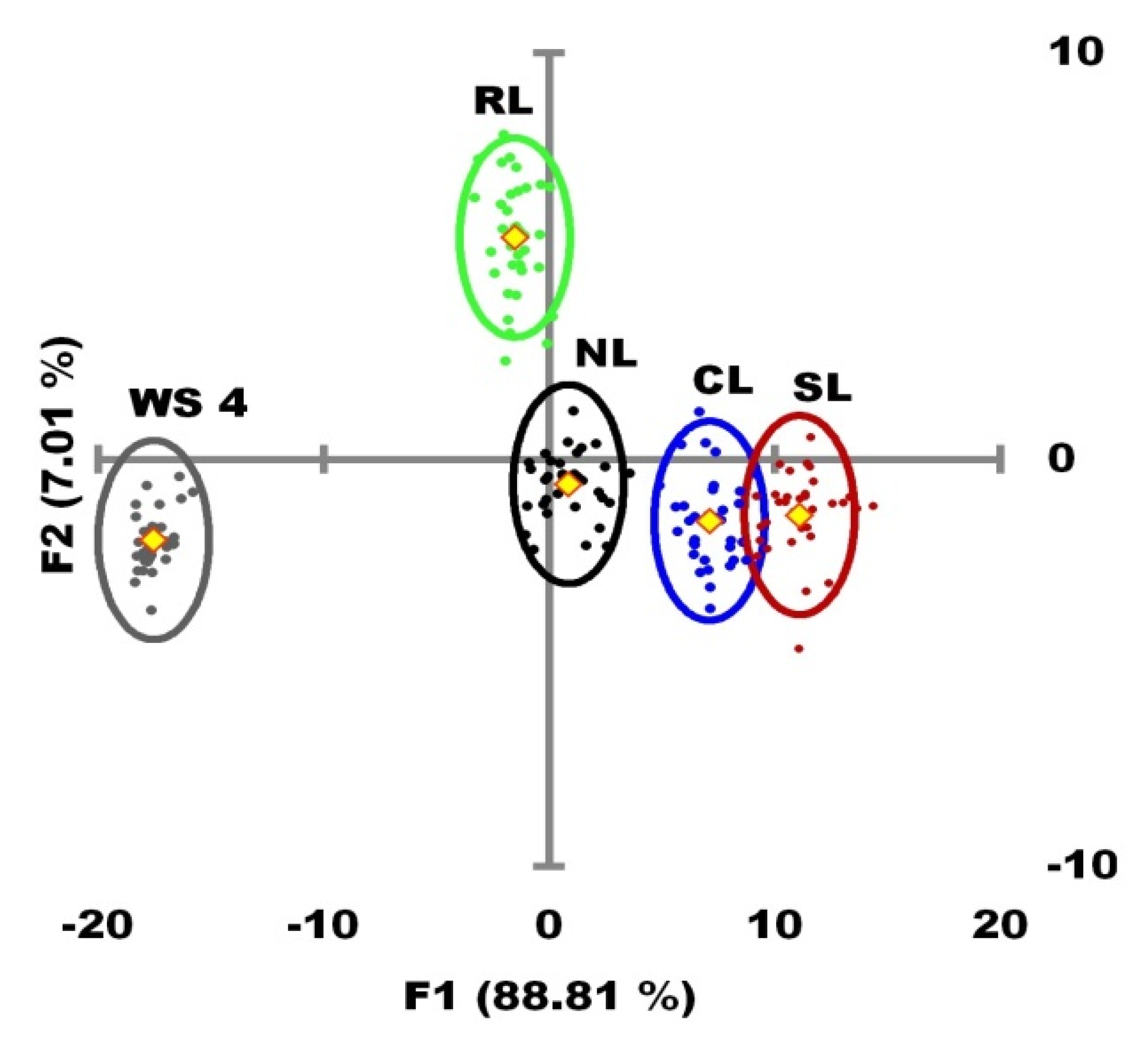
3.2. Spatial and Temporal Differences in Water Parameters

In order to establish the differences between the water bodies studied, a DA was performed.

Table 4. Correlations with discriminating functions.

Parameter	F1	F2
K25	−0.295	−0.012
DO	0.695	0.147
pH	0.755	−0.104
Chl a	0.866	−0.214
zSD	−0.341	0.691
Ca2+	0.021	−0.918
Mg2+	−0.067	0.786
CO32−	0.682	−0.360
HCO3−	−0.429	0.248
N-NO3−	−0.578	0.429
N-NO2−	0.625	−0.207
N-NH3	0.341	−0.271
P-PO43−	−0.487	0.186
P-Org	0.387	−0.141
WRT	0.997	−0.022
Variance Explained	88.81%	7.01%
Wilk’s lambda	<0.001	0.014
p-value	<0.001	<0.001

Significant correlations in bold.

presents the variables with the highest correlation with the first two discriminating functions; these correlations allow for the influence of the different variables in the classification to be measured.

The F1 discriminating function explains 88.81% of the variance, and F2 explains 7.01%; both functions are significant, as shown by Wilk’s Lambda and the p-value. F1 concentrates the values of the highest coefficients of K₂₅, DO, pH, CO₃²⁻, HCO₃⁻, nitrogen, and phosphate ions, WRT and Chl a, while F2 correlates with zSD, Ca²⁺, and Mg²⁺.

The variable with the most influence on group discrimination is WRT, which presents a high correlation with the explanatory function of variance (F1).

Figure 2 illustrates the results of the DA; WS 4 and RL were different from the other lakes, and did not share characteristics among them. NL and RL showed a greater proximity to WS 4, while the SL and CL point clouds were present. NL and RL showed greater proximity to WS 4, while the SL and CL point clouds presented with an incomplete overlap, as both lakes have been classified in the same category in the TSI-Int (hyper-eutrophic), although they may have some differences.

The PERMANOVA analysis was applied using the Chl a and nutrients and did not show differences (p > 0.05) between the dry and rainy seasons.

3.3. Identification of Key Factors in the Trophic State by PLSR

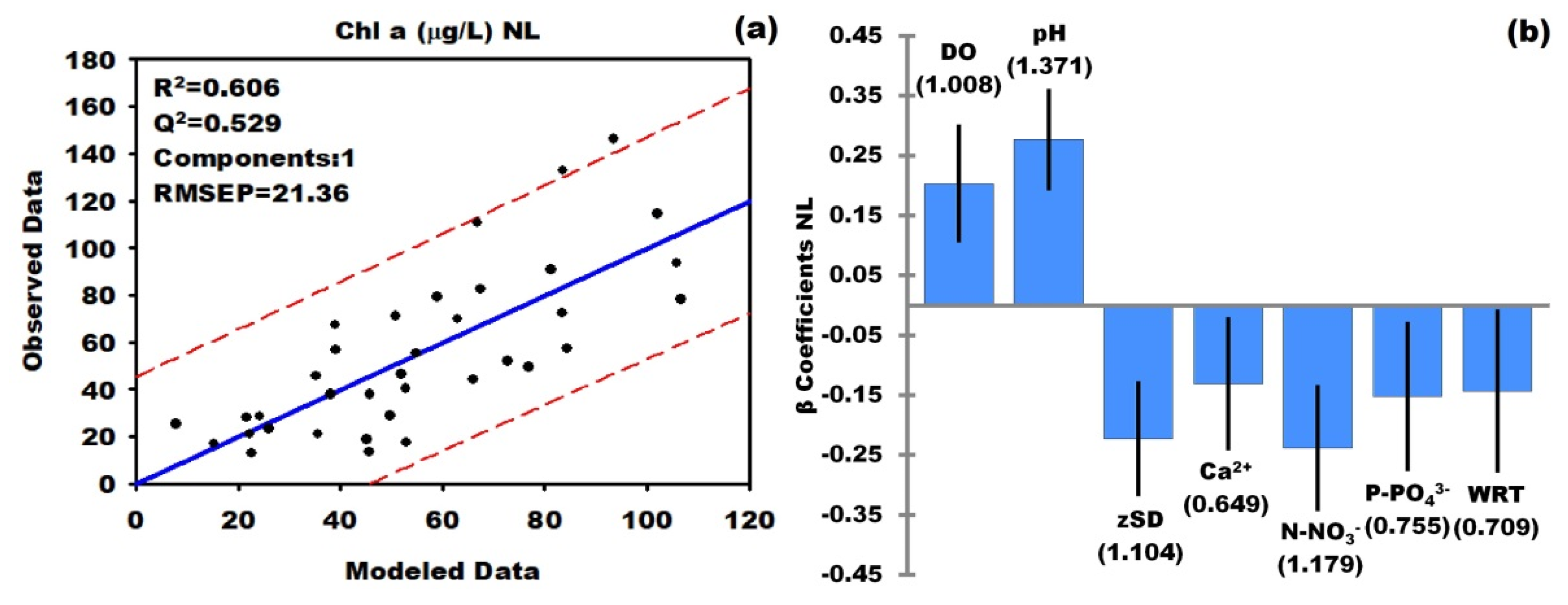
3.3.1. North Lake (NL)

Figure 3a presents the scatter plot and performance metrics of the model, while R² explains 60.5%, and Q² predicts 52.9% of the Chl a variation. The model with one PLS component had the lowest RMSEP value.

On the Y-axis (Figure 3b), the positive values of the β coefficients for DO and pH reflect direct relationships of the predictor variables modified by eutrophication with Chl a; the negative values of the β coefficients of the rest of the variables indicate inverse relationships.

The VIP value (Figure 3b) indicates that the variables modified by eutrophication (pH, zSD, and DO) are the ones that bring the most weight to the model, as well as N-NO₃⁻. The WRT and P-PO₄³⁻, have moderate influence, while Ca²⁺ has a minor influence on the model, but is significant, based on the β coefficient confidence interval. Variables such as pH, zSD, and DO have a strong influence on Chl a modeling due to the variables that are directly affected by eutrophication.

Nutrients are recognized factors of eutrophication, so the VIP is moderate to high. The inverse relationship of the nutrients (N-NO₃⁻ and P-PO₄³⁻) with Chl a may be associated with consumption by primary producers, which contributes to the reduction in concentrations of dissolved nutrients in the water column.

After nutrients, WRT in NL is the most influential variable in the trophic state. The WRT in the EQ has a close relationship with the dry and rainy seasons: in the NL, the condition Up Chl a/Down WRT may occur, associated with the connection between NL and CL during the rainy season when the NL receives CL water with a higher Chl a load. The other condition is Down Chl a/Up WRT, and may be related to the non-connection of shallow lakes during the dry season, in addition to the reduction of temperature, photoperiod, and irradiance during the winter, which could contribute to a decrease in the activity of primary producers.

The inverse relationship of Up Chl a/Down Ca²⁺ is probably associated with the NL, sometimes having positive SI_Calcite values (Table 2). The Down Chl a/Up Ca²⁺ relationship is feasibly associated with the water renewal (flushing) that replenishes the precipitated ions and dilutes the Chl a.

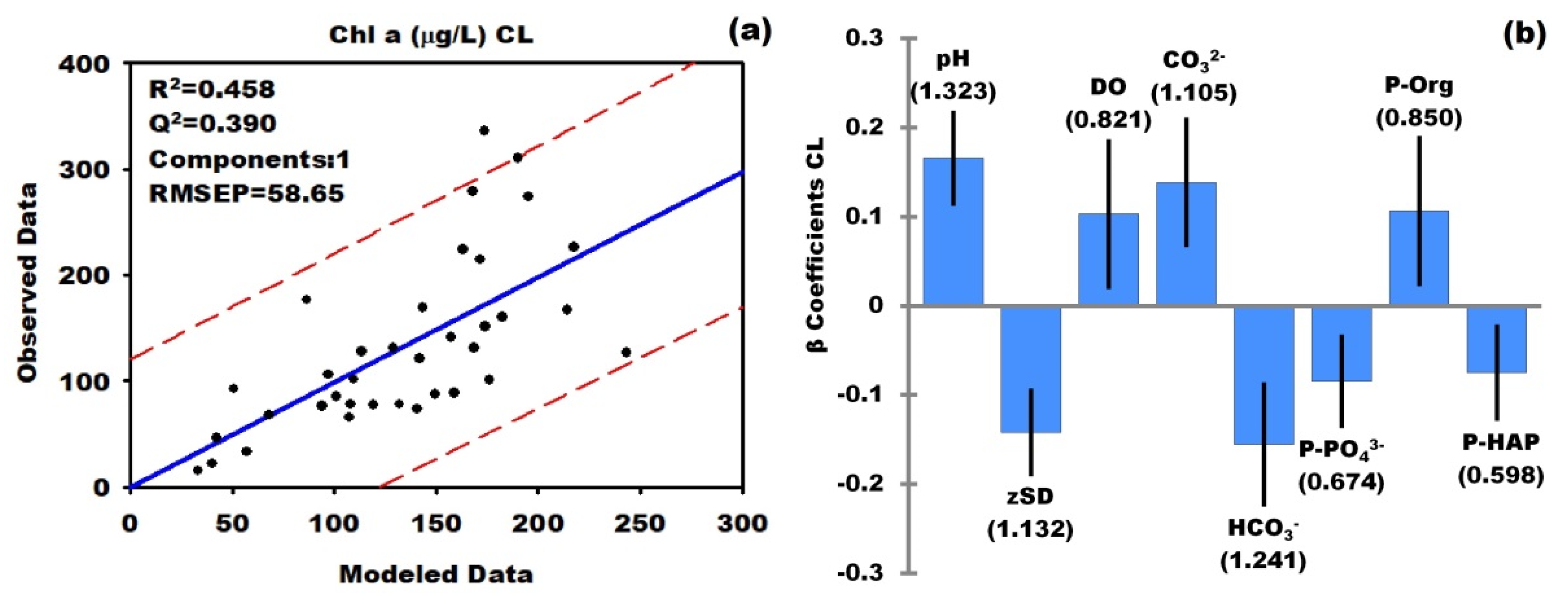
3.3.2. Central Lake (CL)

Figure 4a presents the scatter plot and performance metrics of the model, where R² explains 45.8% of the variance, and Q² predicts 39% of the Chl a variation. This model was built with one PLS component, and resulted in the lowest RMSEP value. Figure 4b shows the β coefficients of the retained variables and the confidence intervals of the β coefficients to check the significance of the variables. In this case, the signs of the β coefficients exhibit direct relationships with pH, DO, CO₃²⁻, and P-Org and inverse relationships with zSD, HCO₃⁻, P-PO₄³⁻, and P-HAP.

The variables that are modified by eutrophication (pH, DO, and zSD) and P-PO₄³⁻ have VIP values that classify them as variables of considerable influence, except for P-PO₄³⁻, which is low (VIP = 0.674), but the roles of these variables have already been mentioned and are not different from one lake to another.

HCO₃⁻ and CO₃²⁻ have a significant influence on the model (VIP > 1). Its high VIP values are associated with the modifications to pH generated by primary producers; however, in the case of CO₃²⁻, it is not discarded as a possible eutrophication attenuation factor because it could co-precipitate with P-PO₄³⁻ [30], due to CL presenting with SI_Calcite > 0 (Table 3).

The P-Org presented a direct relationship with Chl a of moderate influence in CL (VIP = 0.850), probably due to living and detrital organic matter. The CL presents the highest concentration of P-Org even without being the most productive site, which can be associated with the water movement that favors the accumulation of materials because it presents an orientation in which the north and NNE winds exert a movement of surface water in the opposite direction to the hydraulic gradient. In CL, the winds generate a slowdown, sufficient to probably cause the retention of P-Org in the water body.

The potential HAP formation can be a eutrophication attenuation factor, although the influence of this variable on the model is low (VIP = 0.598). The potential formation of HAP is considered as a possible attenuator because the average P-HAP concentration (0.033 mg/L) approximately corresponds to 25% of the mean P-PO₄³⁻ concentration (0.13 mg/L) in the waters supplying lakes from WS 4 (Table 1).

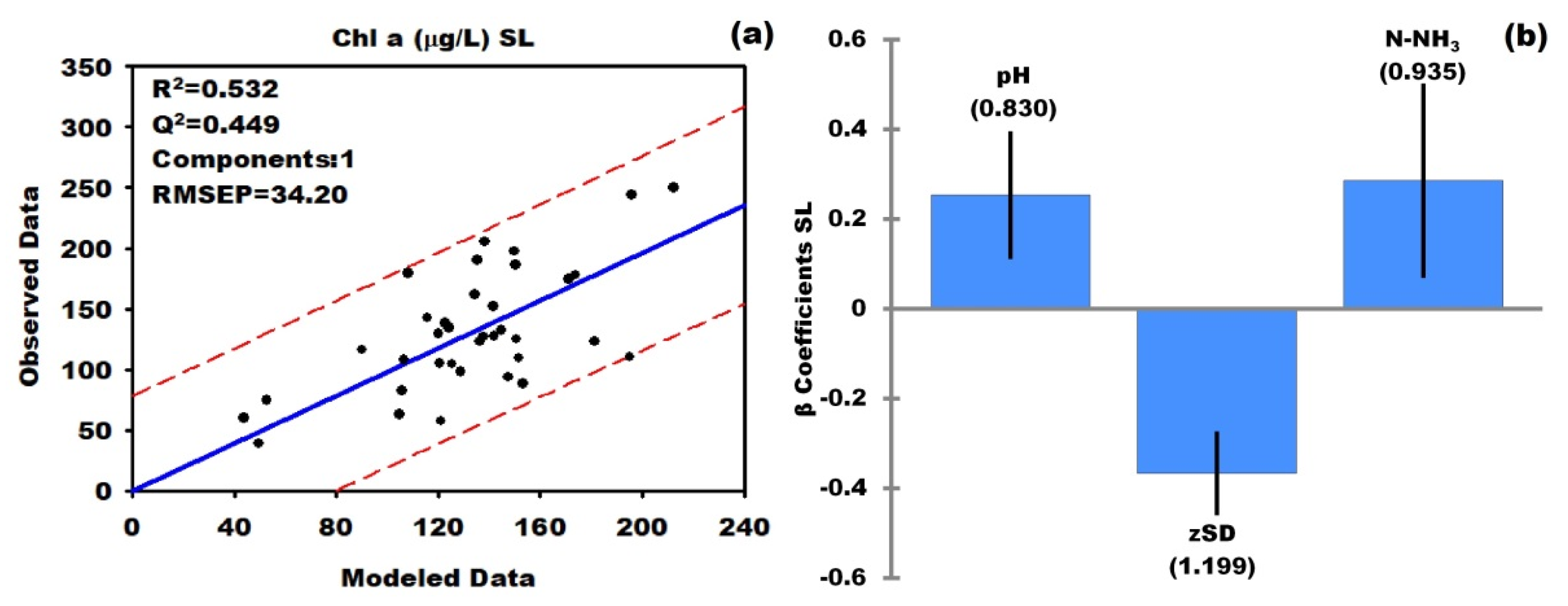
3.3.3. South Lake (SL)

In the SL model, R² explains 53.2% of the variance, and Q² predicts 44.9% of the Chl a variation (Figure 5a). The minimum RMSEP value was obtained with one PLS component.

The pH, and particularly zSD, are variables that strengthen the model performance metrics due to their VIP values (Figure 5b). The β coefficient of N-NH₃ has a significant direct influence on the model (VIP = 0.935), and this parameter may reflect a nutrient recycling process because the direct relationship N-NH₃/Chl a suggests that organic matter is decomposing, since ammonium is the dominant nitrogen ion at the beginning of the mineralization of organic matter [56]. Nutrient recycling or mineralization may be taking place in the water column, which is consistent with the lowest OC value in SL sediments (1.96%) (Table 3).

Additionally, SL being the warmest water body between EQ lakes can promote mineralization because it increases the activity of decomposers and related microorganisms [54], and the DO content in the SL water column is much greater than 2 mg/L, which is optimal for the removal of organic materials by biodegradation [57]. The direct relationship between N-NH₃/Chl a can also be explained by the ammonium that may be being used as a nitrogen source by primary producers and generate more chlorophyll [58].

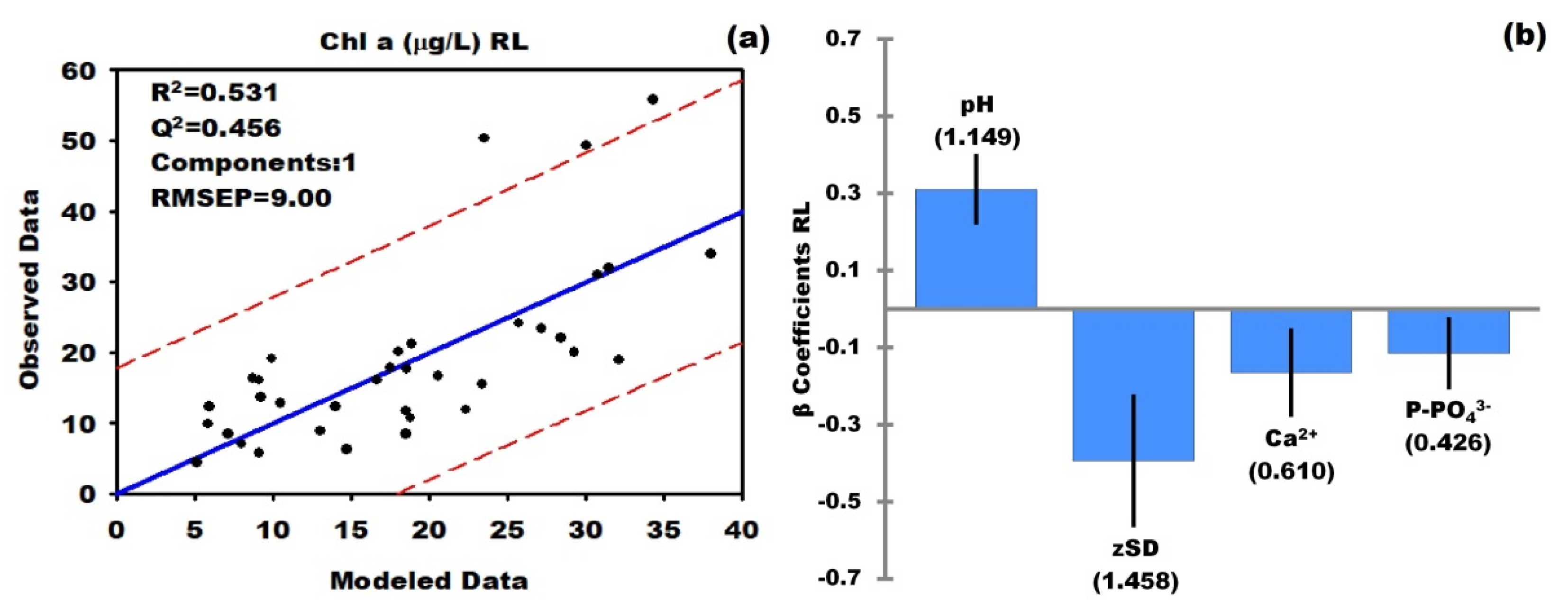
3.3.4. Regulation Lake (RL)

In the model, R² explains 51.5% of the variance, and Q² predicts 43.4% of the Chl a variation (Figure 6a). The minimum RMSEP value was obtained with one PLS component. The influence of pH and zSD, as on the other models, is evident (VIP > 1), followed by Ca²⁺ and P-PO₄³⁻ with low influences (VIP > 0.7), but is significant based on the confidence intervals of their respective β coefficients (Figure 6b). When the inverse relationships of Ca²⁺ and P-PO₄³⁻ with the Chl a have the condition Down Chl a/Up Ca²⁺ and P-PO₄³⁻, it is probably associated with flushing derived from WRT because RL has the lowest WRT among all the water bodies (3 ± 1 day) (Table 1), but the WRT is not among the significant variables, probably due to the delay in the response of the lake to the replacement.

In the condition Up Chl a/Down Ca²⁺ and P-PO₄³⁻, the reduction of Ca²⁺ can be associated with SI_Calcite > 0 (Table 2), and the inverse relationship Chl a/P-PO₄³⁻ may be associated with consumption of primary producers since HAP (Table 1) is not formed in this lake.

4. Discussion

The variances explained from Chl a in this study with PLSR (R² = 45.8–60.6%) are consistent with the results found in another tropical system, the lakes of the Paraná River basin in Brazil (R² = 52%) [59], strengthening the suggestion that linear regression models are useful tools for understanding the complex dynamics of the factors that compose the aquatic systems [59,60,61].

The presence of N-NO₃⁻ in EQ spring water may be due to edaphologic processes that start at the point where water infiltrates into the aquifer. N-NO₃⁻ concentrations in EQ springs, in general, do not exceed the limit for drinking water in Mexico [62]. Another previous study focused on analyzing wells within the borders of the lava spill, and its surroundings did not find concentrations higher than 10 mg/L of N-NO₃⁻ [63], suggesting that the water sprouts from the springs are not polluted with sewage.

The origin of P-PO₄³⁻ in the spring water can be lithogenic because the variation in WS 4 is low (±0.03 mg/l), which points to a stable and constant contribution over the sampling period, and because the phosphorus content in the basalts of Xitle volcano lava spill, such as P₂O₅, is 0.25–0.76% (1090–3320 mg/kg as P) [64]. These values are above the upper Earth crust value (757 mg/kg as P) [65]. The spill rock of the Xitle volcano, also rich in iron, aluminum, titanium, and manganese [64], is a basalt mostly composed of olivine and pyroxene [66], the olivine being one of the most reactive minerals in the presence of water [67], and the weathering of these minerals probably result in the release of PO₄³⁻ contained in the rock to the water that supplies the EQ lakes.

The nitrogen and phosphorus intake, primary production, and chemical processes of EQ are likely to be the origins of the high TN:TP ratios at EQ lakes (57 ± 23 by mass), which may be determining the phytoplankton community composition due to the TN:TP ratio. This ratio has a strong influence on biological structure and function, and is therefore widely used to handle and infer the phytoplankton community composition [68]. At low TN:TP ratios, cyanobacteria become dominant [68], and around 7.2 by mass at high N and P concentrations are optimal for Microcystis aeruginosa [51]. The average values of TN:TP ratios in EQ lakes are much greater than 7.2, and thus are able to explain why the dominant group of phytoplankton, in general, is not cyanobacteria, but chlorophytes and bacillariophytes, as mentioned above [18]. These are less harmful for the environmental condition of EQ water bodies.

In NL, nutrient consumption has a significant influence over the trophic state, so the identification of other variables that also participate in the expression of a particular trophic state is important. In NL, we found the WRT had an inverse relationship with Chl a. The WRT has been reported as a variable that relates directly to the increase in primary producers [69], which makes it relevant to focus on the type and response time of small and shallow water bodies.

The extraction of PO₄³⁻ from the water column as calcium compounds has been studied as a way to mitigate eutrophication [70], although the potential formation of HAP in CL is questionable for at least two reasons—firstly, because it may be affected by the relatively slow formation of the mineral. The formation kinetics may determine the concentration of PO₄³⁻ available for primary producers, without neglecting how the presence of humic substances inhibits HAP precipitation [71]; and secondly, because the CL model has the lowest PLSR (R² and Q²) performance metrics among the four models, and P-HAP also has a minor influence (VIP = 0.598). The pH of the spring water generally does not favor HAP precipitation, and it is only when the water resides in CL and the primary producers modify the pH when the conditions for the presence of HAP improve. However, due to the slow kinetics of HAP precipitation, primary producers are more likely to take advantage of PO₄³⁻ before HAP formation.

In our study, calcite was used to explain the removal of Ca²⁺ from the water column, and it was also able to participate in the co-precipitation of CaCO₃/PO₄³⁻, a process that has been reported as a mitigation factor for eutrophication in many lakes of different temperate areas of the world [30,72,73]. Co-precipitation has not been studied in depth under the conditions offered by CL (shallow tropical lake at high altitude), where there could be a minor attenuation factor. Co-precipitation depends on the initial concentration of PO₄³⁻—at low or high concentrations, the co-precipitation may below, or even inhibited. The high average concentration of P-PO₄³⁻ in CL (0.08 mg/L) would be an unfavorable condition for adequate co-precipitation rates [36].

Organic matter mineralization maintains its primary production in SL. A similar process occurred in four shallow eutrophic lakes with a limited external P load, where the organic matter decomposition was stimulated by rises in temperature, derived from a eutrophic state, but was also helped by the contributions of the phosphorus released from the aerobic surface of the sediment [74]. The ortho-phosphate ion, negatively charged, is electrostatically repelled by minerals in the sediment as oxides and hydroxides of iron, aluminum, titanium, or manganese when the water pH value in EQ lakes (6.6–10) could be higher than the pH values of the Points of Zero Charge of these minerals [75], which are present in the basaltic rock of the Xitle spill that presumably gave rise to the sediments of the EQ water bodies [64]. Additionally, in the sediments of eutrophic water bodies, lower concentrations of P-Org were found relative to others with a lower degree of eutrophication, suggesting that the decrease in P-Org concentrations is a consequence of the mineralization [76], a situation that was observed in SL but with the OC.

Often, the shallow lake sediments present a significant interaction with most of the water column, which can lead to mineralization if the water contains a sufficient amount of DO to satisfy the Sediment Oxygen Demand (SOD) [77,78], >2 mg/L, as mentioned above. Eutrophic lakes have a high amount of bacteria and other microorganisms as flagellates and ciliates, related to the abundance of organic matter, and all these organisms play a fundamental role in organic compound degradation [54], where the cilliates showed the highest abundance in SL [79]. In this lake (SL), due to the lower water supply (highest WRT), mineralization seems to be the process that supplies nutrients for eutrophication.

The rate of water renewal or flushing has been widely studied as a strategy for the remediation of all types of epicontinental water bodies, such as estuaries, lakes, rivers, reservoirs, and shallow lakes [80,81,82,83]. In EQ, flushing is applied due to the regulating function of the RL that dampens the flow rates coming from the springs to prevent flooding, dislodging the water as quickly as possible.

With the application of PLSR, not only were the most influential variables in the trophic state of each water body identified, but they also began with the knowledge of the processes present, in which the variables participated. The WRT is a variable that modifies chemical, physical, and biological aspects [10]. In NL, WRT had an apparent direct influence on the Chl a PLSR model; however, in the rest of the lakes, the influence of WRT could be considered indirect, due to the variables identified as influential on the processes that may be favored by the WRT, such as the possible attenuation of eutrophication by the potential formation of HAP in CL, mineralization in SL, and flushing in RL.

The WRT is not among the retained variables in the PLSR models of CL, SL, and RL, probably due to the delay of the response of organisms, reactions, and physical processes, such as water movements, gate operation, changes in temperature, and precipitation of materials. The importance of WRT is embodied as being the crucial variable within F1 in DA that explains 88.81% of the variation, clarifying its importance as a discriminatory variable of lakes, and as a facilitating regulatory factor of processes that can attenuate or lead to eutrophication.

By identifying the variables that are probably the most influential in the trophic state of these small shallow lakes, future research would lead to deepening knowledge of the processes that may be present in the different lakes studied, while maintaining the focus on being able to apply the information to other similar sites.

From our perspective, it would firstly be necessary to study the provenance of the sediments, as well as the role that they play. This is especially so in NL because in this lake, the sediments present with the highest OC concentration, which are not the most eutrophicated; it would also be necessary to identify the origin of P-PO₄³⁻. In CL, the study of HAP and co-precipitation of CaCO₃⁻/PO₄³⁻ would be further explored as possible eutrophication mitigation factors. Also in SL, to delve into the study of environmental factors that promote nutrient recycling, it would complement the identification of the groups of species and their biomass to know their role in this process in the environmental conditions offered by small and shallow water bodies.

References

1. Downing, J.A. Emerging global role of small lakes and ponds: Little things mean a lot. Limnetica 2010, 29, 9–24. [Google Scholar]
2. Beklioğlu, M.; Meerhoff, M.; Davidson, T.A.; Ger, K.A.; Havens, K.; Moss, B. Preface: Shallow lakes in a fast changing world: The 8th International Shallow Lakes Conference. Hydrobiologia 2016, 778, 9–11. [Google Scholar] [CrossRef] [Green Version]
3. Yang, W.; Xu, M.; Li, R.; Zhang, L.; Deng, Q. Estimating the ecological water levels of shallow lakes: A case study in Tangxun Lake, China. Sci. Rep. 2020, 10, 5637. [Google Scholar] [CrossRef] [Green Version]
4. Shueler, T.; Simpson, J. Why urban lakes are different. Watershed Prot. Tech. 2003, 3, 747–750. [Google Scholar]
5. Schindler, D.W. Recent advances in the understanding and management of eutrophication. Limnol. Oceanogr. 2006, 51, 356–363. [Google Scholar] [CrossRef] [Green Version]
6. Downing, J.A. Limnology and Oceanography: Two estranged twins reunited by global change. Inland Waters 2014, 4, 215–232. [Google Scholar] [CrossRef] [Green Version]
7. Moss, B. Allied attack: Climate change and eutrophication. Inland Waters 2011, 1, 101–105. [Google Scholar] [CrossRef] [Green Version]
8. Osborne, P. Eutrophication of Shallow Tropical Lakes. In The Lakes Handbook: Lake Restoration and Rehabilitation Volume 2; O’Sullivan, P.E., Reynolds, C.S., Eds.; Blackwell Publishing: Malden, MA, USA, 2005; pp. 279–299. [Google Scholar]
9. Edmondson, W.T. Phosphorous, nitrogen and algae in Lake Washington after divertion of sewage. Science 1970, 169, 690–691. [Google Scholar] [CrossRef] [Green Version]
10. Yang, X.E.; Wu, X.; Hao, H.; He, Z. Mechanisms and assessment of water eutrophication. J. Zhejiang Univ. Sci. B 2008, 9, 1–2. [Google Scholar] [CrossRef]
11. Lot, A.; Pérez, M.; Gil, G.; Rodríguez, S.; Camarena, P. La Reserva Ecológica del Pedregal de San Ángel: Atlas de Riesgos, 1st ed.; Reserva Ecológica del Pedregal de San Ángel UNAM, Ed.; UNAM: México, Mexico, 2012; pp. 6–9. [Google Scholar]
12. Lot, A. Guía Ilustrada de la Cantera Oriente. Caracterización Ambiental e Inventario Biológico, 1st ed.; Lot, A., Ed.; UNAM: México, Mexico, 2007; pp. 7–29. [Google Scholar]
13. Canteiro, M.; Olea, S.; Escolero, O.; Zambrano, L. Relationships between urban aquifers and preserved areas south of Mexico City. Groundw. Sustain. Dev. 2019, 8, 373–380. [Google Scholar] [CrossRef]
14. Gutiérrez, S.G.; Sarma, S.S.S.; Nandini, S. Seasonal variations of rotifers from a high altitude urban shallow water body, La Cantera Oriente (Mexico City, Mexico). Chin. J. Oceanol. Limnol. 2017, 35, 1387–1397. [Google Scholar] [CrossRef]
15. Google Inc. Google Earth Pro 2018; Google Inc.: Mountain View, CA, USA, 2018. [Google Scholar]
16. SMN-CNA Resúmenes Mensuales de Temperaturas y Lluvia. Available online: https://smn.cna.gob.mx/es/climatologia/temperaturas-y-lluvias/resumenes-mensuales-de-temperaturas-y-lluvias (accessed on 4 December 2018).
17. Martínez, O.H.; Flores, A.Q.; Ramírez-García, P.; Lot, A. Paisaje lacustre: Ecología de la vegetación acuática. In Guía Ilustrada de la Cantera Oriente. Caracterización Ambiental e Inventario Biológico; Lot, A., Ed.; UNAM: Mexico, Mexico, 2007; pp. 45–59. [Google Scholar]
18. Novelo, E.; Ponce, E.; Ramírez, R. Las microalgas de la Cantera Oriente. In Biodiversidad del Ecosistema del Pedregal de San Ángel; Lot, A., Cano, S., Eds.; UNAM: Mexico, Mexico, 2009; pp. 71–80. [Google Scholar]
19. Espinosa Pérez, H. Los peces y sus hábitats. In Biodiversidad del Pedregal de San Ángel; Cano-Santana, Z., Lot, A., Eds.; UNAM: México, Mexico, 2009; pp. 357–362. [Google Scholar]
20. De la Cruz, F.M.; Vega, J.Z.; de la Vega Perez, A.D.; Resendiz, R.L.; Méndez, N.M. Anfibios y Reptiles. In Guía Ilustrada de la Cantera Oriente. Caracterización Ambiental e Inventario Biológico; Lot, A., Ed.; UNAM: México, Mexico, 2007; pp. 29–40. [Google Scholar]
21. Fundación UNAM Crea UNAM Primer Albergue de Axolotes. Available online: http://www.fundacionunam.org.mx/ecopuma/alberguedeaxolotes/ (accessed on 21 October 2019).
22. Chávez, N.; Gurrola, M.A. Aves. In Guía Ilustrada de la Cantera Oriente. Caracterización Ambiental e Inventario Biológico; UNAM, Ed.; UNAM: México, Mexico, 2007; pp. 221–253. [Google Scholar]
23. APHA/AWWA/WEF. Standard Methods for the Examination of Water and Wastewater, 22nd ed.; Rice, E., Baird, R., Eaton, A., Clesceri, L., Eds.; Port City Press: Baltimore, MD, USA, 2012. [Google Scholar]
24. Arar, E.; Collins, G. Method: 445.0 In Vitro Determination of Chlorophyll a and Pheophytin a in Marine and Freshwater Algae by Fluorocence; EPA: Cincinnati, OH, USA, 1997; pp. 1–22. [Google Scholar]
25. Carlson, R.E. Trophic state index for lakes. Limnol. Ocean. 1977, 22, 361–369. [Google Scholar] [CrossRef] [Green Version]
26. Yang, J.; Yu, X.; Liu, L.; Zhang, W.; Guo, P. Algae community and trophic state of subtropical reservoirs in southeast Fujian, China. Environ. Sci. Pollut. Res. 2012, 19, 1432–1442. [Google Scholar] [CrossRef] [Green Version]
27. Galizia Tundisi, J.; Matsumura-Tundisi, T. Limnology, 1st ed.; CRC Press: Boca Raton, FL, USA, 2011; p. 402. [Google Scholar]
28. Rodier, J.; Lagube, B.; Merlet, N. Análsis del Agua, 9th ed.; Ediciones Omega: Barcelona, Spain, 2011; pp. 23–27. [Google Scholar]
29. Inskeep, W.P.; Silvertooth, J.C. Kinetics of hydroxyapatite precipitation at pH 7.4 to 8.4. Geochim. Cosmochim. Acta 1988, 52, 1883–1893. [Google Scholar] [CrossRef]
30. Danen-Louwerse, H.J.; Lijklema, L.; Coenraats, M. Coprecipitation of Phosphate with Calcium Carbonate in Lake Veluwe. Water Res. 1995, 29, 1781–1785. [Google Scholar] [CrossRef]
31. Ryan, P. Environmental and Low Temperature Geochemistry, 1st ed.; Wiley Blackwell: Hoboken, NJ, USA, 2014; p. 126. [Google Scholar]
32. Kalka, H. Aqion Hydrochemistry Software. Available online: www.aqion.de/download/ (accessed on 29 November 2019).
33. Loring, D.H.; Rantala, R.R.T. Manual for the Geochemical analyses of Marine Sediments and Suspended Particulate Matter. Earth Sci. Rev. 1992, 32, 235–283. [Google Scholar] [CrossRef]
34. Calvo, A.; Rodríguez, M. Análisis discriminante múltiple. In Análisis Multivariante para las Ciencias Sociales; Lévy, J.-P., Varela, J., Eds.; Pearson Educación: Madrid, Spain, 2003; pp. 249–276. [Google Scholar]
35. Stern, L. A Visual Approach to SPSS for Windows. A guide to SPSS 17.0, 2nd ed.; Pearson-Allyn & Bacon: Boston, MA, USA, 2010; p. 169. [Google Scholar]
36. Addinsoft. XLStat A Data Analysis and Statistical Solution for Microsoft Excel; Addinsoft: Paris, France, 2014. [Google Scholar]
37. Hammer, Ø.; Harper, D.A.T.; Ryan, P.D. PAST: Paleontological statistics software package for education and data analysis. Palaeontol. Electron. 2001, 4, 1–9. [Google Scholar]
38. Wold, S.; Sjöström, M.; Eriksson, L. PLS-regression: A basic tool of chemometrics. Chemom. Intell. Lab. Syst. 2001, 58, 109–130. [Google Scholar] [CrossRef]
39. Wold, S. PLS for multivariate linear modelling. In Chemometric Methods in Molecular Design; van de Waterbeemd, H., Ed.; Verlag Chemie: Weinheim, Germany, 1995; pp. 195–218. [Google Scholar]
40. Dixon, W.T. Processing Data for Outliers. Biometrics 1953, 9, 74–89. [Google Scholar] [CrossRef]
41. Valdéz, D. Regresión por Mínimos Cuadrados Parciales. Varianza 2010, 7, 18–22. [Google Scholar]
42. Barroso, C.; Carrión, G.C.; Roldán, J. Applying Maximum Likelihood and PLS on Different Sample Sizes: Studies on SERVQUAL Model and Employee Behavior Model. In Handbook of Partial Least Squares Concepts, Methods and Applications; Esposito, V., Chin, W., Henseler, J., Wang, H., Eds.; Springer-Science+Business Media, B.V.: Berlin, Germany, 2010; pp. 427–447. [Google Scholar]
43. Mevik, B.H.; Cederkvist, H.R. Mean squared error of prediction (MSEP) estimates for principal component regression (PCR) and partial least squares regression (PLSR). J. Chemom. 2004, 18, 422–429. [Google Scholar] [CrossRef]
44. Vega-Vilca, C.; Guzmán, J. Regresión PLS y PCA como solución al problema de multicolinealidad en regresion múltiple. Rev. Matemática Teoría Y Apl. 2011, 18, 9–20. [Google Scholar] [CrossRef] [Green Version]
45. Tenenhaus, M.; Pagès, J.; Ambroisine, L.; Guinot, C. PLS methodology to study relationships between hedonic judgements and product characteristics. Food Qual. Prefer. 2005, 16, 315–325. [Google Scholar] [CrossRef]
46. Farrés, M.; Platikanov, S.; Tsakovski, S.; Tauler, R. Comparison of the variable importance in projection (VIP) and of the selectivity ratio (SR) methods for variable selection and interpretation. J. Chemom. 2015, 29, 528–536. [Google Scholar] [CrossRef]
47. Eriksson, L.; Byrne, T.; Johansson, E.; Trygg, J.; Vikström, C. Multi- and Megavariate Data Analysis, 3rd ed.; Umetrics Academy: Malmö, Sweden, 2013; p. 75. [Google Scholar]
48. Eggleton, R.A.; Foudoulis, C.; Varkevisser, D. Weathering of Basalt: Changes in Rock Chemistry and Mineralogy. Clays Clay Miner. 1987, 35, 161–169. [Google Scholar] [CrossRef]
49. Kessler, T.J.; Harvey, C.F. The global flux of carbon dioxide into groundwater. Geophys. Res. Lett. 2001, 28, 279–282. [Google Scholar] [CrossRef] [Green Version]
50. Ramírez, C.A.S. Calidad de Agua. Evaluación y diagnóstico, 1st ed.; Ediciones de la U-Universidad de Medellín: Medellín, Colombia, 2011; pp. 267–268. [Google Scholar]
51. Liu, Y.; Li, L.; Jia, R. The optimum resource ratio (N:P) for the growth of Microcystis aeruginosa with abundant nutrients. Procedia Environ. Sci. 2011, 10, 2134–2140. [Google Scholar] [CrossRef] [Green Version]
52. Guildford, S.J.; Hecky, R.E. Total nitrogen, total phosphorus, and nutrient limitation in lakes and oceans: Is there a common relationship? Limnol. Oceanogr. 2000, 45, 1213–1223. [Google Scholar] [CrossRef] [Green Version]
53. Tung, M. Calcium phosphates: Structure, composition, solubility, and stability. In Calcium Phosphates in Biological and Industrial Systems; Amjad, Z., Ed.; Kluwer Academic Publishers: Amsterdam, The Netherlands, 1998; pp. 1–19. [Google Scholar]
54. Wetzel, R.G. Limnology Lake and Rivers Ecosistems, 3rd ed.; Academic Press: San Diego, CA, USA, 2001; pp. 190–191, 409–411. [Google Scholar]
55. Contreras, F. Manual de Técnicas Hidrobiológicas, 1st ed.; Trillas: México, Mexico, 1994; p. 103. [Google Scholar]
56. Jeff, S.; Hunter, K.; Vandergucht, D.; Hudson, J. Photochemical mineralization of dissolved organic nitrogen to ammonia in prairie lakes. Hydrobiologia 2012, 693, 71–80. [Google Scholar] [CrossRef]
57. Weiner, E. Applications of Environmental Aquatic Chemistry A Practical Guide, 3rd ed.; CRC Press: Boca Raton, FL, USA, 2013; p. 442. [Google Scholar]
58. Dodds, W.K.; Smith, V.H.; Lohman, K. Nitrogen and phosphorus relationships to benthic algal biomass in temperate streams. Can. J. Fish. Aquat. Sci. 2002, 59, 865–874. [Google Scholar] [CrossRef] [Green Version]
59. Rocha, R.; Thomaz, S.; Carvalho, P.; Gomes, L. Modeling chlorophyll-a and dissolved oxygen concentration in tropical floodplain lakes (Paraná River, Brazil). Braz. J. Biol. 2009, 69, 491–500. [Google Scholar] [CrossRef] [Green Version]
60. Lee, Y.; Ha, S.-Y.; Park, H.-K.; Han, M.-S.; Shin, K.-H. Identification of key factors influencing primary productivity in two river-type reservoirs by using principal component regression analysis. Environ. Monit. Assess. 2015, 187, 213. [Google Scholar] [CrossRef]
61. Çamdevýren, H.; Demýr, N.; Kanik, A.; Keskýn, S. Use of principal component scores in multiple linear regression models for prediction of Chlorophyll-a in reservoirs. Ecol. Model. 2005, 181, 581–589. [Google Scholar] [CrossRef]
62. Secretaría de Salud. NOM-127-SSA1-1994 Salud Ambiental. Agua para uso y Consumo Humano. Límites Permisibles de Calidad y Tratamientos a que debe Someterse el Agua para su Potabilización; Diario Oficial de la Federación: México D.F, México, 2000. Available online: http://www.dof.gob.mx/nota_detalle.php?codigo=2063863&fecha=31/12/1969/ (accessed on 5 July 2019).
63. Palma, S.M.; Armienta Hernández, M.A.; Rodríguez Castillo, R.; Domínguez Mariani, E. Identificación de zonas de contaminación por nitratos en el agua subterránea de la zona sur de la cuenca de México. Rev. Int. Contam. Ambie. 2014, 30, 137–142. [Google Scholar]
64. Negendank, J.F.W. Volcanics of the Valley of Mexico. Description of some mexican volcanic rocks with special consideration of the opaques. Part I: Petrography of the volcanics. Neues Jarhb. Fuer Miner. Abh. 1972, 116, 308–320. [Google Scholar]
65. Wedepohl, K.H. The composition of the continental crust. Geochim. Cosmochim. Acta 1995, 59, 1217–1232. [Google Scholar] [CrossRef]
66. Badilla Cruz, R. Estudio Petrológico de la Lava de la Parte Noreste del Pedregal de San Ángel, D.F. Boletín Soc. Geológica Mex. 1977, 38, 40–57. [Google Scholar] [CrossRef]
67. Smith, K.L.; Milnes, A.R.; Eggleton, R.A. Weathering of basalt: Formation of iddingsite. Clays Clay Miner 1987, 35, 418–428. [Google Scholar] [CrossRef]
68. Zhang, Y.; Song, C.; Ji, L.; Liu, Y.; Xiao, J.; Cao, X.; Zhou, Y. Cause and effect of N/P ratio decline with eutrophication aggravation in shallow lakes. Sci. Total Environ. 2018, 627, 1294–1302. [Google Scholar] [CrossRef]
69. Schallenberg, M.; Burns, C.W. Phytoplankton biomass and productivity in two oligotrophic lakes of short hydraulic residence time. N. Z. J. Mar. Freshw. Res. 1997, 31, 119–134. [Google Scholar] [CrossRef] [Green Version]
70. Momberg, G.A.; Oellermann, R.A. The removal of phosphate by hydroxyapatite and struvite crystallisation in South Africa. Water Sci. Technol. 1992, 26, 987–996. [Google Scholar] [CrossRef]
71. Inskeep, W.P.; Silvertooth, J.C. Inhibition of Hydroxyapatite Precipitation. Soil Sci. Soc. Am. J. 1998, 52, 941–946. [Google Scholar] [CrossRef]
72. Kleiner, J. Coprecipitation of phosphate with calcite in lake water: A laboratory experiment modelling phosphorus removal with calcite in Lake Constance. Water Res. 1988, 22, 1259–1265. [Google Scholar] [CrossRef]
73. Murphy, T.P.; Hall, K.J.; Yesaki, I. Coprecipitation of phosphate with calcite in a naturally eutrophic lake. Limnol. Oceanogr. 1983, 28, 58–69. [Google Scholar] [CrossRef]
74. Jensen, H.S.; Andersen, F.O. Importance of temperature, nitrate, and pH for phosphate release from aerobic sediments of four shallow, eutrophic lakes. Limnol. Oceanogr. 1992, 37, 577–589. [Google Scholar] [CrossRef]
75. Kosmulski, M. Compilation of PZC and IEP of sparingly soluble metal oxides and hydroxides from literature. Adv. Colloid Interface Sci. 2009, 152, 14–25. [Google Scholar] [CrossRef]
76. Song, K.; Burgin, A.J. Perpetual Phosphorus Cycling: Eutrophication Amplifies Biological Control on Internal Phosphorus Loading in Agricultural Reservoirs. Ecosystems 2017, 20, 1483–1493. [Google Scholar] [CrossRef]
77. Hogsett, M.; Li, H.; Goel, R. The Role of Internal Nutrient Cycling in a Freshwater Shallow Alkaline Lake. Environ. Eng. Sci. 2019, 36, 551–563. [Google Scholar] [CrossRef]
78. Qin, B.; Zhou, J.; Elser, J.J.; Gardner, W.S.; Deng, J.; Brookes, J.D. Water Depth Underpins the Relative Roles and Fates of Nitrogen and Phosphorus in Lakes. Environ. Sci. Technol. 2020, 54, 3191–3198. [Google Scholar] [CrossRef]
79. Lugo-Vázquez, A.; Sánchez-Rodríguez, M.; Morlán-Mejía, J.; Peralta-Soriano, L.; Arellanes-Jiménez, E.A.; Oliva Martínez, M.G. Ciliates and trophic state: A study in five adjacent urban ponds in Mexico City. J. Environ. Biol. 2017, 38, 1161–1169. [Google Scholar] [CrossRef]
80. Jeppesen, E.; Meerhoff, M.; Jacobsen, B.A.; Hansen, R.S.; Søndergaard, M.; Jensen, J.P.; Lauridsen, T.L.; Mazzeo, N.; Branco, C.W.C. Restoration of shallow lakes by nutrient control and biomanipulation—The successful strategy varies with lake size and climate. Hydrobiologia 2007, 581, 269–285. [Google Scholar] [CrossRef]
81. Hosper, S.H. Restoration of Lake Veluwe, The Netherlands, by reduction of phosphorus loading and flushing. Water Sci. Technol. 1985, 17, 757–768. [Google Scholar] [CrossRef]
82. Spears, B.M.; Carvalho, L.; Paterson, D.M. Phosphorus partitioning in a shallow lake: Implications for water quality management. Water Environ. J. 2007, 21, 47–53. [Google Scholar] [CrossRef]
83. Yang, S.Q.; Liu, P.W. Strategy of water pollution prevention in Taihu Lake and its effects analysis. J. Great Lakes Res. 2010, 36, 150–158. [Google Scholar] [CrossRef] [Green Version]
Figure 1. (a) Study site location, Xitle volcano, and lava spill; (b) Eastern Quarry (EQ) map showing the lakes [North Lake (NL), Central Lake (CL), South Lake (SL), and Regulation Lake (RL)] and their appearance (green color intensity is analogous to that observed in the field), springs [Spring Puddle 4 (WS 4)], gates, water supply flow, and topographic profiles.
Water 12 01454 g001
Figure 2. Discriminating functions, 95% confidence ellipses, and group centroids (diamonds).
Water 12 01454 g002
Figure 3. (a) Modeled vs. observed data of NL Chl a, regression line (solid line), 95% prediction confidence intervals (dashed lines), and model performance metrics; (b) NL β coefficients for retained variables (bars), confidence intervals (solid lines), and variable importance in projection (VIP) in parentheses.
Water 12 01454 g003
Figure 4. (a) CL Chl a modeled vs. observed data, regression line (solid line), 95% prediction confidence intervals (dashed lines), and model performance metrics; (b) CL β coefficients for retained variables (bars), confidence intervals (solid lines), and VIP in parentheses.
Water 12 01454 g004
Figure 5. (a) SL Chl a modeled vs. observed data, regression line (solid line), 95% prediction confidence intervals (dashed lines), and model performance metrics; (b) SL β coefficients for retained variables (bars), confidence intervals (solid lines), and VIP in parentheses.
Water 12 01454 g005
Figure 6. (a) RL Chl a modeled vs. observed data, regression line (solid line), 95% prediction confidence intervals (dashed lines), and model performance metrics; (b) RL β coefficients for retained variables (bars), confidence intervals (solid lines), and VIP in parentheses.
Water 12 01454 g006