Abstract
Water quality indices (WQIs) are customarily associated with heavy data input demand, making them more rigorous and bulky. Such burdensome attributes are too taxing, time-consuming, and command a significant amount of resources to implement, which discourages their application and directly influences water resource monitoring. It is then imperative to focus on developing compatible, simpler, and less-demanding WQI tools, but with equally matching computational ability. Surrogate models are the best fitting, conforming to the prescribed features and scope. Therefore, this study attempts to provide a surrogate WQI as an alternative water quality monitoring tool that requires fewer inputs, minimal effort, and marginal resources to function. Accordingly, multivariate statistical techniques which include principal component analysis (PCA), hierarchical clustering analysis (HCA) and multiple linear regression (MLR) are applied primarily to determine four proxy variables and establish relevant model coefficients. As a result, chlorophyll-a, electrical conductivity, pondus Hydrogenium and turbidity are the final four proxy variables retained. A vital feature of the proposed surrogate index is that the input parameters qualify for inclusion into remote monitoring systems; henceforth, the model can be applied in remote monitoring programs. Reflecting on the model validation results, the proposed surrogate WQI is considered scientifically stable, with a minimum magnitude of divergence from the ideal water quality values. More importantly, the model displayed a predictive pattern identical to the ideal graph, matching on both index scores and classification values. The established surrogate model is an important milestone with the potential of promoting water resource monitoring and assisting in capturing of spatial and temporal changes in South African river catchments. This paper aims at outlining the methods used in developing the surrogate water quality index and document the results achieved.
1. Introduction
Regular water quality sampling and analysis is a costly and demanding task, hence acquiring large volumes of water quality data is often a challenge and requires a significant amount of financial resources [1,2]. The challenge has initiated a common duty to examine alternative water monitoring techniques that are concise, and possibly relieve sampling assignments. The ultimate goal is to put forward cost-effective and flexible water assessment models, emphasis being given to optimization of parameter input and mathematical simplicity.
Often, water quality index (WQI) models are heavily parameterized, requiring extensive amount of data thereby limiting their application due to input parameter demand. To govern such tendencies, a surrogate WQI is proposed. A surrogate model is an abridged version of an outright WQI, thereto function with limited input data. It represents a quick and easy method of translating complex water quality data into simple, but yet testable measure. Though less-detailed, proxy models are equally competent and fundamentally identical to the original unbridged models, but with reduced computational precision [3]. Although having less accurate arithmetic aptitude, the advantages of surrogate models outbalance such unfavorable attributes and compensate for the numerical divergence. Based upon the review by Razavi, et al. [3], Asher, et al. [4] and Bhosekar and Ierapetritou [5], a variety of surrogate models exist and are documented in the literature, with those of Schultz Martin, et al. [6], Shamir and Salomons [7], Castelletti, et al. [8], Preis, et al. [9] and Sreekanth and Datta [10] being practical examples of proxy models developed for water resource management functions.
The proposed proxy WQI has been established to be rationally implemented in lieu of the high-fidelity model for surface water pollution control and river basin planning functions, referred here as the universal water quality index (UWQI). The primary objective of developing and applying the suggested surrogate WQI is to make better use of typically restricted water resource monitoring budgets [3]. Therefore, the proposed surrogate WQI aims to provide a simpler and cost-effective model that simulates the output of a complex high-fidelity model [4]. Undoubtedly, the success of the surrogate WQI and its advantages will ultimately intensify regular water resource monitoring in South Africa. In the same context, thirteen variables applicable to UWQI have been subjected to multivariate statistical analysis to select the most meaningful proxy variables for the surrogate WQI. Based on the study results, surrogate WQI(a) which includes SO4 as an input variable, struggles to assess water quality datasets with excessive parameter concentration levels. In this regard, pH performed much better than SO4, hence the inclusion of pH among the model input variables. Subsequently, chlorophyll-a, electrical conductivity, pondus Hydrogenium and turbidity are the final four proxy parameters. Minimizing the input parameters can significantly reduce time, effort and cost required to evaluate water resources, thereby making the process more feasible and economically viable [5,11,12]. It is then vital for water quality scientists to consider the application of surrogate WQIs, with the aim of reducing parameter input demand, thereby lowering water quality monitoring resource requirements. Despite that, the suggested proxy WQI is developed for surface water pollution control and river basin planning functions, the application range of surrogate WQIs matches that of high-fidelity models. It can extend to any other water body and serve a diverse range of water uses. In this study, the terms “low-fidelity model,” “surrogate model,” and “proxy model” bear the same meaning and are used interchangeably.
2. Methods
2.1. Research Data and Study Area
Water quality data from Umgeni Water Board (UWB) was used to achieve specific objectives of the current study. The study utilized water quality samples tested weekly for a period of six and half years spanning from January 2012 to July 2018. All the water quality variables were sampled in accordance with standard methods prescribed by the Department of Water and Sanitation (DWS), and further analyzed according to international standards in an ISO 9001 accredited laboratory owned and operated by UWB [13]. The research dataset from UWB satisfactorily provided all the required thirteen water quality variables and these are, ammonia (NH3), calcium (Ca), chloride (Cl), chlorophyll-a (Chl-a), electrical conductivity (EC), fluoride (F), hardness (CaCO3), magnesium (Mg), manganese (Mn), nitrate (NO3), pondus hydrogenium (pH), sulphate (SO4) and turbidity (Turb).
Inconsistency in the frequency of sampling was observed; some variables were tested on varying intervals of weekly, monthly and quarterly basis. The degree of consistency on the original dataset is 63% with a greater effect on Ca, F, CaCO3 and Mg. Where possible, estimation of missing data was done using interpolation, with a back-and-forward filling of the data gaps. Approximation of the missing data in-between measured intervals was achieved by linear interpolation using the available last set of measurements before and after the data gaps. Whilst missing data at the end or beginning of the period were back or forward filled [14]. For the current study, the data samples considered for establishing the proxy model are those with at least twelve variables measured per sample/case and they amount to 638 samples (refer to Table 1). For this particular curtailed dataset, the degree of consistency is almost 93% with 638 observed samples consisting of 7741 measured tests out the maximum possible 8294 tests. The missing tests are 553 accounting to nearly 7% of the overall dataset, owing to CaCO3 with about 87% missing data.

Table 1.
Descriptive Statistics for Observed Water Quality Data for Umgeni Water Board Used to Develop the Surrogate Water Quality Index (WQI) Model.
Water quality data provided by Umgeni Water Board is for eight sampling stations which fall under the jurisdiction of four different catchment areas; that is, three stations situated in Umgeni River catchment (U20) and located at Henley, Inyanda and Midmark Dams respectively; one station at Hazelmere Dam located within Umdloti River catchment (U30); one station at Nungwane Dam under Nungwane River catchment (U70); and lastly one station at Umzinto Dam found in Umzinto/uMuziwezinto River catchment (U80). Details of the sampling stations are further presented in Table 2 and Figure 1.
Table 2.
Details of Sampling Stations Relevant to the Study.
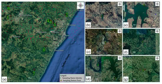
Figure 1.
Locality map for sampling stations: (a) all eight sampling stations, (b) Henley Dam, (c) Hazelmere Dam, (d) Inanda Dam, (e) Midmar Dam, (f) Umzinto Dam, and (g) Nungwane Dam. The underlying map used for the production of the locality map was downloaded from Google Earth and station coordinates are from UWB as presented in Table 2. Notes: Sampling Stations identity (1) Henley Dam DHL003, (2) Hazelmere Dam DHM003, (3) Inanda Dam 0.3 km DIN003, (4) Inanda Dam 7.5 km DIN013, (5) Inanda Dam 14.0 km DIN017, (6) Midmar Dam DMM003, (7) Umzinto Dam DMZ009, and (8) Nungwane Dam DNW003.
At least one or more stations were considered for each of the four drainage basins applicable to the study. Testing the model with data from these four river catchments supports the objective of establishing a water quality index (WQI) applicable to the greater part of the country, if not the whole of South Africa. Over and above the availability of data from UWB, the economic significance of KwaZulu-Natal Province [15,16], the distinctiveness of its inter-basin arrangements, the scope of the transfer schemes involved and extensive water demand [17,18,19]; all these, uniquely encouraged the choice of the study area, which falls under Pongola-Mtamvuna water management area (WMA) [20,21]. The project data was adequate to examine the model and complement the objective of developing a nationally acceptable proxy water quality index.
2.1.1. Umgeni River Catchment
Umgeni River catchment is a sub-humid drainage basin located along the Indian Ocean coastline in KwaZulu-Natal Province in the Republic of South Africa [16,22,23]. Umgeni River catchment has surface area nearing 4432 km2, with Umgeni River being the major water channel of the drainage basin [13,15,21,24]. The 232-km long river originates from the Drakensberg mountains and flows eastwards towards the Indian Ocean with four main cardinal tributaries namely Lions, Karkloof, Impolweni and Umsunduzi Rivers [21,23]. Lions River is the most contributing tributary on the upstream of Midmar Dam and it serves as the transfer channel conveying water resources from the adjacent Mooi River Catchment [13]. The basin land cover is characterized as heterogeneous mostly consisting of urban areas, natural forest, commercial sugarcane plantations, small-scale to commercial agricultural farms and the Port City of Durban [13,15,16,22]. Notably, Umgeni River supports the livelihood of informal settlers residing along the river course. They rely on the river for various household activities, irrigation and livestock production [25]. The rainfall pattern of Umgeni basin is seasonal, with rains concentrated in the summer months (October to March). The amount of precipitation is highly variable, increasing from the western side to the eastern part of the river catchment. The highest rainfall occurs in coastal areas with a range of 1000 mm/yr to 1500 mm/yr [15,23]. The inland parts of Umgeni basin generally receive rainfall ranging from 800 mm/yr to 1000 mm/yr [15,22,26]. The average annual temperature ranges from 12 °C to 22 °C; leading to evaporation rates between 1567 mm/yr and 1737 mm/yr [13]. Four major dams are used to regulate and preserve the water resources in Umgeni drainage region and these are, Midmar, Albert Falls, Nagle and Inanda [13,18]. Midmar Dam supplies Pietermaritzburg and some portions of Durban, whereas Albert Falls, Nagle and Inanda Dams cater for the greater part of Durban Metropolitan [21,22,23]. In addition to the four major dams, there is Henley Dam situated south of Midmar Dam along Msunduzi River, a tributary of Umgeni River. Apart from that, there are about 300 farm dams utilized for irrigating nearly 185 km2 of commercial farms in Umgeni catchment area [22,27].
2.1.2. Umdloti River Catchment
Umdloti catchment is situated north-east of Umgeni basin, adjacent to Nagle and Inanda Dams. The catchment has an estimated area of 597 km2 with Umdloti River as the main watercourse of the basin [28]. The river source is found in the Noodberg area and stretches for nearly 88 km, flowing eastwards towards the Indian Ocean. The river estuary is approximately 25 km north-east of Durban Central [24,29]. A considerable portion of the catchment is utilized for commercial farming, dominated by sugarcane and banana plantations with minimal of vegetable and citrus farming. Apart from these, other establishments include residential, Verulam Town, game reserves, Hazelmere Dam and Hazelmere wastewater treatment plant [29]. Similar to Umgeni basin, the catchment experiences summer rainfall with mean annual precipitation ranging between 800 and 1125 mm. Temperatures varying from 9 °C in winter to 38 °C in summer [29]. Hazelmere Dam is the major water impoundment in Umdloti catchment [28]. The dam was established to service the domestic, industrial and agricultural needs of the Durban area, including the new Durban International Airport [24,27,29].
2.1.3. Nungwane River Catchment
Located south-west of Umgeni drainage region, Nungwane River catchment has a mean annual precipitation of 938 mm/yr and annual evaporation close to 1200 mm/yr. The significant impoundment in the quaternary catchment is the Nungwane Dam situated along Nungwane River, which is a tributary of Lovu River [30]. The impoundment was built in 1977 with catchment area of 58 km2 and raw from Nungwane Dam is treated at Amazimtoti water treatment plant and supply eThekwini Municipality [27,30].
2.1.4. Umzinto/uMuziwezinto River Catchment
Umzinto River catchment also known as UMuziwezinto River catchment lies further south of Nungwane Dam. According to Umgeni Water [30], the river basin receives rainfall averaging 985 mm/yr, with an evaporation rate of 1200 mm/yr. In 1983, Umzinto Dam was constructed along Umzinto/uMuziwezinto River with catchment coverage of about 52 km2 [27]. Together with EJ Smith Dam, raw water from Umzinto Dam is treated at Umzinto water treatment plant (WTP) and distributed to Ugu District Municipality [30,31]. Both dams, EJ Smith and Umzinto, supply raw water towards the operation of Umzinto WTP [30,31].
2.2. Water Quality Assessment
In order to perform multiple linear regression (MLR) analysis, two variables are necessary; thus, the independent and dependent variables. In this study, water quality index (WQI) scores were regarded as the dependent variable and the measured parameter values of the physicochemical water quality variables were considered as the independent variables. Water quality index is a simple, but yet intelligible rating score that provides the composite influence of various water quality variables in a given water body [32,33,34]. The index number is normally measured against a relative scale to explain the quality of water based on categories ranging from zero to hundred [35]. In a similar fashion, the newly established universal water quality index (UWQI) was utilized for WQI assessment and the model constitute the following:
- (a)
- Variables: thirteen predefined explanatory water quality parameters (NH3, Ca, Cl, Chl-a, EC, F, CaCO3, Mg, Mn, NO3, pH, SO4 and Turb), which are listed based on expert opinion [27]. Rand Corporation’s Delphi Technique was applied to incorporate expert opinion from a panel of thirty water specialists from government parastatals, private sector and academia. Delphi Questionnaires were circulated to the participants and were asked to consider twenty-one water quality parameters for their possible inclusion in the UWQI. The panelists were instructed to designate each variable as: “Include” and “Exclude” and further assign a relative significance rating against each variable elected as “Include.” The rating scale ranged from one to five, whereby “scale 1” denoted the uppermost significance and “scale 5” represented a comparatively low significance. In addition to the prescribed twenty-one parameters, the experts were allowed to add at most five more variables if desired. A total of twenty-one questionnaires were returned out of the thirty questionnaires circulated. The Rand Corporation’s Delphi Technique is described in detail by Horton [36], Brown, et al. [37] and Linstone and Turoff [38,39], and the method is applied in several studies which include Kumar and Alappat [40], Nagels, et al. [41] and Almeida, et al. [42].
- (b)
- Weight coefficients: weight ratings (bi) ranging from one (minimum impact) to five (maximum impact) were assigned to each parameter upon aggregating significance ratings derived from the participatory based Delphi method together with significance ratings extracted from literature. Thereafter, weightage coefficients (wi) were obtained from the following Equation (1) [27,43]:where: bi is the assigned significance rating of the ith water parameter (one being the lowest rating and five the highest rating); wi is the weighted coefficient for the ith water parameter (decimal value); and n total number of the rated water quality parameters. The coefficients are represented as decimal numbers and the sum of all coefficients is one, thereby guaranteeing that the overall index value does not exceed hundred percent (w1 + w2 + w3 + …+ wn = 1 for Equations (1)). Otherwise, aggregation of sub-indices will be compromised, and deem the index model dysfunctional. The weight coefficients are presented in Table 3.wi = bi/(b1 + b2 + … + bn)
Table 3. Universal Water Quality Index (UWQI) Input Parameters and Relevant Weightage Coefficients.
- (c)
- Sub-index rating curves and functions: Sub-indices (si) and sub-index rating curves; considering that water quality parameters are monitored in different scientific units; sub-indices are applied to convert the different units of measure into a single common non-dimensional scale [44]. This is a common practice and the conventional method involves sub-index rating curves which are later transformed into mathematical functions commonly known as sub-indices. For practical purposes, fixed key points of the rating curves were graphically established with reference to the permissible concentration limits. Straight-line graphs were used to converge the plotted points and produce a series of linear graphs, which were further converted into linear sub-index functions. Target Water Quality Ranges (TWQRs) as prescribed by DWAF [45,46,47] were consulted in the process. Due to the nature of the article, only the sub-index rating curve and mathematical function for NH3 are presented herein as Figure 2 and Equation (2).where: SIa is the sub-index for ammonia (NH3) and xa is the observed water quality reading of the respective water quality parameter.
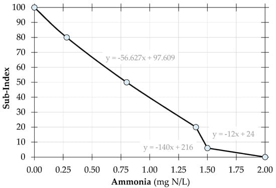 Figure 2. Sub-index rating curve for ammonia (NH3) as an example of the graphically established parameter rating curves.
 - (d)
- Aggregation formula: weighted arithmetic sum model (UWQI), which is an improved version of the weighted sum method. Scenario-based analysis was used to modify and align the model with local conditions to develop the final universal water quality index (UWQI) model as shown with Equation (3) [27]:where: UWQI is the aggregated index value ranging from zero to hundred, with zero representing water of poor quality and hundred denoting water of the highest quality; si is the sub-index value of the ith water quality parameter obtained from the sub-index linear functions and the values range from zero to hundred, similar to WQI values; wi is the weight coefficient value for the ith parameter represented as a decimal number and the sum of all coefficients is one, (w1 + w2 + w3 + … + wn = 1); n is the total number of sub-indices and in this case n = 13. WQI scores are presented as numerical value ranging from 0 to 100, where zero denotes poor water quality and hundred signifies excellent water quality.
2.3. Surrogate Water Quality Index (WQI)
For this particular model, water quality parameters were defined using a two-stage screening process as follows, (i) Delphi method conducted for the universal water quality index (UWQI), where twenty-one parameters were deduced to thirteen variables, then (ii) further reduced the parameters to four proxy variables using statistical assessment. During this procedure, principal component analysis (PCA) was used for pattern recognition and explaining the structure of the underlying dataset [48,49]. It aided in identifying intercorrelated parameters and provided important statistical information on the most significant parameters that can be used as proxy variables. Further to this, hierarchical cluster analysis (HCA) was performed to provide instinctive similarity relationships that exist among water quality parameters and in the process, HCA yielded a dendrogram (tree diagram) that illustrated the cluster arrangement and parameter proximity to one another [50,51].
Thereafter, multivariate regression analysis was adopted to estimate the relationship between WQI (dependent variable) and independent variables (predictors/covariates) which are the final four proxy parameters. The resulting regression equation and coefficients represent the surrogate WQI model. Figure 3 illustrates the model architecture applied in developing the surrogate WQI.
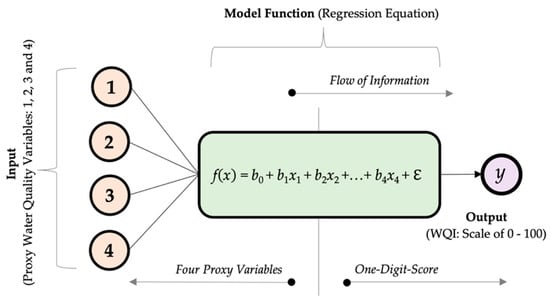
Figure 3.
Model architecture applied in the development of the surrogate water quality index model using four proxy water quality variables. A model outline displaying the structure of the surrogate WQI with four proxy water quality input variables x1, x2, x3 and x4; their corresponding coefficients b1 to b4, intercept term b0, error term for the regression model symbolized as ℇ, and the regression model function f(x) = b0 + b1x1 + b2x2 +…+ b4x4 + ℇ as the surrogate WQI.
The advantage of this method is that optimum selected parameters can still describe water quality in the absence of the entire dataset [50,52]. It provides an important quick-guide identical to the outcome of high-fidelity model and conforms to the requirements of the study. All the statistical computations were performed using IBM SPSS Statistics Version 24 for MacOS [53].
2.4. Water Classification
In the interest of simplifying the interpretation of water quality index (WQI) values, mostly to accommodate non-technical individuals, an index categorization schema was established. The classification mechanism is based on an increasing scale index and the advantage of this system is that it is identical to a normal percentage hierarchy [43], therefore the public can easily relate to its function and interpretation. Both models applicable to this study yields WQI values between zero and hundred. Accordingly, the WQI scores are categorized using classes ranging from one to five; with “Class 1” representing water of the highest degree of purity with a possible maximum score of hundred and vice versa, “Class 5” denotes water quality of the poorest degree with index scores nearing or equal to zero. In order to close gaps identified in some of the existing classification scales [44], appropriate mathematical functions with logical linguistic descriptors which includes but not limited to, “greater than,” “less than,” “equal to,” are used to appraise WQI scores and respectively assigned them to the corresponding category.
3. Results and Discussion
3.1. Rationale for Developing Surrogate Water Quality Index (Multiple Linear Regression Model)
Consider a range of data comprising of n statistical units (observations) of the response variable y (dependent variable) and p-vector of regressors x (independent explanatory variable); then, their mathematical relationship is designated as a linear regression model in the form [54,55]:
y = b0 + b1x1 + b2x2 +…+ bpxp + ℇ
The observations are assumed to be the result of random deviations from an underlying relationship between the dependent variable (y) and the independent variable (x). With regards to observed data, the linear function is defined as [54,55]:
where i = 1, 2, …, n and variables ℇi symbolize unobservable regression model errors, which are presumed to be independent and identically distributed random variables; with a distribution function F and density f. Of which, the density is unknown and expected to be symmetric at zero (0). The corresponding coefficients b1 to bp and intercept term b0, are unknown values calculated based on the dependent variable y = (y1, y2, …, yn) and independent variable x = (xi1, xi2, …, xip). Besides the orthodox least-squares method, various statistical estimators of model coefficient (b) exist and they are documented in literature. Some of the methods are distributionally robust (less sensitive to deviations from the assumed distribution factors), whilst others are resistant to the leverage points in the design matrix and have a high breakdown point [54]. Following the above rationale, linear regression was considered in the development of the proxy water quality index model and the results are documented in the following subsections.
yi = b0 + b1xi1 + b2xi2 +…+ bpxip + ℇi
3.2. Significant Parameters Applicable to the Surrogate Water Quality Index (WQI)
A combination of two methods has been adopted in the selection of the most suitable explanatory variables for the suggested proxy model. The methods include, (1) the Rand Corporation’s Delphi Technique (Delphi method) and, (2) multivariate statistical analysis. The Delphi method has been employed to abridge the list of parameters from twenty-one to thirteen variables which are applicable to the universal water quality index (UWQI). Furthermore, statistical analysis assisted in reducing the parameters to four proxy variables applicable to the surrogate WQI. Principal component analysis (PCA) have been performed for pattern recognition and outlining the framework of the project data. Whereas hierarchical cluster analysis (HCA) helped to establish the degree of similarity among water quality parameters. Accordingly, electrical conductivity, chlorophyll-a, pH turbidity are the final four proxy parameters considered for the surrogate WQI. Figure 4 illustrates the two-stage screening process established to select significant water quality parameters.
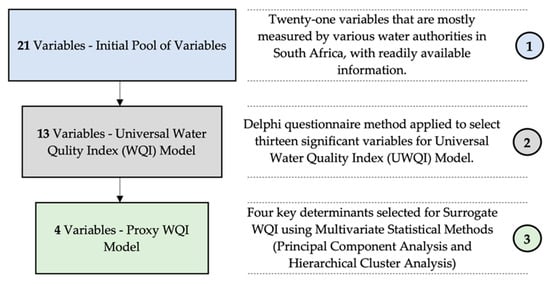
Figure 4.
Flow diagram illustrating the two-stage screening process employed for selecting the significant water quality parameters. Source: Umgeni water quality data. Notes: statistical analysis was performed using water quality dataset from Umgeni Water Board monitored from January 2012 to July 2018.
Additional information relating to the selection of these input variables is discussed and presented in the succeeding sections.
3.3. Multivariate Statistical Analysis
3.3.1. Principal Component Analysis (PCA)
Considering that water quality is generally described using multiple physicochemical and biological variables; principal component analysis (PCA) can ideally transform complex multivariate datasets to a minimal and manageable number of factors without loss of information [56,57]. More importantly, PCA preserves the structure and pattern of the original dataset to the maximum extent possible [11,12]. PCA is an accurate and extensive method for parameter reduction; which is significant and can drastically lower assessment cost, time and effort, thereby promoting routine monitoring.
The rationale behind PCA is centered on decreasing dimensions of multivariate dataset through summarizing information dispersed in several dimensions into reduced number of dimensions that are not correlated [11,58,59]. The technique eliminates collinearity amongst explanatory variables, discard redundant or extremely correlated variables and develop new uncorrelated variables known as principal components (PCs) [60,61]. The application of statistical techniques in the development of water quality indices (WQIs) lessens biasness and makes them more objective in nature [11].
The first step in performing PCA involves delineating the number of PCs that can adequately explain the structure and pattern of a given dataset. This process is accomplished by the use of (a) scree-plot, (b) real data eigenvalues, and (c) randomly generated eigenvalues. It should be noted that, although it is common practice to disregard low-variance PCs, sometimes they can be useful in their own right; for instance, they can assist in identifying outliers and enhance quality control [56]. Ideally for PCA to draw purposeful and reliable conclusions, the standard advice is to retain factors characterized by the following [62]:
- (a)
- Related eigenvalues that are greater than one (>1.0);
- (b)
- Initial eigenvalues percentage of variance of greater than ten percent (>10%); and
- (c)
- Cumulative percentage of variance of greater than sixty percent (>60%).
However, these are just suggestive figures and should be regarded as indicative of the ideal situation. Notably, different opinions exist in literature, especially on the cumulative percentage of variance contribution. Tripathi and Singal [62] suggest a minimum of 60%, whereas Jolliffe [56] and Gradilla-Hernández, et al. [63] propose a range between 70% and 90% with an acknowledgment that the value can be higher or lower depending on the context of the dataset.
Figure 5 represents a scree-plot developed using real data eigenvalues assisted in identifying the number of principal components to be extracted. Corresponding to the scree-plot sagging point; principal components with eigenvalues greater than one (latent-root-one) were considered significant to explain the underlying structure of the dataset [12,62,64,65,66,67]. Complementary, Parallels Analysis Engine (PAE) aided in confirming the number of factors retained. Using research data, PAE computed eigenvalues from randomly generated correlation matrices, which were used to intercept the cut-off point on the scree-plot diagram. Both PCA and PAE eigenvalues were presented graphically as two different plots, and their intercept point established the number of factors retained during multivariate statistical analysis [64,68]. All the principal components above the PAE graph were considered; in this case, the first five factors were deemed statistically important.
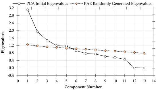
Figure 5.
Determination of Principal Components (PCs) to be extracted using eigenvalues from Principal Component Analysis (PCA) and randomly generated eigenvalues from Parallel Analysis Engine (PAE). Source: PCA results from IBM SPSS Statistics [53] and Parallel Analysis Engine [68]. Notes: randomly generated eigenvalues were established using PEA, whereas PCA eigenvalues were established using dataset from Umgeni Water Board.
In order to obtain meaningful and more accurate results, the dataset subjected to principal component analysis should have a minimum of 150–300 test cases [11,12,62,69]. Accordingly, the current study used 638 test cases monitored from eight sampling stations observed weekly for a period of six and half years (refer to Table 1). The case study surpasses the recommended threshold, thus satisfying the stated criterion.
The study performed Kaiser-Meyer-Olkin (KMO) and Bartlett’s test of sphericity to authenticate the suitability of the dataset to effectively handle principal component analysis (PCA) and factor analysis (FA). KMO is the measure of sampling adequacy that signifies the degree of variance caused by underlying principal components (PCs) [65]. Generally, KMO values below 0.5 are undesirable, whereas values ranging from 0.5 to 0.7 are considered sufficient and higher values (above 0.7) are exceptionally good [11,59,67,70]. The current study achieved KMO value of 0.510, which is satisfactory.
Bartlett’s test examines the possibility of the correlation matrix being an identity matrix. If such a possibility exists; Bartlett’s test of sphericity assumes that all variables are unrelated and dimensionality reduction is not feasible, thus making PCA and FA inapplicable. Bartlett’s test scores less than 0.050 are favorable and suggest that significant relationships exist among variables [11]. In the current case, Bartlett’s significance level is 0.000, thus confirming the appropriateness to perform principal component analysis and factor analysis.
Correlation matrix assisted in evaluating inter-relationships between the thirteen water quality variables shortlisted for statistical analysis. Similar to Nnorom, et al. [59], Patil, et al. [67], Ustaoğlu, et al. [70], and Wang [71], the classification adopted is defined as follows: (a) r < 0.3, considered of no relevance; (b) 0.3 ≤ r < 0.5, less relevance; (c) 0.5 ≤ r < 0.8, median relevance; and (d) r ≥ 0.8, high relevance. Considering such groupings, the analysis indicates that Mg is highly related to Ca and CaCO3. Though with less relevance, the results suggest that NH3 is correlated with EC and NO3.
As a common practice, rotation (Oblimin with Kaiser Normalization) was executed to ensure that variables with higher loading values are not considered on the same factor. Rotation transforms the factorial axes into a structure where each of the retained factors are preferably loaded with only one variable. Furthermore, especially where few principal components (PCs) exist, rotation restricts variables to overlay factor loadings on more than one principal component (PC) [62]. Post rotation, the leading parameters with the highest loadings are grouped as intermediate composites and assigned weights. The weights are then aggregated and their compound effect is proportional to the percentage of variance explained by a particular component [62].
Considering that water quality parameters have different units, standardization (z-scores) harmonized the dataset to a common scale with zero mean and unit standard deviation [11,12,56,60,61,72].
Table 4 presents the correlation matrix, KMO and Bartlett’s test results, whereas the five extracted principal components (PCs) are presented in Table 5.
Table 4.
Correlation Matrix, Kaiser-Meyer-Olkin (KMO) and Bartlett’s Test Results for Thirteen Physico-Chemical Variables Shortlisted for Multivariate Statistical Analysis.
Table 5.
Principal Component Analysis Vector of Coefficients for First Five Principal Components (PCs) with Eigenvalues Greater Than One (>1.0) for Umgeni Water Quality Data.
PCA helped in reducing the dimensionality of the dataset and summarized the variables to five important components. The first five PCs retained accounted for about 69% of the total variance with eigenvalues greater than one (>1.0). For ease reference and factor interpretation, factor loadings are classified as “weak,” “moderate,” and “strong” corresponding to absolute loading values of 0.3 to 0.5, 0.5 to 0.8 and >0.8 respectively [59,67,70]. Having strong positive loadings of 0.979, 0.972 and 0.979 for Ca, Mg and CaCO3 respectively, the first component (PC 1) accounts for almost 24% of the total variance with eigenvalue of 3.118. The second PC features moderate loadings of −0.681, 0.624 and 0.522 corresponding to NH3, NO3 and EC with eigenvalue of 1.948 and variance of nearly 15%. Moderate factor loadings of SO4 (−0.654), Mn (0.624), and Turb (0.522) dominate the third component (PC 3) which represents about 11% of the original variability with eigenvalue of 1.482. Signifying just about 9% variance and eigenvalue of 1.195, the fourth factor (PC 4) contains fluoride as the most significant variable with a strong positive factor loading of 0.763. Lastly, the fifth component (PC 5) accounts for approximately 9% of the total variance with eigenvalue of 1.171. This component is dominated by two parameters, thus pH and Cl, with moderate factor loadings of 0.610 and −0.629 respectively.
Principal component analysis (PCA) is the most used tool in exploratory data analysis and provides a real interpretation of multi-constituent measurements which enables a better understanding of water quality composition [11,56,63,67]. PCA is a common primary method used for pattern recognition and the technique is regarded as the simplest of the true eigenvector-based multivariate analyses. One of the most effective and informative graphical illustrations of multivariate analysis is through the use of biplots. They optimally represent relationships between variables and principal components. Biplots suggest groups of highly correlated variables using an approximation of the original multidimensional space [63,68]. Biplots are illustrated in either two or three-dimensional subspace. On that basis, the statistical results of the current study are further explained using 2D and 3D biplots in Figure 6 and Figure 7, respectively.
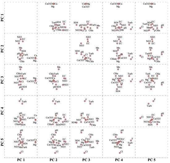
Figure 6.
2D biplot showing the relationship between highly correlated variables and the first five retained principal components (PCs). The five principal components (PCs) are denoted as PC 1, PC 2, PC 3, PC 4 and PC 5. Variables are ammonia (NH3), calcium (Ca), chloride (Cl), chlorophyll-a (Chl-a), electrical conductivity (EC), fluoride (F), hardness (CaCO3), magnesium (Mg), manganese (Mn), nitrate (NO3), pondus Hydrogenium (pH), sulphate (SO4) and turbidity (Turb). Source: PCA results from IBM SPSS Statistics [53].
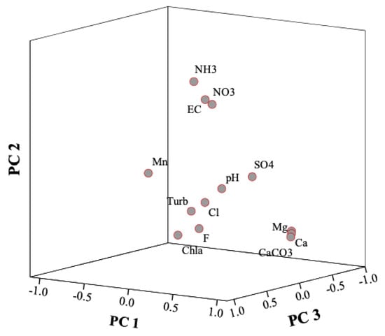
Figure 7.
3D biplot illustrating the relationship between highly correlated variables and the first three principal components. Source: PCA results from IBM SPSS Statistics [53].
3.3.2. Hierarchical Cluster Analysis (HCA)
Hierarchical cluster analysis (HCA) essentially outlined the hierarchical relationships between variables and assisted in arranging thirteen variables into corresponding clusters. Various hierarchical clustering methods exist, but in this study, centroid based clustering algorithms and Ward’s hierarchical clustering methods were examined. Eventually, Ward’s technique was preferred amongst the two methods. Ward’s procedure generates approximately identical grouped clusters, unlike the other methods, where groupings are not equally proportional [63].
Cluster analysis uses distance matrix and the model intervals were calculated using squared Euclidean distance technique [63,73]. The method is regarded as the best option and most appropriate measure of distance in the physical world. Since variables are measured in different units, standardization was performed to transform the observed measurements into a common scale. The tree diagram in Figure 8 represents the hierarchical clustering dendrogram for the thirteen explanatory variables considered in the analysis.
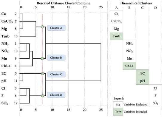
Figure 8.
Hierarchical clustering dendrogram model for water quality variables using Ward’s Linkage and Euclidean Distance method (Hierarchical Cluster Analysis). Source: HCA results from IBM SPSS Statistics [53].
As expected, extremely correlated variables are clustered together. For example, variables from principal component one are all grouped together under ‘Hierarchical Cluster A.’ Likewise, variables in principal component two are included in the second group of the hierarchical cluster dendrogram. The four clusters assisted in selecting the final four proxy variables incorporated in the surrogate index. At this stage, two sets of variables were considered as input parameters for the surrogate WQI. The sets are grouped as:
- (a)
- Turb, Chl-a, EC and SO4 —proxy WQI(a); and
- (b)
- Turb, Chl-a, EC and pH—proxy WQI(b).
Multivariate statistical analyses are highly objective in nature, and their application in WQI development makes the process unbiased [11,12,62,67]. However, the process does not incorporate local conditions and or expert opinion. Nevertheless, this study integrated professional judgment through the decision to include pH as input parameter, even though the variable is extremely correlated to EC; the individual importance of pH could not be neglected, hence the need to evaluate the performance of proxy WQI(b).
3.3.3. Multiple Linear Regression (MLR)
As previously stated, multiple linear regression (MLR) analysis was performed to establish regression coefficients of the two preliminary surrogate index models. MLR is a statistical procedure that predicts the values of the dependent (response) variable from a multiple of independent (exploratory) variables. More precisely, MLR analysis enables the estimation of y-value for specified values of x1, x2, …, xk [55,72]. Durbin-Watson (DW) method was employed considering that water quality data is time-series; each case or test is time-based. DW technique uses the “line of best fit” technique to establish the linear regression equation. All the significant proxy variables were subjected to MLR to determine optimal linear fitting and generate the best regression coefficients used to establish an empirical mathematical equation applicable in evaluating the purity of surface water. Following the results of the multiple linear regression, the subsequent mathematical coefficients in Table 6 have been suggested for the two preliminary proxy models.
Table 6.
Multiple Linear Regression (MLR) Coefficients for Two Preliminary Surrogate Models, Proxy WQI(a) and Proxy WQI(b).
Once the multiple regression equation is developed, the appropriateness and predictive ability of the model can be examined using values of known scenarios. Therefore, with the aim of validating the selection of four key proxy variables, the two preliminary surrogate water quality indices were subjected to a scenario-based analysis. The outcome of the procedure is documented in the following subsection.
3.4. Scenario-Based Model Validation Analysis
Scenario-based analysis helps identify potential data-processing gaps, which in turn enlighten on the necessary precautions imperative to minimize the impact, or perhaps eliminate the problem. To determine such, ideal sets of predictive variables have been established under a variety of scenarios to calculate specific water quality variables. Considering increments of five scores, nine probable scenarios have been examined to demonstrate the model’s ability to predict scores of all ranges, from class one (excellent) to class five (worse). The nine forecasts are founded on three-level-grading, which comprise of (i) worst-case scenario, 0 ≤ Index ≤ 10; (ii) base-case scenario, 45 ≤ Index ≤ 55; and lastly (iii) best-case scenario, 90 ≤ Index ≤ 100. Purposefully, the groupings provided a complete change of circumstances with each scenario, thereby widening the range of analysis and include a considerable array of possibilities. With reference to permissible concentration limits and developed linear sub-index functions (see Figure 2 and Equation (2)); definite assumptions about all nine cases have been carefully considered. Accordingly, parameter values corresponding to each scenario have been established and applied to perform the analysis [27]. Following this procedure, the two proxy WQIs have been examined to delineate their proficiency and ability to analyze water quality data. The nine scenarios and parameter values used herein, are identical to those applied for UWQI, and the scenario-based analysis results for the surrogate WQIs are included as Table 7 and Figure 9.
Table 7.
Comparison of the Developed Proxy Water Quality Indices (a) and (b) Using Scenario-Based Analysis to Establish the Functionality and Predictive Capacity of the Models.
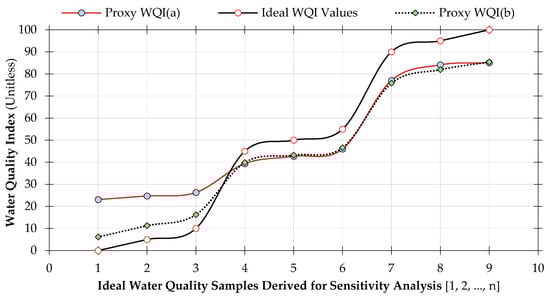
Figure 9.
Plot diagram showing the results of the scenario-based analysis of the developed proxy water quality indices (a) and (b) against ideal water quality values derived from nine probable scenarios. The nine cases presented herein, are similar to those applied for UWQI and they are represented as samples 1, 2, …, n, which corresponds respectively to water quality (WQI) values of 0, 5, 10 (worst-cases); 45, 50, 55 (base cases); and 90, 95, 100 (best cases).
Both proxy WQIs have comparable predictive patterns, which are consistent with the ideal graph. Furthermore, both models have corresponding water quality scores for base-case and best-case scenarios. Except for the worst-case scenario, the two indices have different results, with proxy WQI(b) being much closer to the ideal graph than proxy WQI(a). Ultimately, the analysis proved that surrogate WQI(a) struggles to evaluate water quality samples with higher parameter concentrations. Against this background, proxy WQI(b) is then considered as the most appropriate surrogate index developed for this study. The model, as represented by Equation (6), functions with four input variables, namely turbidity, chlorophyll-a, electrical conductivity and pondus Hydrogenium. This aligns with the objective of the study, which involves establishing four proxy determinants for the surrogate WQI and assign relative coefficients for the model:
where WQI is the calculated index value ranging from zero to hundred, with zero representing water of poor quality and hundred denoting water of the highest quality; Chl-a is the observed chlorophyll-a concentration in micrograms per litre (µg/L); pH is the observed pondus Hydrogenium levels which are unitless; Turb is the observed turbidity concentration measured in Nephelometric Turbidity Units (NTU); and EC is the electrical conductivity concentration in micro Siemens per meter (µS/m).
WQI = 85.273 − 0.042Chl-a + 0.224pH − 0.090Turb − 0.151EC
Umgeni water quality data have been examined to further demonstrate the applicability of the proposed surrogate index, and the results are presented in the following plot diagram (Figure 10).
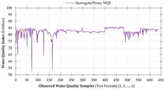
Figure 10.
Water quality index results calculated using the proposed surrogate water quality index for Umgeni water quality data for a period of six and half years from January 2012 to July 2018. The Umgeni Dataset is from eight sampling stations which fall under four different catchment areas namely, Umgeni River catchment (Henley, Inanda and Midmar Dams); Umdloti River catchment (Hazelmere Dam); Nungwane River catchment (Nungwane Dam); and lastly Umzinto/uMuziwezinto River catchment (Umzinto Dam).
In view of the curtailed 638 water quality samples, spatial and temporal changes in water quality for Umgeni Water Board are evident over the past six and half years, with a much varying sequence comprising of index scores as high as 85.8 (class two), an average of 82.5 (class two) and the lowest score of 52.9 (class three).
Of great importance, the surrogate WQI model responded remarkably to the variation of water quality parameter values, with the index output graph confirming to the fluctuations. This advocates the readiness of the proxy WQI to interpret water quality data and provide a simple non-dimensional score that is justifiable and in a repeatable manner. Such success fulfills the objective of the study and more importantly presents a “yardstick” that can be applied in most, if not all the distinct watersheds in South Africa. This accomplishment is a critical milestone, not only for the authors but to most of the stakeholders directly or indirectly involved in water quality science.
Index scores from water quality index model are classified using a common index categorization schema. The focus is on maintaining a standardized unit and compare results of the same group. The index categorization schema developed for the study is described in the following section.
3.5. Index Categorisation Schema
Water quality index (WQI) classification approach integrates WQI results into a much simpler, but yet decisive expression that can describe the spatial and temporal changes in water quality. Water categorization has brought more clarity and understanding in the interpretation of water quality index scores, making it more favorable to non-technical individuals and water management officials.
Accordingly, an increasing scale index with values ranging from zero to hundred (0 to 100) with categorization classes ranging from Class 1 to Class 5 has been adopted for the classification of the water quality index scores. Class 1 water quality with a possible maximum index score of hundred (100) represents water quality of the highest degree, whereas Class 5 water quality with an index score close or equal to zero (0) denotes water quality of the poorest degree [27].
Table 8 indicates the index score classification for the water quality index proposed for South African watersheds and eventually satisfying the objective of producing a water classification grading and water categorization schema suitable for assessing South African river catchments.
Table 8.
Index Score Classification for the Surrogate Water Quality Index for South African River Catchments.
Similar to the methods used by Abrahão, et al. [74], Rabee, et al. [75], Rubio-Arias, et al. [76] and Sutadian, et al. [77], appropriate mathematical functions with logical linguistic descriptors such as less than, equal to and greater than have been assigned to each categorization class. By so doing, the categorization schema can accommodate all possible index scores regardless of the decimal value. This method ultimately assists in developing more flexible and precise water quality models. More importantly, the established categorization schema aids in closing gaps identified in literature [27,44], and present a progressive approach that will contribute significantly towards water quality indices development. Such an academic contribution reflects on the efficiency of the model and attributes to the success of the current study.
4. Conclusions
A scientifically balanced surrogate water quality index (WQI) has been suggested. Multivariate statistical method has been effectively adopted and employed for selecting four proxy parameters and establishing their relative coefficients. Two models were developed, each with four indicators; in fact, the first three variables are similar except the forth parameter of each model. The identical variables are chlorophyll-a (Chl-a), electrical conductivity (EC) and turbidity (Turb). Proxy WQI(a) has sulphate (SO4) as the fourth parameter, whereas proxy WQI(b) uses pondus Hydrogenium (pH) instead. Both models are technically sensible, with the latter model being considered as the most applicable proxy index. The four parameters retained in the proposed proxy model can be easily measured, even using remote sensors; which would drastically reduce time, effort and cost of evaluating water quality across South African river catchments.
The proxy WQI is not intended at substituting comprehensive water quality evaluations instead, it is designed to deliver a quick guide of water resources status, which should assist water quality experts, policymakers and the public by communicating water quality data in a more consistent and on-going manner. Developing the surrogate WQI is an attempt to provide an alternative index, better functional with minimum variables, especially in the absence of a full-dataset applicable to high-fidelity model referred to as universal water quality index (UWQI). Though with a slight prediction disparity, the proxy WQI can systematically replicate the prediction capabilities of the UWQI. The surrogate WQI developed under this study is regarded as an achievement and considered successful enough to fulfill the objective of the research. The objective is defined as developing a surrogate water quality index model that can operate with four key determinants as a proxy to the unbridged UWQI.
Author Contributions
Conceptualization, T.D.B. and M.K.; methodology, T.D.B.; software, T.D.B.; validation, T.D.B. and M.K.; formal analysis, T.D.B.; investigation, T.D.B.; resources, T.D.B. and M.K.; data curation, T.D.B.; writing—original draft preparation, T.D.B.; writing—review and editing, T.D.B. and M.K.; visualization, T.D.B.; supervision, M.K.; project administration, T.D.B.; funding acquisition, T.D.B. and M.K. All authors have read and agreed to the published version of the manuscript.
Funding
This research was funded by ZAKUMI Consulting Engineers (Pty) Ltd., grant number ST2017/BANDA/PhD-Eng/UKZN and the research was supported by the University of KwaZulu-Natal.
Acknowledgments
Our utmost gratitude is extended to the staff members of the Research Office of the University of KwaZulu-Natal for supporting this research publication.
Conflicts of Interest
The authors declare no conflict of interest. The funders had no role in the preparation of this paper; in the collection, analyses, or interpretation of data; in the writing of the manuscript, or in the decision to publish the paper.
References
- Pegram, G.; Görgens, A. A Guide to Non-Point Source Assessment: To Support Water Quality Management of Surface Water Resources in South Africa (WRC Project No. 696/2/01); Water Research Commission: Cape Town, South Africa, 2001; p. 127. [Google Scholar]
- Ochieng, G.M. Hydrological and Water Quality Modelling of the Upper Vaal Water Management Areas Using a Stochastic Mechanistic Approach. DTech Thesis, Tshwane University of Technology, Pretoria, South Africa, 2007. [Google Scholar]
- Razavi, S.; Tolson, B.A.; Burn, D.H. Review of surrogate modeling in water resources. Water Resour. Res. 2012, 48. [Google Scholar] [CrossRef]
- Asher, M.J.; Croke, B.F.W.; Jakeman, A.J.; Peeters, L.J.M. A review of surrogate models and their application to groundwater modeling. Water Resour. Res. 2015, 51, 5957–5973. [Google Scholar] [CrossRef]
- Bhosekar, A.; Ierapetritou, M. Advances in surrogate based modeling, feasibility analysis, and optimization: A review. Comput. Chem. Eng. 2018, 108, 250–267. [Google Scholar] [CrossRef]
- Schultz Martin, T.; Small Mitchell, J.; Farrow, R.S.; Fischbeck Paul, S. State Water pollution control policy insights from a reduced-form model. J. Water Resour. Plan. Manag. 2004, 130, 150–159. [Google Scholar] [CrossRef]
- Shamir, U.; Salomons, E. Optimal real-time operation of urban water distribution systems using reduced models. J. Water Resour. Plan. Manag. 2008, 134, 181–185. [Google Scholar] [CrossRef]
- Castelletti, A.; Pianosi, F.; Soncini-Sessa, R.; Antenucci, J.P. A multiobjective response surface approach for improved water quality planning in lakes and reservoirs. Water Resour. Res. 2010, 46. [Google Scholar] [CrossRef]
- Preis, A.; Whittle Andrew, J.; Ostfeld, A.; Perelman, L. Efficient hydraulic state estimation technique using reduced models of urban water networks. J. Water Resour. Plan. Manag. 2011, 137, 343–351. [Google Scholar] [CrossRef]
- Sreekanth, J.; Datta, B. Coupled simulation-optimization model for coastal aquifer management using genetic programming-based ensemble surrogate models and multiple-realization optimization. Water Resour. Res. 2011, 47. [Google Scholar] [CrossRef]
- Tripathi, M.; Singal, S.K. Use of Principal Component Analysis for parameter selection for development of a novel Water Quality Index: A case study of river Ganga India. Ecol. Indic. 2019, 96, 430–436. [Google Scholar] [CrossRef]
- Jahin, H.S.; Abuzaid, A.S.; Abdellatif, A.D. Using multivariate analysis to develop irrigation water quality index for surface water in Kafr El-Sheikh Governorate, Egypt. Environ. Technol. Innov. 2020, 17, 100532–100543. [Google Scholar] [CrossRef]
- Namugize, J.N.; Jewitt, G.; Graham, M. Effects of land use and land cover changes on water quality in the uMngeni river catchment, South Africa. Phys. Chem. Earth Parts A/B/C 2018, 105, 247–264. [Google Scholar] [CrossRef]
- Schullehner, J.; Jensen, N.L.; Thygesen, M.; Hansen, B.; Sigsgaard, T. Drinking water nitrate estimation at household-level in Danish population-based long-term epidemiologic studies. J. Geochem. Explor. 2017, 183, 178–186. [Google Scholar] [CrossRef]
- Shoko, C. The effect of spatial resolution in remote sensing estimates of total evaporation in the uMgeni catchment. Master's Thesis, University of KwaZulu-Natal, Pietermaritzburg, South Africa, 2014. [Google Scholar]
- Hughes, C.; de Winnaar, G.; Schulze, R.; Mander, M.; Jewitt, G. Mapping of water-related ecosystem services in the uMngeni catchment using a daily time-step hydrological model for prioritisation of ecological infrastructure investment–Part 1: Context and modelling approach. Water SA 2018, 44, 577–589. [Google Scholar] [CrossRef]
- Umgeni Water. Umgeni Water Annual Report 2017/2018 Financial Year; Umgeni Water: Pietermaritzburg, South Africa, 2018; p. 208. [Google Scholar]
- Umgeni Water. Infrastructure Master Plan 2019/2020–2049/2050, Volume 2: Mgeni System; Umgeni Water: Pietermaritzburg, South Africa, 2019; p. 185. [Google Scholar]
- Umgeni Water. Infrastructure Master Plan 2019/2020–2049/2050, Volume 3: UMkhomazi System; Umgeni Water: Pietermaritzburg, South Africa, 2019; p. 35. [Google Scholar]
- Republic of South Africa. Proposed new nine (9) water management areas of South Africa. In Government Gazette No. 35517, Notice No. 547; Department of Water Affairs and Foresty: Pretoria, South Africa, 2012; Volume 565, p. 72. [Google Scholar]
- Chiluwe, Q.W. Assessing the Role of Property Rights in Managing Water Demand: The Case of uMgeni River Catchment; Monash South Africa: Johannesburg, South Africa, 2014. [Google Scholar]
- Warburton, M.L.; Schulze, R.E.; Jewitt, G.P.W. Hydrological impacts of land use change in three diverse South African catchments. J. Hydrol. 2012, 414, 118–135. [Google Scholar] [CrossRef]
- Rangeti, I. Determinants of key drivers for potable water treatment cost in uMngeni Basin. Master's Thesis, Durban University of Technology, Durban, South Africa, 2015. [Google Scholar]
- Olaniran, A.O.; Naicker, K.; Pillay, B. Assessment of physico-chemical qualities and heavy metal concentrations of Umgeni and Umdloti Rivers in Durban, South Africa. Environ. Monit. Assess. 2014, 186, 2629–2639. [Google Scholar] [CrossRef] [PubMed]
- Gakuba, E.; Moodley, B.; Ndungu, P.; Birungi, G. Occurrence and significance of polychlorinated biphenyls in water, sediment pore water and surface sediments of Umgeni River, KwaZulu-Natal, South Africa. Environ. Monit. Assess. 2015, 187, 568. [Google Scholar] [CrossRef]
- Namugize, J.N.; Jewitt, G.P.W. Sensitivity analysis for water quality monitoring frequency in the application of a water quality index for the uMngeni River and its tributaries, KwaZulu-Natal, South Africa. Water SA 2018, 44, 516–527. [Google Scholar] [CrossRef]
- Banda, T.D.; Kumarasamy, M. Development of a Universal Water Quality Index (UWQI) for South African river catchments. Water 2020, 12, 1534. [Google Scholar] [CrossRef]
- Umgeni Water. Infrastructure Master Plan 2019/2020–2049/2050, Volume 5: North Coast System; Umgeni Water: Pietermaritzburg, South Africa, 2019; p. 116. [Google Scholar]
- Govender, S. An Investigation of the Natural and Human Induced Impacts on the Umdloti Catchment. Master's Thesis, University of KwaZulu, Natal, Durban, 2009. [Google Scholar]
- Umgeni Water. Infrastructure Master Plan 2019/2020–2049/2050, Volume 4: South Coast System; Umgeni Water: Pietermaritzburg, South Africa, 2019; p. 116. [Google Scholar]
- Mwelase, L.T. Non-revenue water: Most suitable business model for water services authorities in South Africa: Ugu District Municipality. Master's Thesis, Durban University of Technology, Durban, South Africa, 2016. [Google Scholar]
- Luzati, S.; Jaupaj, O. Assessment of Water Quality Index of Durresi-Kavaja Basin, Albania. J. Int. Environ. Appl. Sci. 2016, 11, 277–284. [Google Scholar]
- Wanda, E.M.; Mamba, B.B.; Msagati, T.A. Determination of the water quality index ratings of water in the Mpumalanga and North West provinces, South Africa. Phys. Chem. Earth 2016, 92, 70–78. [Google Scholar] [CrossRef]
- Guettaf, M.; Maoui, A.; Ihdene, Z. Assessment of water quality: A case study of the Seybouse River (North East of Algeria). Appl. Water Sci. 2017, 7, 295–307. [Google Scholar] [CrossRef]
- Paun, I.; Cruceru, L.V.; Chiriac, L.F.; Niculescu, M.; Vasile, G.G.; Marin, N.M. Water Quality Indices-methods for evaluating the quality of drinking water. In Proceedings of the 19th INCD ECOIND International Symposium—SIMI 2016, “The Environment and the Industry”, Bucharest, Romania, 13–14 October 2016; pp. 395–402. [Google Scholar]
- Horton, R.K. An Index-Number System for Rating Water Quality. J. Water Pollut. Control. Fed. 1965, 37, 300–306. [Google Scholar]
- Brown, R.M.; McClelland, N.I.; Deininger, R.A.; Tozer, R.G. A water quality index—Do we dare? Water Sew. Work. 1970, 117, 339–343. [Google Scholar]
- Linstone, H.A.; Turoff, M. The Delphi method: Techniques and applications; Addison-Wesley Reading: Reading, MA, USA, 1975; Volume 29. [Google Scholar]
- Linstone, H.A.; Turoff, M. The Delphi Method: Techniques and applications; Addison-Wesley Publishing Company, Advanced Book Program: Newark, NJ, USA, 2002; Volume 18. [Google Scholar]
- Kumar, D.; Alappat, B.J. NSF-Water Quality Index: Does It Represent the Experts’ Opinion? Pract. Period. Hazard., Toxic, Radioact. Waste Manag. 2009, 13, 75–79. [Google Scholar] [CrossRef]
- Nagels, J.; Davies-Colley, R.; Smith, D. A water quality index for contact recreation in New Zealand. Water Sci. Technol. 2001, 43, 285–292. [Google Scholar] [CrossRef] [PubMed]
- Almeida, C.; González, S.O.; Mallea, M.; González, P. A recreational water quality index using chemical, physical and microbiological parameters. Environ. Sci. Pollut. Res. 2012, 19, 3400–3411. [Google Scholar] [CrossRef] [PubMed]
- Banda, T.D. Developing an equitable raw water pricing model: The Vaal case study. Master's Thesis, Tshwane University of Technology, Pretoria, South Africa, 2015. [Google Scholar]
- Banda, T.D.; Kumarasamy, M.V. Development of Water Quality Indices (WQIs): A Review. Pol. J. Environ. Stud. 2020, 29, 2011–2021. [Google Scholar] [CrossRef]
- DWAF. South African Water Quality Guidelines: Volume 1: Domestic Water Use; Department of Water Affairs and Forestry: Pretoria, South Africa, 1996; p. 190.
- DWAF. South African Water Quality Guidelines: Volume 3: Industrial Use; Department of Water Affairs and Forestry: Pretoria, South Africa, 1996.
- DWAF. South African Water Quality Guidelines: Volume 7: Aquatic Ecosystems; Department of Water Affairs and Forestry: Pretoria, South Africa, 1996.
- Wold, S.; Esbensen, K.; Geladi, P. Principal component analysis. Chemom. Intell. Lab. Syst. 1987, 2, 37–52. [Google Scholar] [CrossRef]
- Bouza-Deaño, R.; Ternero-Rodriguez, M.; Fernández-Espinosa, A. Trend study and assessment of surface water quality in the Ebro River (Spain). J. Hydrol. 2008, 361, 227–239. [Google Scholar] [CrossRef]
- Zhao, Y.; Xia, X.H.; Yang, Z.F.; Wang, F. Assessment of water quality in Baiyangdian Lake using multivariate statistical techniques. Procedia Environ. Sci. 2012, 13, 1213–1226. [Google Scholar] [CrossRef]
- Khalil, B.; Ou, C.; Proulx-McInnis, S.; St-Hilaire, A.; Zanacic, E. Statistical assessment of the surface water quality monitoring network in Saskatchewan. Water, Air, Soil Pollut. 2014, 225, 2128. [Google Scholar] [CrossRef]
- Karamizadeh, S.; Abdullah, S.M.; Manaf, A.A.; Zamani, M.; Hooman, A. An overview of principal component analysis. J. Signal Inf. Process. 2013, 4, 173. [Google Scholar] [CrossRef]
- SPSS Inc. IBM SPSS Statistics, 24; SPSS Inc.,: Chicago IL, USA, 2016. [Google Scholar]
- Jurečková, J. Adaptive linear regression. In International Encyclopedia of Statistical Science; Lovric, M., Ed.; Springer Berlin Heidelberg: Berlin/Heidelberg, Germany, 2011; pp. 10–12. [Google Scholar]
- Vatanpour, N.; Malvandi, A.M.; Hedayati Talouki, H.; Gattinoni, P.; Scesi, L. Impact of rapid urbanization on the surface water’s quality: A long-term environmental and physicochemical investigation of Tajan river, Iran (2007–2017). Environ. Sci. Pollut. Res. 2020, 27, 8439–8450. [Google Scholar] [CrossRef]
- Jolliffe, I. Principal component analysis. In International Encyclopedia of Statistical Science; Lovric, M., Ed.; Springer Berlin Heidelberg: Berlin, Heidelberg, 2011; pp. 1094–1096. [Google Scholar]
- Awomeso, J.A.; Ahmad, S.M.; Taiwo, A.M. Multivariate assessment of groundwater quality in the basement rocks of Osun State, Southwest, Nigeria. Environ. Earth Sci. 2020, 79, 108–116. [Google Scholar] [CrossRef]
- Kim, B.S.M.; Angeli, J.L.F.; Ferreira, P.A.L.; de Mahiques, M.M.; Figueira, R.C.L. A multivariate approach and sediment quality index evaluation applied to Baixada Santista, Southeastern Brazil. Mar. Pollut. Bull. 2019, 143, 72–80. [Google Scholar] [CrossRef]
- Nnorom, I.C.; Ewuzie, U.; Eze, S.O. Multivariate statistical approach and water quality assessment of natural springs and other drinking water sources in Southeastern Nigeria. Heliyon 2019, 5, 1–36. [Google Scholar] [CrossRef]
- Paca, J.M.; Santos, F.M.; Pires, J.C.M.; Leitão, A.A.; Boaventura, R.A.R. Quality assessment of water intended for human consumption from Kwanza, Dande and Bengo rivers (Angola). Environ. Pollut. 2019, 254, 113037–113044. [Google Scholar] [CrossRef]
- Njuguna, S.M.; Onyango, J.A.; Githaiga, K.B.; Gituru, R.W.; Yan, X. Application of multivariate statistical analysis and water quality index in health risk assessment by domestic use of river water. Case study of Tana River in Kenya. Process. Saf. Environ. Prot. 2020, 133, 149–158. [Google Scholar] [CrossRef]
- Tripathi, M.; Singal, S.K. Allocation of weights using factor analysis for development of a novel water quality index. Ecotoxicol. Environ. Saf. 2019, 183, 109510–109516. [Google Scholar] [CrossRef]
- Gradilla-Hernández, M.S.; de Anda, J.; Garcia-Gonzalez, A.; Meza-Rodríguez, D.; Yebra Montes, C.; Perfecto-Avalos, Y. Multivariate water quality analysis of Lake Cajititlán, Mexico. Environ. Monit. Assess. 2020, 192, 5–26. [Google Scholar] [CrossRef] [PubMed]
- Horn, J.L. A rationale and test for the number of factors in factor analysis. Psychometrika 1965, 30, 179–185. [Google Scholar] [CrossRef] [PubMed]
- Mitra, S.; Ghosh, S.; Satpathy, K.K.; Bhattacharya, B.D.; Sarkar, S.K.; Mishra, P.; Raja, P. Water quality assessment of the ecologically stressed Hooghly River Estuary, India: A multivariate approach. Mar. Pollut. Bull. 2018, 126, 592–599. [Google Scholar] [CrossRef] [PubMed]
- Rezaei, A.; Hassani, H.; Hassani, S.; Jabbari, N.; Fard Mousavi, S.B.; Rezaei, S. Evaluation of groundwater quality and heavy metal pollution indices in Bazman basin, southeastern Iran. Groundw. Sustain. Dev. 2019, 9, 100245–100258. [Google Scholar] [CrossRef]
- Patil, V.B.; Pinto, S.M.; Govindaraju, T.; Hebbalu, V.S.; Bhat, V.; Kannanur, L.N. Multivariate statistics and water quality index (WQI) approach for geochemical assessment of groundwater quality—A case study of Kanavi Halla Sub-Basin, Belagavi, India. Environ. Geochem. Health 2020, 1–18. [Google Scholar] [CrossRef]
- Patil, V.H.; Singh, S.N.; Mishra, S.; Donavan, D.T. Parallel Analysis Engine to Aid Determining Number of Factors to Retain (Computer software). Instruction and Research Server, University of Kansas. 2007. Available online: https://analytics.gonzaga.edu/parallelengine (accessed on 27 November 2019).
- Sutadian, A.D.; Muttil, N.; Yilmaz, A.G.; Perera, B.J.C. Using the Analytic Hierarchy Process to identify parameter weights for developing a water quality index. Ecol. Indic. 2017, 75, 220–233. [Google Scholar] [CrossRef]
- Ustaoğlu, F.; Tepe, Y.; Taş, B. Assessment of stream quality and health risk in a subtropical Turkey river system: A combined approach using statistical analysis and water quality index. Ecol. Indic. 2019, 113, 105815–105826. [Google Scholar] [CrossRef]
- Wang, J. Statistical study on distribution of multiple dissolved elements and a water quality assessment around a simulated stackable fly ash. Ecotoxicol. Environ. Saf. 2018, 159, 46–55. [Google Scholar] [CrossRef]
- Liew, Y.S.; Sim, S.F.; Ling, T.Y.; Nyanti, L.; Grinang, J. Relationships between water quality and dissolved metal concentrations in a tropical river under the impacts of land use, incorporating multiple linear regression (MLR). AACL Bioflux 2020, 13, 470–480. [Google Scholar]
- Grzywna, A.; Bronowicka-Mielniczuk, U. Spatial and temporal variability of water quality in the bystrzyca river basin, Poland. Water 2020, 12, 190. [Google Scholar] [CrossRef]
- Abrahão, R.; Carvalho, M.; da Silva, W., Jr.; Machado, T.; Gadelha, C.; Hernandez, M. Use of index analysis to evaluate the water quality of a stream receiving industrial effluents. Water SA 2007, 33, 459–466. [Google Scholar] [CrossRef]
- Rabee, A.M.; Al-Fatlawy, Y.F.; Nameer, M. Using pollution load index (PLI) and geoaccumulation index (I-Geo) for the assessment of heavy metals pollution in Tigris river sediment in Baghdad Region. Al-Nahrain J. Sci. 2011, 14, 108–114. [Google Scholar]
- Rubio-Arias, H.; Contreras-Caraveo, M.; Quintana, R.M.; Saucedo-Teran, R.A.; Pinales-Munguia, A. An overall water quality index (WQI) for a man-made aquatic reservoir in Mexico. Int. J. Environ. Res. Public Health 2012, 9, 1687–1698. [Google Scholar] [CrossRef] [PubMed]
- Sutadian, A.D.; Muttil, N.; Yilmaz, A.G.; Perera, B.J.C. Development of a water quality index for rivers in West Java Province, Indonesia. Ecol. Indic. 2018, 85, 966–982. [Google Scholar] [CrossRef]


© 2020 by the authors. Licensee MDPI, Basel, Switzerland. This article is an open access article distributed under the terms and conditions of the Creative Commons Attribution (CC BY) license (http://creativecommons.org/licenses/by/4.0/).