Abstract
Dredging engineering projects are complex because they involve greater uncertainty from the natural environment, social needs, government policy and many stakeholders. Engineering companies submit tenders that draw on similar cases undertaken in recent years. However, weather, earthquakes, typhoons and other disasters often change landforms. Therefore, evaluating the duration of dredging projects with reference to only a few previous cases is inadequate, often leading to an unnecessarily long construction duration if the scope of the project is not clearly defined at the early phase. The goal of this investigation aimed to estimate project duration at the beginning of construction and the probability of risk. Evolutionary machine learning was used to build a deterministic model of dredging project duration. Monte Carlo simulation was then utilized to establish the probabilistic distribution of the project duration based on historical patterns. The analytical outputs are displayed through a graphical user interface that provides project coordinators with a means of assessing the uncertainty of project duration in the initial phase of the project. This study will provide a practical reference for contractors and the Water Resources Agency.
1. Introduction
The Central Mountain Range in Eastern Taiwan has a high altitude and steep slopes. Thus, most rivers in Taiwan are short, torrential, have strong scouring forces and flow in the east–west and west–east directions. The non-uniform distribution of rainfall across seasons has led to disparate river water volumes between rainy seasons and dry seasons. Increasing public awareness of relevant safety issues and increasing governmental attention to dredging engineering projects has led the Water Resources Agency (WRA) of the Ministry of Economic Affairs to dedicate resources to control the implementation status and effectiveness in various engineering projects. For example, the WRA has separated dredging from the selling of soil and gravel and developed a cloud-based dredging management system. This strategy enables the split dredging and selling which works more clearly than conventional bids. By doing so, the WRA only needs to focus on the working quantities of soils and gravels the contractors dredge in a river and the settled amounts the buyers pick up from the dredged materials that should be paid to the WRA.
Since dredging operations involve a high degree of uncertainty and various stakeholders, performance has frequently proved unsatisfactory. In this investigation, the researchers visited the ten river management offices in Taiwan, interviewed experienced engineers who worked there, and identified that most problems were associated with dredging durations and costs. One of its goals was to help the relevant authorities to reduce the uncertainties in dredging operations. According to the interviews with the WRA, before the dredging project officers execute the project, they tend to estimate the project’s duration based on a few projects they have carried out in the past. However, weather and frequent natural disasters have been repeatedly changing the terrain. Therefore, estimates that are based only on previous cases may not satisfy the practical requirements for future dredging projects.
The WRA thus requires a comprehensive database to construct a risk-informed prediction model of project duration for early planning. In this sense, a model for estimating project duration was established by combining evolutionary machine learning with Monte Carlo simulation (MCS); a cumulative distribution function (CDF) graph was thus generated. Visual interfaces were created to enable users to estimate the project duration by simply entering variables pertinent to their project. A graphical user interface that provides project coordinators with a means of assessing uncertainty factors that must be faced by project management agencies and contractors in the initial phase of a project was developed in this study. The demonstrated systematic procedure provides a modeling template for project duration as well as cost estimation for continuous updates of risk-informed models in water resources management.
The rest of this paper is organized as follows. Section 2 reviews the literature on the use of artificial intelligence and MCS in engineering during the initial phase. Section 3 describes the research methods that were used to develop and evaluate the stochastic machine-learning model. Section 4 demonstrates the modeling process and discusses the analytical results. Section 5 develops the risk quantification system prediction system embedded with artificial intelligence and verifies the system results. Finally, Section 6 draws conclusions and offers suggestions for water resources managers in river-dredging projects.
2. Literature Review
Literature on the topic of this investigation was reviewed and organized. A goal of this work was to establish a data analysis technique for the duration of a project in its initial phase. Little relevant research has addressed dredging operations. Because such operations are public works, the literature on public works was reviewed.
Public works are construction projects that are initiated by a government for the benefit of the public. In response to increasingly severe and complicated environmental changes, artificial intelligence (AI) has been used to develop reliable models that effectively reduce the uncertainties in construction projects, enable effective decision making and thereby prevent major losses. AI can also be used to increase an enterprise’s productivity and competitive advantage [1].
AI is a technology for developing machine learning and models with intelligence that is similar to that of humans [2]. AI can more rapidly solve complex and uncertain problems than can conventional calculation methods; it is more time efficient, more effective for processing nonlinear data [3] and exhibits a higher model accuracy [4,5]. For example, artificial neural network (ANN)-based ensemble models (Bagging and AdaBoost) and support vector machines (SVMs) have been employed to estimate the progress and costs of construction projects in Taiwan in their planning stages [3].
MCS, a risk analysis technique in the AI discipline, can effectively evaluate nonlinear and uncertain problems and is not restricted by the number of factors involved. It can simulate random events for realistic risk assessment and therefore has a unique advantage over the other risk assessment methods [6,7]. MCS involves the use of repeated random sampling and statistical analysis to generate simulation results [8]. When data are limited, variables can be input based on historical data or the judgments of experts, based on experience. Obtaining relevant data through discussions with experienced personnel yields useful information for determining the input model variables [9].
Estimates of variables associated with construction tasks are typically estimated through probabilistic and deterministic methods. Because of the high levels of uncertainty for a construction task, the duration of such a task is highly unpredictable. Therefore, estimating said duration using a deterministic method may fail to account for potential risks. Probabilistic methods that account for uncertainty are more informative for engineering practice [7]. MCS can be applied to effectively analyze the risk factors that affect the duration of a construction project and is therefore a favorable method in the context of construction risk management [10]. Based on the literature reviews, MCS was adopted in the present investigation to assess the risks associated with critical parameters that affect the duration of a dredging project.
Researchers and industry operators have recognized the importance of comprehensive project planning in the initial phase of determining the outcome of the project [11,12] owing to the increasing scale and complexity of construction projects. As revealed by the influence curve of a project throughout its life cycle, the initial phase is the least costly but the most influential phase; subsequent phases involve progressively higher costs but they influence the outcomes of the project less. This fact reflects the importance of comprehensive planning in the initial phase [13].
Generally, the goal of a construction project is to perform all the required tasks within a predetermined budget while meeting quality requirements; doing so requires sufficient planning and cost control. Cost and time management are thus essential to the success of a construction project [14].
3. Methods
3.1. Stochastic Optimized Machine-Learning Framework
For the purposes of this study, four baseline models were constructed and default values of their parameters were set. To prevent the models from exhibiting biases toward certain training or test data that may cause the overfitting situation, the model robustness was evaluated using 10-fold cross-validation. Collected data from the Dredging Management System and river management offices were input into the models; a method for evaluating statistical error was employed to evaluate the applicability of the data to the four models and the most applicable to the prediction model was selected. The primary parameters of this model were then optimized by particle swarm optimization (PSO) and its stability was verified using 10-fold cross-validation. Subsequently, the model parameters were established, and the machine-learning model with the best parameters was completed for simulation.
MCS involves the use of random numbers in a massive simulation. According to the central limit theory, picking the numbers randomly more times yields simulated results that more closely capture actual situations [15]. The steps in an MCS-based machine learning framework are as follows.
- Define the goal and collect the data accordingly.
- Identify the input variables of the model.
- Determine the distributions of the input variables.
- Realize random numbers from the finalized distributions for the machine learning.
- Establish the model and analyze the results of the simulations.
3.2. AI-Based Prediction Model
Machine learning, which is a major branch of AI, is more versatile than other predictive methods. It involves training a model by enabling it to acquire knowledge from a data set and making predictions accordingly [5,16]. Because humans can process a limited amount of information and knowledge for decision making, machines have been created to assist humans in calculating and analyzing data more effectively and accurately [17]. In data analytics, machine learning enables a predictive model to rapidly and accurately analyze complex data, and it provides multiple algorithms to substantially enhance the performance of the AI model, generating accurate predictions for decision makers. In the present study, Python 3.6 with an Anaconda module was employed to build a deterministic model by machine learning.
Machine learning can involve single models and a heuristic ensemble model, but only single models were discussed in this paper. Such a model applies four types of regression methods, which are linear regression (LR), support vector regression (SVR), classification and regression tree (CART), and ANN. These four methods are discussed in detail below.
• Linear Regression
LRs are divided into simple and multiple regressions, depending on the number of independent variables involved. A multiple regression refers to model-based prediction by the analysis of the correlation between at least two independent variables and dependent variables [18], consistently with the following equation:
where is a dependent variable; β0 is a constant term; βi (i = 1, 2, … n) are regression coefficients; are independent variables, and are error values.
• Support Vector Machine
Support vector machines (SVMs) were developed by Vapnik, using the project data of various categories in a hyperplane for classification or regression [19,20]. SVMs are primarily used for data classification; they involve identifying a plane that divides a data set into two subsets. On the other hand, SVR involves processing continuous data to identify a mapping function that can be used to accurately predict data.
The principle of SVR is to transfer raw data into a high dimensional eigenspace by applying a nonlinear mapping function () and then to perform LR in that eigenspace [21]. In the following equation, denotes the weight vector; is the nonlinear mapping of x into the eigenspace and b is an offset value:
The Euclidean metric length of the weight vector is obtained to quantify the flatness of f(x) and the model complexity. A smaller indicates a flatter f(x) and simpler model [22].
Because is a constant, must be reduced to flatten f(x). According to the principle of structural risk minimization, to acquire an value that balances the model complexity against empirical errors, the penalty function that is given by Equation (3) must be defined, and and b must be calculated to minimize said equation [22,23,24]:
where represents the regression error; is the penalty term, and represents the empirical error in the model. is a penalty constant, which quantifies the tolerance for error: a higher indicates a lower error tolerance. is an insensitive loss function, which enables Equation (2) to only need few data for decision making. To evaluate the deviation of the training samples outside the area of the sensitivity of , the relaxation variable is used to calculate and b. Equation (3) is converted to the following equation:
SVR can be used to process data for a small number of samples [25]. Studies have confirmed that radial basis function (RBF) can be used to assess SVR because they are more flexible than other kernel functions [26,27]. Moreover, RBF can be used to solve nonlinear problems and perform calculations that involve high dimensional spaces [3]. Therefore, RBF was selected as the kernel function in this study. After multiple tests and error estimations, the optimal values of parameters and (RBF kernel parameter) were obtained for the SVR [28,29].
• Classification and Regression Tree
CART is a multifunctional machine-learning algorithm that can be used to classify data and perform regression analyses. CART consists of nodes and branches. The top node, which is called the root node, marks the beginning of the decision-making process; the internal nodes represent the test conditions of the classification; the branches represent the test results and the leaf nodes represent the final decisions [30].
Notably, the classification tree differs from the regression tree in the assessment tools that are employed in its branches. The classification tree uses a Gini coefficient for the assessment: a higher Gini coefficient indicates the less favorable classification performance of a node [31]. The regression tree uses the least-squared deviation for assessment: a higher least-squared deviation indicates the poorer predictive performance of a node [15].
• Artificial Neural Network
ANN is a mathematical model that was developed to mimic the neural network structures and functions in human brains; it consists of multiple interrelated neurons or nodes. Information is generated at the nodes or through external stimulation and processed through activation; the processed signals are transmitted to other nodes or are output [32]. ANN comprises three basic types of layers—input, hidden, and output layers.
Several types of ANN have been introduced—many with a multilayer perceptron structure [33]. The values that are output from the hidden neurons are then input to the subsequent layer to the output of neurons. This process is expressed as follows:
where denotes the neuron activity; is the weight of the connection between two neurons; is the output value of neuron i, and is an activation function.
The accuracy of an ANN model can be enhanced by optimizing the critical ANN parameters, such as the number of hidden layers, the number of nodes in a hidden layer, the activation function used and the weights [34]. The activation function is particularly critical because it is a nonlinear function and can map a linear function in an alternative space to map the value to improve the overall model performance and the ability of the data to capture real situations [35].
3.3. Swarm Optimization
Particle swarm optimization (PSO) is a computational method that was proposed by Kennedy and Eberhart in 1995 [36] for simulating social behavior. The method converges rapidly; it has fewer parameters than other optimization methods; it can be used jointly with other algorithms, and can be used to solve complex nonlinear problems that traditional search methods fail to solve. Therefore, it has been applied in numerous fields, such as operational research, engineering applications, computer science and mathematics [37].
At the beginning of PSO, a group of random particles that have memory functions are iterated moving to obtain optimal solutions. During the iterations, each particle updates its position and velocity by tracing the individual (pbest) and global (gbest) extremum of a particle until the default maximal number of iterations is reached or until its position and velocity cease to change (Figure 1).
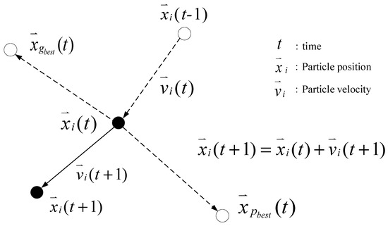
Figure 1.
Particle movement.
An individual extremum (pbest) is a particle’s optimal position in the iterative process, whereas a global extremum (gbest) is the optimal solution that comprises the optimal positions of all the particles of the particle swarm.
The particle position and velocity are updated as follows:
where and represents the ith particle velocity and location, respectively; represents the inertia weight; and are the learning factors, where usually = = 2.0 [38]; and are random numbers between 0 and 1, preventing the data from becoming stuck in local optimal solutions; p represents pbest; g represents gbest; and x indicates the current position of a particle.
3.4. Model Performance Evaluation
After the models are established, their accuracies must be evaluated and compared using various performance indicators, such as the correlation coefficient (R), the mean absolute error (MAE), the mean absolute percentage error (MAPE) and the root mean square error (RMSE). The evaluations of these indices are summarized as follows.
• Correlation Coefficient
R ranges between −1 and 1 and represents the level of association between and . An absolute value of R closer to 1 denotes a greater linear relationship between the predicted and actual variables:
where n is the number of predicted values; represents a value that is predicted from the machine-learning model and is the corresponding actual value.
• Mean Absolute Error
MAE refers to the absolute residual error between the predicted and actual values; errors do not cancel each other out so MAE accurately reflects of the range of errors:
• Mean Absolute Percentage Error
MAPE is the most commonly used indicator for assessing the quality of a predictive model. Because MAPE is a relative value and is not affected by units or numerical values, it captures differences between the predicted and actual values more objectively than other indicators do [31]. A MAPE value closer to 0 indicates more accurate model predictions:
Table 1 presents the MAPE evaluation criteria [39].

Table 1.
Mean absolute percentage error (MAPE) evaluation criteria.
• Root Mean Square Error
RMSE refers to the root mean of the sum of the squares of the residual values and captures the degree of dispersion of a sample. A smaller RMSE value indicates the higher reliability of a model:
The applicability of a classifier to a set of data can be determined by assessing its predictive performance. Most of the time, model errors cannot be accurately obtained but can only be estimated. Cross-validation is a statistical method that can be used to evaluate the robustness of a model.
When the number of available data is relatively small, the generalizability of a model is normally obtained through a 10-fold cross-validation [40]. Generally, the data are randomly grouped into a training and test data set. The data are evenly divided into ten groups, nine of which are for training and one for testing. This process is carried out ten times and the results are averaged to evaluate the applicability of the classifier.
4. Risk-Informed Simulation for Dredging Project
4.1. Collection and Preprocessing of Data
The research data that were used herein were mostly taken from documents that were obtained from the dredging management system and paper files in river management offices. Originally hundreds of projects were collected. However, only the data on 53 dredging projects were valid for subsequent analysis. During the processing of the data, extreme values and errors were identified. The abnormal cases were excluded since this investigation focused on normal conditions rather than unusual and extreme events. A total of 48 projects was thus used to establish the model in this study.
4.1.1. Data Preprocessing
During the data preprocessing, significant variability in the data was noted. The examined dredging projects differed significantly in the amounts dredged, and the related data were widely dispersed. Consequently, the data on project durations were also widely dispersed, so the direct application of the machine learning might have disfavored the stability of the prediction model. Therefore, the data were standardized to lower the variability of the variables before machine learning began and the MCS model was established.
The data were processed differently according to their characteristics. A total of five models, hereafter referred to as Duration Models 1–5, were created. Table 2 lists the preprocessing of the variables. Logarithmic transformation (Log) or min–max normalization (Min_Max) was carried out for the conversion of raw data for model experiments. The normalization function is as follows:
where denotes the numerical value after standardization; denotes the original variable in the model, and , are the minimum and maximum values of in the data, respectively.
Table 2.
Model descriptions and variable settings.
4.1.2. Feature Selection
Interviews were conducted with project coordinators in the ten river management offices in Taiwan to identify the project management situation before the model parameters were set. The interviews established that numerous risk events involved typhoons and flood seasons. Some of the regions in which dredging projects have been conducted have poor geological conditions and suffer changes in geological materials that are caused by typhoons. These incidents have prevented dredging operations from being carried out as scheduled.
Project conditions affect the bidding for the sale of dredged soil and gravel and the eligibility criteria for bidders. It discourages sellers from accepting the dredged materials and thus delays subsequent operations and inspections. Case studies and interviews with experts revealed the critical roles of the texture of soil, sand and gravel materials in dredging operations. Therefore, the proportions of sand, gravel and soil of the river in the project were selected as the variables in a quantified risk assessment model to determine their effects on the duration of a dredging project.
During the planning stage of a construction project, most project coordinators determine the price of soil and gravel materials with reference to the average prices that were applied in previous projects. Market conditions and prices that are specified in tenders affect the willingness of companies to bid, and in some regions, the market for particular materials may be saturated. Therefore, bidding using original average prices may result in a lack of bids or a tender winner. Accordingly, variables that are related to market conditions and pricing were also selected as model variables. The average price of soil and gravel was calculated by dividing the selling total prices by selling weight. The records can be found in the document of the project.
In the event of heavy rainfall during construction, the project will stop, affecting the project schedule. Therefore, the average number of rainy days per month in each basin (the number of rainfall days during the project) is obtained from the “Average Monthly Estimated Rainfall Statistics of the Central Watersheds of the Ministry of Economic Affairs” for use in the duration model.
Damage to a required road by a natural disaster during a dredging project will affect its duration. Such factors as the construction material and location of a road were used to reflect this possibility in the unit price of the road. Therefore, the estimated length of river dredging at the beginning of the project and the construction cost of roads based on the regional marketing price are taken into consideration. The river bureau uses different file formats. Therefore, the total setting and maintenance cost of the river transport road was used as another factor in the construction duration model.
After numerous discussions with experts, eight quantifiable factors concerning which historical data are available were selected for the modeling project duration. These factors used were the amounts of sand, gravel and soil as the proportions of the river, the average price of soil and gravel, the total dredging volume, the total tender cost, the number of rainfall days and the total setting and maintenance cost of transport roads.
4.1.3. Sensitivity Analysis on Influential Factors
After selecting the factors of the dredging project, an open-source machine-learning software (Weka 3.9) was utilized to perform a preliminary sensitivity analysis. Three performance indexes—MAE, RMSE, and MAPE—were adopted to evaluate the influence of distinct factors on the project duration using a linear regression model. The most influential factors on the project duration were rainfall day and total dredging volume. Considering the compositions of the dredged materials, gravel percentage was more critical than soil and sand proportions in the dredging river. Owing to the limitation of the data accessibility, only eight available factors were analyzed here. The further investigation of the influential factors, such as market condition and policy changes, should be conducted in the future. With the increased factors and amount of historical data, the proposed estimation model should be enhanced in its accuracy and reliability.
4.2. Establishment of Deterministic Project Duration Model
4.2.1. Model with Default Parameter Settings
After the data were processed, a deterministic model was established. The data, normalized using various methods, were applied to four single models (LR, SVR, CART, and ANN) with default parameter settings as shown in Table 3. After the default parameter values were set, 10-fold cross-validation was used to prevent the model from being biased toward certain training or test data, which could potentially yield erroneous simulation results. The data were evenly divided into ten groups, of which nine were used for training and one was used for testing. This process was carried out ten times. The means of R, MAE, RMSE, and MAPE were obtained.
Table 3.
Models with default parameter settings.
R, MAE, RMSE, and MAPE are statistical indicators that are frequently used to estimate errors and assess the accuracy of models. The models were finally compared to identify the best model and the optimal one was identified. Table 4 lists the performance measures of the project duration models that were developed in this study. Analytical models with poor or unreasonable performance measures were not considered, and labeled as N/A.
Table 4.
Model performance measures.
4.2.2. Model Parameter Optimization and Stability Test
MAPE is a dimensionless measure, and it provides a more objective assessment than other performance indicators of the differences between the predicted and actual values of numbers. Therefore, MAPE was adopted as the primary indicator for the assessment of the appropriateness of models in this investigation, and the other performance indicators were treated as secondary. The results revealed that SVR (Model 3) exhibited the most satisfactory performance. Therefore, PSO was carried out to optimize parameters C and γ in this model.
Before the PSO was performed, the basic parameters were set as the number of particles = 50, inertia weight (w) = 0.9, learning factor (c1, c2) = 2.0 [41,42,43] and the number of iterations = 3000. The number of iterations was set at a relatively high value because of the need for the data convergence in a Python program. Insufficient iterations produce an output value that corresponds to a locally optimal solution. Notably, the complexity of the model stability assessment increased after Duration Model 3 combined with PSO. Figure 2 presents the framework for the development of an optimized model.
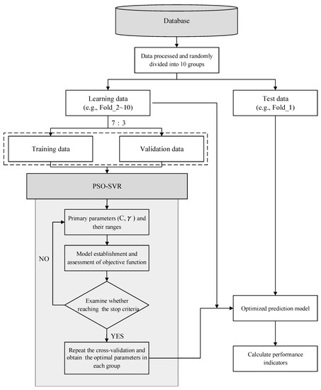
Figure 2.
Framework for the development of the optimized model.
The dredging project data were randomly divided into ten groups; the ranges of parameters were established using the PSO initial number of particles and the iterative process was run until the RMSE was minimized, yielding the optimal parameters for the model. The ranges of parameters C and γ were set at (1E-8, 1E15) and (1E-20, 1E2), respectively. They were relatively large because of the dispersion of the data. An excessively small range limits the value to the local optimal solutions rather than global optimal solutions. The parameter ranges were determined by performing several tests and assessments.
The optimized parameters were input into each group of data. Table 5 lists the results of the tests of the stability of the project duration model, which were generally found be stable even though overfitting occurred with the fourth and ninth data groups. The MAPE standard deviation for the ten data groups was calculated to be 11.09%, which was acceptable.
Table 5.
Model stability test after parameter optimization using PSO.
The output results that were obtained using the training and test data were averaged and organized in Table 6 to reveal the model performance after parameter optimization, which was compared with that using the default parameter settings. Optimizing the parameters increased R significantly (from 0.318 to 0.647), and reduced the error rate significantly, as MAE fell from 77.415 to 63.020 (days), RMSE fell from 100.234 to 76.555 (days), and MAPE declined from 27.55 to 22.93 (%). Accordingly, PSO is suitable to be used to optimize the parameters in project duration prediction model.
Table 6.
Average results of the model learning and test.
After the model stability test was completed, PSO was used to optimize the parameters of the project duration prediction model. Doing so involved firstly setting the parameter ranges. The optimized parameter ranges from the aforementioned model stability test were used in the data optimization process and the values of C and γ were optimized as 1.418530612 and 0.549995652, respectively, completing the model optimization.
4.3. Project Duration Risk Simulation
MCS is based on the law of large numbers so as to present the risk information of provided data. It was combined herein with machine learning. The factors that cause uncertainty in the project duration model were incorporated into the simulation process and a massive simulation was performed on the historical data to yield a CDF graph that represented real situations. Figure 3 shows a flow chart of this process.
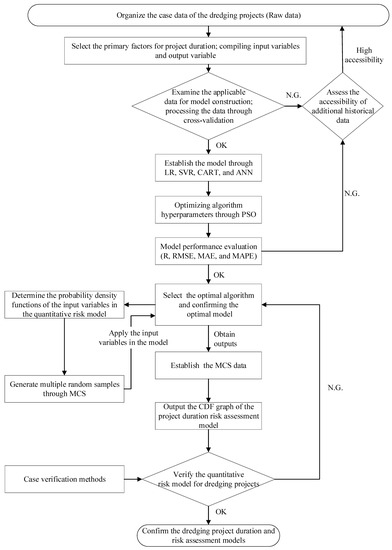
Figure 3.
Machine learning in conjunction with the Monte Carlo simulation.
4.3.1. Risk Probability Density Function of Model Variables
According to the literature review, Crystal Ball, a frequently employed statistical analysis program, was used in the MCS [44]. Crystal Ball can be jointly used with Microsoft Excel to evaluate the applicability to the distributions of the values of input variables. The program calculates and displays the applicable distributions based on the data characteristics, which are then evaluated to choose the best distribution by the users according to their needs.
After the values of the parameters were acquired, many random numbers were generated using the Scipy library in Python to call out the distribution function of every factor. The random number acquisition result was then examined using the equations for “count,” “bins,” and “ignored.” Table 7 presents the parameters of the risk probability density functions for the project duration model.
Table 7.
Probability density functions of the model variables.
4.3.2. Risk-Informed Curve
After the probability density function parameters for each variable were acquired, 500, 1000, 3000, 5000, 7500, and 10,000 pieces of data were acquired from each variable distribution (Table 7) by setting the sampled data to be non-negative values to meet the actual engineering situation. The groups of random numbers were then input into the optimized deterministic model to predict the number of days that are required to complete the dredging project. Based on the risk-informed curve that was output using the project duration model with MCS, the curve converged after the simulation was run within 10,000 times.
In the graph, the horizontal axis represents the duration for a project and the vertical axis represents the empirical probability (%). The specific values of model variables can be input to calculate the project duration (such as 350 days), based on the historical data of dredging projects that were collected from the ten river management offices. When the model suggests that a dredging project can be completed in an approximate number of days, the risk-informed curve will show the probability of the historic projects that were completed in this duration under the same conditions.
5. Development and Design of Risk Quantification System
After the project duration risk assessment model was established, a system interface was created and validated with reference to historical cases.
5.1. Background and Tools for Interface Creation
Programming is the primary task in creating the interface. Python is free, easier to use and more widely used than other high-level programming languages. It features numerous modules that programmers can apply and develop. In this investigation, Python 3.6 was used in conjunction with the Tkinter module to program the interface.
5.2. Interface Creation Process
The interface was named “Dredging Project Quantitative Risk Assessment 123.” The term “123” indicates that only three steps are required to provide the quantitative risk. The primary task of the interface was to integrate the tasks that are specified in Section 4. The Tk module was subsequently used to complete the design of the interface (Figure 4).
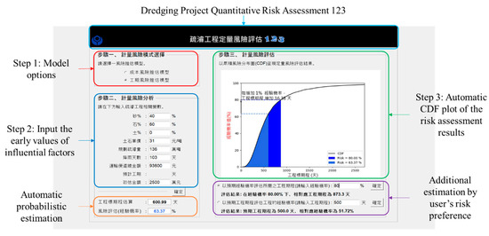
Figure 4.
System demonstration.
5.3. System Verification
Data from two historical dredging projects, provided by the river management offices, were used to verify “Dredging Project Quantitative Risk Assessment 123.” These projects were “Dredging Project at Sections 58 to 61-1 of Dajia River: Separation of Dredging and Selling of Soil and Gravel” in 2018 (hereafter referred to as Case 1)” and “Dredging Project at the Upper Streams of Maoluo River from Zushi Bridge to Nangang Bridge and Lumei Bridge: Separation of Dredging and Selling of Soil and Gravel” in 2015 (hereafter referred to as Case 2). Notably, in Case 1 the average price of soil and gravel was sixteen times higher than Case 2 and the gravel proportion was also much higher than in Case 2. However, the planned dredging volume of both cases were almost the same.
After the two cases were used for verification, the model parameters were input into the model (PSO–SVR). The model determined that Case 1 was completed in 264 days with an empirical probability of 35.90%. In fact, Case 1 was completed in 359 days. The prediction error was therefore 26.46%. The model also determined that Case 2 was completed in 387 days with an empirical probability of 64.03%. In fact, Case 2 was completed in 465 days, so the error was 16.67%.
Two cases were used to validate the project duration model, revealing that improvements are required even though the accuracy of the model in predicting project durations and calculating the empirical probability were acceptable. This result followed from the fact that a limited number of cases were considered, so insufficient references were available for the model. Moreover, the different river management offices faced different engineering problems and carried out construction projects of various scales. Therefore, the proposed system was not applicable to all the dredging projects.
5.4. System Application
Since the WRA officers make the dredging plan at the project initiation, they must estimate the project duration for tender preparation. A computing system provides the project managers with rapid and early risk information. If a newcomer who just joins the unit does not know the project background, the system introduced in this study facilitates the engineer’s quick startup. When one estimates the risk based on one’s experience, it lacks a fair evaluation of the risk. Engineers only need basic computer skills to operate the “Dredging Project Quantitative Risk Assessment 123” system with fingertips. Based on the users’ feedback, this system is considered helpful to the dredging project officers to make the appropriate reaction at the early phase by offering an additional probabilistic estimation.
6. Conclusions and Suggestions
This study established a risk-informed modeling framework for assessing risk associated with the duration of dredging projects. The primary data concerned completed dredging projects that involved the separate dredging and selling of soil and gravel. Selected factors that relate to the duration of such projects were identified by discussions with river management office personnel and experts. In this investigation, a deterministic model was first constructed through machine learning. Then, uncertainty factors were incorporated by Monte Carlo simulation. A massive simulation was then conducted with historical data to acquire a cumulative risk probability distribution of the predicted outcomes.
After the project duration risk-informed model was established, a graphical user interface was developed to facilitate its use by project coordinators in three steps. First step, choose the duration model. The second step, enter the early information of a project. The final step, make the risk assessment. The interface can be used to rapidly evaluate the quantitative risk associated with a project by anyone without programming knowledge but with a dredging engineering background. When the interface was completed, to test the applicability of the model, newly collected dredging projects were adopted to verify the system.
The primary findings and contributions of this study are as follows.
- The database that was used herein comprised a total of 48 cases and eight factors, which were the amounts of sand, gravel and soil as proportions of the river, the average price of soil and gravel, the total dredging volume, the total tender price, the number of days with rainfall, and the cost of road transport. Relatively few data were obtained because this study, to the best of our knowledge, represents the first attempt for dredging projects in Taiwan. Data integrity is inadequate because no comprehensive database exists for analysis. Future studies should involve collaboration with the WRA to ensure that each river management office uploads relevant data.
- Combining machine learning with the optimization algorithm (PSO–SVR) improved the model performance: R increased from 0.318 to 0.647; MAE decreased from 77.415 to 63.020 (days); RMSE decreased from 100.234 to 76.555 (days); and MAPE decreased from 27.55% to 22.93%. Accordingly, PSO is suitable for use with the project duration model. After PSO was conducted to optimize the model parameters, ten-fold cross-validation was performed to test the stability of the model.
- Overfitting was detected because the applicable data were insufficient; the problems that were encountered by the river management office personnel in relation to dredging differed and the considered dredging projects had different scales. Consequently, available empirical references for the model were lacking, and the model was not applicable to all the construction projects. Adding the number of days with rainfall and the cost of road transport to the already used six factors yielded an error rate of 16.36%. The two added factors strongly influenced accuracy. Accordingly, the error could be improved by adding the highly influential factors.
- The machine-learning model, combined with the MCS, was used through a graphical user interface, which presents the predictions and risk assessment to the user. To test the applicability of the model, two newly collected dredging projects were considered. The prediction errors of the model were 26.46% and 16.77% for Cases 1 and 2, respectively. Hence, the stability of the model required improvement, although the predictive accuracy was acceptable.
- The thus obtained early predicted duration can be used as a reference basis for evaluating the appropriateness of construction planning, equipment access and environmental and social issues. If the project was delayed, the continuous siltation of the river may cause overflows and floods, which affect the safety of people’s lives and properties around the riversides.
The results of this study provide a practical reference for contractors and the Water Resources Agency. Future investigations of the duration of dredging projects may refer to the procedural structure of this study and expand it by applying heuristic learning algorithms or deep learning, thereby developing a more effective machine-learning method than the one identified in this study, further improving the model in the risk assessment system. Moreover, the proposed system is suggested to be evaluated by similar datasets and compared with computing tools so as to reshape the system application in risk-informed analysis.
Author Contributions
The authors’ contributions are provided as below: Conceptualization, methodology, resources, supervision, project administration, and funding acquisition, J.-S.C.; investigation, data curation, software, formal analysis, validation, and visualization, J.-W.L.; writing—original draft preparation and writing—review and editing, J.-S.C. and J.-W.L. All authors have read and agreed to the published version of the manuscript.
Funding
This research was funded by Ministry of Science and Technology, Taiwan, grant number 107-2221-E-011-035 -MY3.
Conflicts of Interest
The authors declare that they have no conflict of interest.
References
- Makridakis, S. The forthcoming Artificial Intelligence (AI) revolution: Its impact on society and firms. Futures 2017, 90, 46–60. [Google Scholar] [CrossRef]
- Mellit, A.; Kalogirou, S.A. MPPT-based artificial intelligence techniques for photovoltaic systems and its implementation into field programmable gate array chips: Review of current status and future perspectives. Energy 2014, 70, 1–21. [Google Scholar] [CrossRef]
- Wang, Y.-R.; Yu, C.-Y.; Chan, H.-H. Predicting construction cost and schedule success using artificial neural networks ensemble and support vector machines classification models. Int. J. Proj. Manag. 2012, 30, 470–478. [Google Scholar] [CrossRef]
- Yetilmezsoy, K.; Ozkaya, B.; Cakmakci, M. Artificial intelligence-based prediction models for environmental engineering. Neural Netw. World 2011, 21, 193–218. [Google Scholar] [CrossRef]
- Salehi, H.; Burgueño, R. Emerging artificial intelligence methods in structural engineering. Eng. Struct. 2018, 171, 170–189. [Google Scholar] [CrossRef]
- Chai, H.; Zhu, S.M. Financial risk assessment of engineering projects based on Monte Carlo simulation. Proj. Manag. Technol. 2012, 11, 79–82. [Google Scholar]
- Chou, J.-S. Cost simulation in an item-based project involving construction engineering and management. Int. J. Proj. Manag. 2011, 29, 706–717. [Google Scholar] [CrossRef]
- Raychaudhuri, S. Introduction to Monte Carlo simulation. In Proceedings of the 2008 Winter Simulation Conference, Miami, FL, USA, 7–10 December 2008; pp. 91–100. [Google Scholar]
- Sadeghi, N.; Fayek, A.R.; Pedrycz, W. Fuzzy Monte Carlo Simulation and Risk Assessment in Construction. Comput.-Aided Civ. Infrastruct. Eng. 2010, 25, 238–252. [Google Scholar] [CrossRef]
- Wu, Y.W. Application of engineering project time history risk management Monte Carlo simulation. Sinotech Eng. 2010, 55–65. [Google Scholar] [CrossRef]
- Wang, Y.; Yu, C. Predicting project success using ANN-ensemble classificaiton models. In Proceedings of the 2011 IEEE 3rd International Conference on Communication Software and Networks, Xi’an, China, 27–29 May 2011; pp. 47–51. [Google Scholar]
- Gibson, G.E.; Wang, Y.-R.; Cho, C.-S.; Pappas Michael, P. What Is Preproject Planning, Anyway? J. Manag. Eng. 2006, 22, 35–42. [Google Scholar] [CrossRef]
- Wang, Y.R. Research on Applying Artificial Intelligence to the Performance of Project Predictive Project—As an example in taiwan construction project. 2010. Available online: http://ir.lib.kuas.edu.tw/retrieve/8315/992221E151053.pdf. (accessed on 1 June 2020).
- Sooksatra, V.; Rujirayanyong, T.; Pewdum, W. Forecasting final budget and duration of highway construction projects. Eng. Constr. Archit. Manag. 2009, 16, 544–557. [Google Scholar] [CrossRef]
- Cai, X.Z.; Lu, G.C.; Xu, N.N.; Jia, A.M. Application of Monte Carlo Method in Estimating the Probability of Typhoon Invasion. Atmos. Sci. 2011, 39, 269–288. [Google Scholar]
- Mitchell, R.; Michalski, J.; Carbonell, T. An Artificial Intelligence Approach; Springer: Berlin/Heidelberg, Germany, 2013. [Google Scholar]
- Li, Y.; Jiang, W.; Yang, L.; Wu, T. On neural networks and learning systems for business computing. Neurocomputing 2018, 275, 1150–1159. [Google Scholar] [CrossRef]
- Izenman, A.J. Multivariate regression. In Modern Multivariate Statistical Techniques; Springer: Berlin/Heidelberg, Germany, 2013; pp. 159–194. [Google Scholar]
- Vapnik, V. The Nature of Statistical Learning Theory, 2nd ed.; Springer: New York, NY, USA, 2013. [Google Scholar]
- Hong, J.-H.; Goyal, M.K.; Chiew, Y.-M.; Chua, L.H. Predicting time-dependent pier scour depth with support vector regression. J. Hydrol. 2012, 468, 241–248. [Google Scholar] [CrossRef]
- Chou, J.-S.; Chiu, C.-K.; Farfoura, M.; Al-Taharwa, I. Optimizing the Prediction Accuracy of Concrete Compressive Strength Based on a Comparison of Data-Mining Techniques. J. Comput. Civ. Eng. 2011, 25, 242–253. [Google Scholar] [CrossRef]
- Chen, K.Y.; He, J.H.; Xiao, H.C. Application of Support Vector Regression to Forecast of International Tourism Demand. Tour. Manag. Res. 2004, 4, 81–97. [Google Scholar]
- Hong, W.-C.; Dong, Y.; Chen, L.-Y.; Wei, S.-Y. SVR with hybrid chaotic genetic algorithms for tourism demand forecasting. Appl. Soft Comput. 2011, 11, 1881–1890. [Google Scholar] [CrossRef]
- Hong, W.-C.; Dong, Y.; Zheng, F.; Wei, S.Y. Hybrid evolutionary algorithms in a SVR traffic flow forecasting model. Appl. Math. Comput. 2011, 217, 6733–6747. [Google Scholar] [CrossRef]
- Luo, L.J.; Ding, H.F. Grain production forecasting model based on PSO-SVR. Stat. Decis. 2010, 2010, 37–38. [Google Scholar]
- Raghavendra, N.S.; Deka, P.C. Support vector machine applications in the field of hydrology: A review. Appl. Soft Comput. 2014, 19, 372–386. [Google Scholar] [CrossRef]
- Baydaroğlu, Ö.; Koçak, K. SVR-based prediction of evaporation combined with chaotic approach. J. Hydrol. 2014, 508, 356–363. [Google Scholar] [CrossRef]
- Suryanarayana, C.; Sudheer, C.; Mahammood, V.; Panigrahi, B.K. An integrated wavelet-support vector machine for groundwater level prediction in Visakhapatnam, India. Neurocomputing 2014, 145, 324–335. [Google Scholar] [CrossRef]
- Sumaiya Thaseen, I.; Aswani Kumar, C. Intrusion detection model using fusion of chi-square feature selection and multi class SVM. J. King Saud Univ.—Comput. Inf. Sci. 2017, 29, 462–472. [Google Scholar] [CrossRef]
- Patel, N.; Upadhyay, S. Study of various decision tree pruning methods with their empirical comparison in WEKA. Int. J. Comput. Appl. 2012, 60, 20–25. [Google Scholar] [CrossRef]
- Yeh, J.C.; Liu, Z.Q.J.; Dong, G.T. The Impact of Population Structure Change on Human Resources, Economic Growth and Social Welfare Allocation: A Case Study of China. J. Glob. Bus. Manag. 2011, 23–31. [Google Scholar] [CrossRef]
- Zhang, G.; Eddy Patuwo, B.; Hu, M. Forecasting with artificial neural networks: The state of the art. Int. J. Forecast. 1998, 14, 35–62. [Google Scholar] [CrossRef]
- Heidari, E.; Sobati, M.A.; Movahedirad, S. Accurate prediction of nanofluid viscosity using a multilayer perceptron artificial neural network (MLP-ANN). Chemom. Intell. Lab. Syst. 2016, 155, 73–85. [Google Scholar] [CrossRef]
- Kayarvizhy, N.; Kanmani, S.; Uthariaraj, R. ANN models optimized using swarm intelligence algorithms. WSEAS Trans. Comput. 2014, 13, 501–519. [Google Scholar]
- Karlik, B.; Olgac, A.V. Performance analysis of various activation functions in generalized MLP architectures of neural networks. Int. J. Artif. Intell. Expert Syst. 2011, 1, 111–122. [Google Scholar]
- Kennedy, J.; Eberhart, R. Particle swarm optimization (PSO). In Proceedings of the IEEE International Conference on Neural Networks, Perth, Australia, 27 November–1 December 1995; pp. 1942–1948. [Google Scholar] [CrossRef]
- Marini, F.; Walczak, B. Particle swarm optimization (PSO). A tutorial. Chemom. Intell. Lab. Syst. 2015, 149, 153–165. [Google Scholar] [CrossRef]
- Zheng, K.-W.; Wang, H.-F. A dynamic local and global conjoint particle swarm optimization algorithm. Int. J. Inf. Manag. Sci. 2014, 25, 1–16. [Google Scholar]
- Hong, Z.S. Research on Estimating Road Section Rate by Fuzzy Grouping Method. Bachelor’s Thesis, Jiaotong University, Shanghai, China, 2013; pp. 1–36. [Google Scholar]
- Singh, G.; Panda, R.K. Daily sediment yield modeling with artificial neural network using 10-fold cross validation method: a small agricultural watershed, Kapgari, India. Int. J. Earth Sci. Eng. 2011, 4, 443–450. [Google Scholar]
- Kamaruddin, S.; Ravi, V. Credit card fraud detection using big data analytics: Use of psoaann based one-class classification. In Proceedings of the International Conference on Informatics and Analytics, Pondicherry, India, 25–26 August 2016; pp. 1–8. [Google Scholar] [CrossRef]
- Bao, Z.; Watanabe, T. Mixed constrained image filter design using particle swarm optimization. Artif. Life Robot. 2010, 15, 363–368. [Google Scholar] [CrossRef]
- Ji, C.; Liu, F.; Zhang, X. Particle swarm optimization based on catfish effect for flood optimal operation of reservoir. In Proceedings of the 2011 Seventh International Conference on Natural Computation, Shanghai, China, 26–28 July 2011; pp. 1197–1201. [Google Scholar] [CrossRef]
- Saha, N.; Rahman, M.S.; Ahmed, M.B.; Zhou, J.L.; Ngo, H.H.; Guo, W. Industrial metal pollution in water and probabilistic assessment of human health risk. J. Environ. Manag. 2017, 185, 70–78. [Google Scholar] [CrossRef]


© 2020 by the authors. Licensee MDPI, Basel, Switzerland. This article is an open access article distributed under the terms and conditions of the Creative Commons Attribution (CC BY) license (http://creativecommons.org/licenses/by/4.0/).