1. Introduction
Adsorbable organic halides (AOX) are organic compounds containing halogen atoms (Cl, Br, and I) [
1,
2]. AOX are mainly formed in industrial processes using chlorine or chlorinated chemicals, such as bleaching. For example, the production of AOX is a major problem arising in the paper and pulp industries [
3]. Because AOX are unwanted side products of industrial processes, they usually end up in the resulting wastewater. AOX can have carcinogenic or mutagenic properties and should, therefore, be removed from wastewater [
4]. Conventional wastewater treatment processes are often insufficient for realizing complete AOX removal [
5]. Therefore, several other removal techniques have been proposed in the literature, including adsorption [
5,
6], biological treatment [
7,
8,
9], nano and ultrafiltration [
10,
11], and advanced oxidation processes (AOPs). AOPs employ the production of highly reactive radicals (hydroxyl radicals, *OH) to eliminate target substances through oxidation. Examples of AOPs used for AOX degradation are ozonation (alone or combined with UV irradiation) [
12], peroxone treatment [
13,
14], and Fenton oxidation [
15].
The analytical determination of AOX concentration is time-consuming and expensive. Furthermore, a real-time and continuous assessment of AOX concentration during the ozonation process could enable one to determine at which point AOX concentration has dropped below the preset limit and is hence useful as a control tool. This facilitates the optimization of the reaction time and hence the ozone and electricity consumption of the ozonation system. Therefore, the development of a more-straightforward determination method is highly desirable, preferentially via analysis tools that are (i) fast, (ii) nondestructive, (iii) environmentally friendly, and (iv) do not require any additional chemicals [
16]. Previous studies have already suggested UV-VIS spectroscopy as an adequate tool to monitor the quality of wastewater, meeting these conditions [
17]. The possibility of direct in-line and online monitoring is a big advantage that enables a fast analysis. Previous research has shown the applicability of UV-VIS as a predictor for the estimation of different wastewater parameters such as COD, BOD, TSS, and TOC [
17,
18,
19].
It is well known that datasets resulting from water monitoring usually have a multidimensional structure, containing a large number of (often multicollinear) variables, making the choice of the right modeling technique very important [
17]. To this end, different modeling techniques can be used. For example, Jiao et al. [
20] used a simple multiple linear regression model to estimate the concentration of thiophanate-methyl using UV-VIS spectroscopy [
20]. Other authors have used more complicated modeling techniques such as PCA (Principal Component Analysis) and PLS (Partial Least Square) regression using UV-VIS spectroscopy only [
21,
22]. Besides UV-VIS, other spectroscopic methods, such as fluorescence spectroscopy and near infrared spectroscopy, have also been employed [
17]. The combined use of spectroscopy and other wastewater parameters is investigated less. For example, Lv et al. [
23] used multiple linear regression to estimate the toxicity of pharmaceutical wastewater using a combination of volatile fatty acids concentrations and UV-VIS spectroscopy [
23].
The aim of this paper was to estimate the residual AOX concentration (soluble and total AOX) via modeling based on the following experimental wastewater parameters: pH, chloride concentration, Water-Soluble Organic Carbon concentration (WSOC), UV-VIS spectrum, turbidity, and Solids Removable by Filtration (SRF). A dataset was obtained by applying ozonation to transform AOX compounds into biodegradable compounds. The AOX concentration was analyzed at various time points during the ozonation process. From this dataset, the wastewater parameters suitable for model building were selected using Pearson and Spearman correlations. Modeling was done by performing stepwise multiple linear regression using forward selection, eventually obtaining a multiple linear regression model.
2. Materials and Methods
2.1. Experimental Set-Up and Wastewater Sampling
The wastewater stream investigated in this particular study originates from a chemical production process. The AOX present in this waste stream can be divided into two categories: particulate AOX and soluble AOX. The particulate AOX is removed using coagulation-flocculation, followed by flotation. When the treatment process is executed above its hydraulic capacity, some of the particulate AOX will not be removed, and hence will be present in the wastewater treatment influent, causing problems in the wastewater treatment process (the presence of soluble AOX is not an issue in this specific case). A possible solution, which enables the removal of the particulate AOX before it ends up in the wastewater influent, is the installation of an ozonation unit. Therefore, a pilot ozonation unit was placed on the plant site and ozonation was performed on effluent from the coagulation-flocculation step. Because of the fluctuating characteristics of this effluent, samples from the effluent tank were taken at various time points. This way, a comprehensive dataset could be obtained, containing data points resulting from ozonation experiments on different effluents, representing the real fluctuation in characteristics of the effluent. The ozonation was carried out on wastewater streams containing both particulate and soluble AOX. To ensure the discharge limit for total AOX (particulate and soluble AOX) is not exceeded, both parameters will be taken into account in this work. To differentiate between the soluble and particulate AOX content in the wastewater, the AOX concentration in filtered and unfiltered wastewater samples is determined. This results in the soluble AOX fraction and the sum of soluble and particulate AOX content (total AOX).
The ozonation experiments were conducted using a containerized pilot plant provided by Air-Liquide. This pilot plant consisted of an ozone generator, ozone gas analyzers, an ozone destructor, and a stainless steel reaction vessel of 250 L. The ozone generator was fed with high-grade oxygen gas and had a maximal capacity of 450 g O
3/h (5.3 w%). The ozone uptake of the reaction mixture was monitored using an ozone gas analyzer at both the inlet and the off gas. The off gas was sent through an ozone destructor unit to prevent discharge of ozone to the environment. The ozonation process was executed in batch mode. For each experiment, the reactor was filled with the wastewater effluent as previously described. During the ozonation process, wastewater samples were manually taken from the reaction tank at defined time intervals and analyzed as further specified. Because the aim is to obtain a diverse set of data points for developing and training an accurate and predictive model, the sampling time or method was varied throughout the experiments. In total, nine experiments were conducted (indicated as “Batch” in
Table S1, corresponding samples for each experiment are indicated as “Sample” in
Table S1). Depending on the sampling time, the ozone dose ranged from 0 to 4161 g O
3/m
3.
2.2. Analysis Methods
Several conventional wastewater parameters were determined conform their corresponding DIN/EN/ISO norms: pH (DIN EN ISO 10523), soluble and total AOX (DIN EN ISO 9562), WSOC (DIN EN 1484), SRF (DIN EN 872), chloride concentration (DIN ISO 15923-1), and turbidity (DIN EN ISO 7027). The UV-VIS spectrum was determined using a Specord 200 photometer from Analytik Jena AG (Jena, Germany).
2.3. Dataset
The wastewater parameters used to estimate the residual total and soluble AOX concentrations are pH, chloride concentration, WSOC, UV-VIS spectrum, turbidity, and SRF. A screening of the UV-VIS spectra was carried out to make an appropriate selection of wavelengths to prevent multicollinearity. Each sample was diluted 25 times with ultrapure water to obtain a UV-VIS spectrum below the absorbance limit. It was found that for all samples, the UV-VIS spectra followed a similar trend: for every sample, a clear peak with a maximum at a wavelength of 220–230 nm was observed. An example of a UV-VIS spectrum is shown in
Figure 1. Because of the presence of an obvious peak, it was chosen to divide the UV-VIS spectra in three regions: (i) 200–210 nm: in front of the peak; (ii) 220–230 nm: at the peak maximum; and (iii) 240–250 nm: after the peak. These regions are indicated in
Figure 1. Because the peak maximum was situated at 227 nm, the absorbance at this wavelength was selected as one of the independent variables. In order to reduce the possible appearance of multicollinearity, wavelengths in the other two regions were chosen based on their distance relative to 227 nm. In this way, the following parameters were used in the model: absorbance at 200 nm, absorbance at 227 nm, absorbance at 250 nm, turbidity, SRF, pH, WSOC, and chloride ion concentration. The used dataset is shown in
Table S1.
2.4. Model Development and Validation
The independent predictor variables were obtained by calculating both Pearson and Spearman correlations for every variable in the dataset with the dependent variables (total AOX and soluble AOX concentration). In this way, the relationship between the predictor variables and the dependent variable was elucidated. If a significant correlation was found, this independent variable was used to build the model. Thereafter, the models were obtained using stepwise multiple linear regression with forward selection. This means that the independent predictor variables were sequentially added to the model, and with each additional term, the model was tested both on the significance of each term (
p < 0.05) and on meeting the assumptions of multiple linear regression (normal distribution of residuals, homoscedasticity, no multicollinearity, and linear relationship between dependent and independent variables). The improvement of the model was monitored by calculating R
2 and adjusted R
2 values for each model, as well as the Akaike Information Criterion (AIC). It was chosen to exclude interaction terms in the model, because of the absence of a specific intuitive scientific reason to do so [
24].
After obtaining the model, 10-fold cross-validation was used to validate the model. In this type of validation, the dataset is divided in 10 sections. One of the 10 sections is chosen as “external” data section, and the other nine sections are used as training data to obtain the model. The obtained model is then validated using the external data, and the differences between the fitted and the real values are calculated. This is done 10 times, using a different section as external data set every time. All statistical analyses were performed in the statistical software RStudio [
25].
3. Results and Discussion
3.1. Dataset Exploration
The obtained Pearson and Spearman correlations for each variable in the dataset with both the total and soluble AOX concentration are shown in
Table 1 and
Table 2, respectively. These correlations indicate the association between the dependent variable and each independent variable. To perform this calculation, the null hypothesis assumes no association between these variables (both Spearman and Pearson correlations are equal to 0). This way, correlation values with a significant
p-value (
p < 0.05) imply a correlation of the predictor variable with the dependent variable different from 0. In
Table 1 and
Table 2, insignificant (
p > 0.05) correlations are marked in grey. A significant correlation was found between turbidity; SRF; absorbance at 200, 227, and 250 nm; pH, and total AOX concentration. Hence, these variables were used for model building. For the soluble AOX concentration, only the WSOC was found to be insignificant. Therefore, turbidity, SRF, absorbance at 200, 227, and 250 nm; pH, and chloride concentration were used for model building.
3.2. Obtaining the Model
Following the Pearson and Spearman correlations, the contribution of each predictor variable was tested for its significance in the predicting model. During the process of stepwise linear regression, SRF, absorbance at 250 nm, and pH were found to not have made a significant contribution and were hence removed from the model for total AOX.
The full model equation obtained for the estimation of the total AOX concentration is depicted in Equation (1). This model has an R
2 of 0.926 and an adjusted R
2 of 0.921. The dependent variable (total AOX concentration) is log-transformed to meet the homoscedasticity assumption of the model. As shown in Equation (1), the turbidity and the absorbances at 200 and 227 nm were found to contribute significantly to the estimation of the total AOX concentration. The absorbance at 227 nm was found to be significant in both the linear and the quadratic term. To prevent multicollinearity, this variable was mean-centered. Equation (1) can be transformed into a more useful equation, without centered variables and log-transformed dependent variable as shown in Equation (2).
The assumptions of multiple linear regression for this model are met.
Figure 2 and
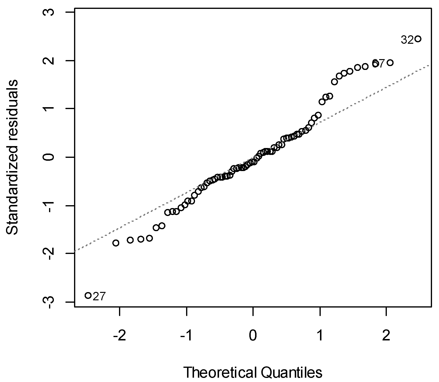
Figure 3 show the QQ-plot for the distribution of the residuals and the plot of the residuals as a function of the fitted values to test homoscedasticity, respectively. In a QQ-plot, the normality of the residuals is tested by plotting these residuals against the theoretical quantiles calculated from a normal distribution. If the residuals are normally distributed, this should result in the plot of a straight line (which is the case as seen in
Figure 2).
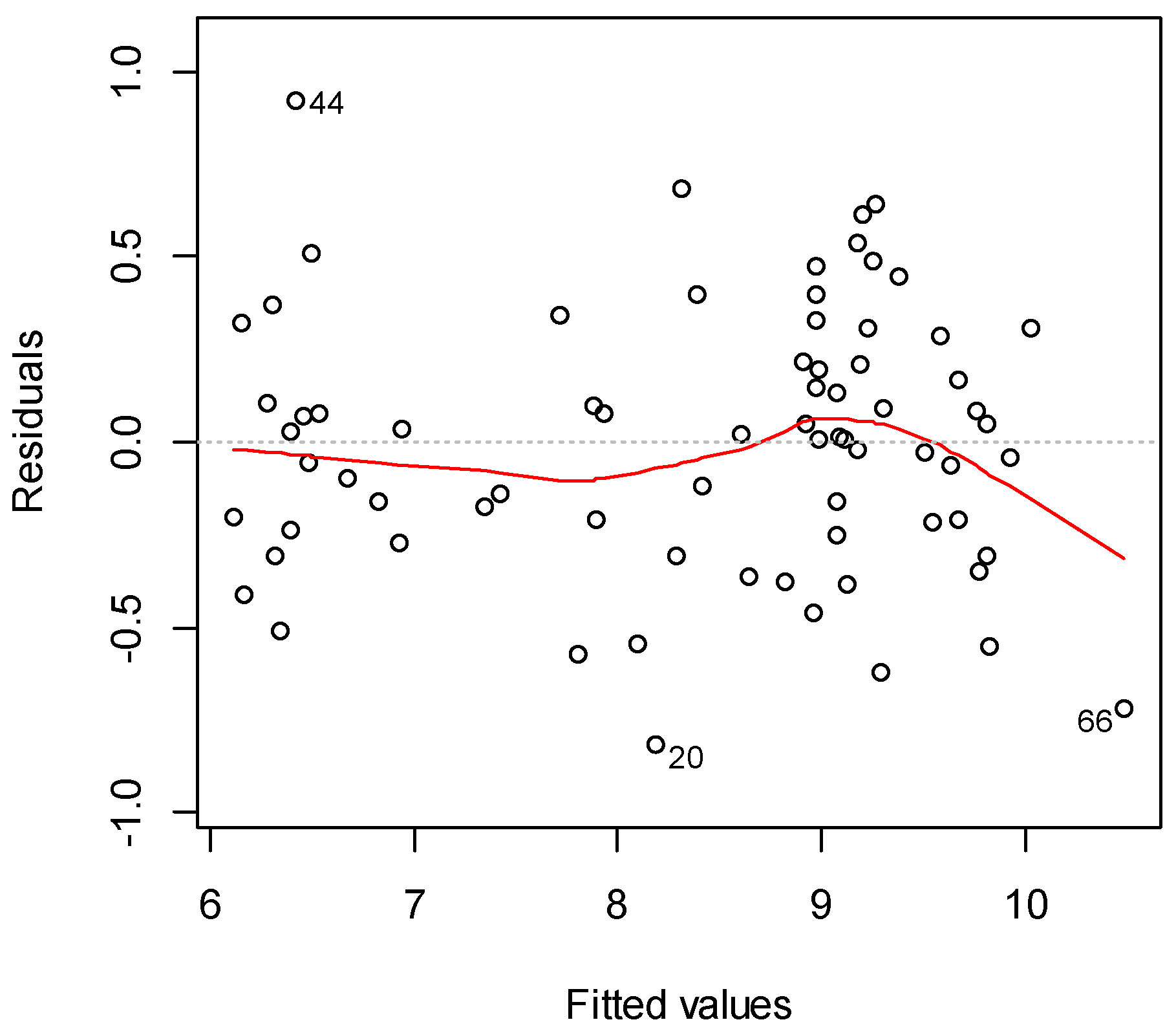
Figure 3 tests for homoscedasticity: the assumption that the variance of the residuals is independent from the dependent variable. If the homoscedasticity assumption is met, the residuals are equally distributed over the range of fitted values and no trend can be observed (the residuals do not have a specific shape). This can be seen more easily by the red line plotted in the figure, which is a LOWESS (LOcally WEighted Scatterplot Smoothing) curve. A LOWESS curve fits a smooth curve to the data (using nonparametric strategies) to give an impression of the distribution of the residuals. Ideally, when the residuals are equally distributed, the LOWESS curve should follow a horizontal line at a residuals value of zero (indicated by the dotted line). If this is the case, the positive and negative residuals balance each other out and thus are equally distributed. As can be seen in
Figure 3, the LOWESS curve is quite smooth, with a small drop at the end. This small drop can be explained by the very small number of data points in that region and the presence of a larger residual (indicated as observation 66 on the plot). Hence, the overall conclusion can be made that the homoscedasticity assumption is met. Multicollinearity was tested by calculating the Variance Inflation Factors (VIFs) for every variable.
Table 3 shows the obtained VIFs for the model. The threshold for multicollinearity was set at VIF > 2.
Similarly, turbidity; SRF; absorbance at 200, 227, and 250 nm; pH; and chloride concentration were used to obtain the model to predict the soluble AOX concentration. The modeling process identified a significant contribution of only the absorbance at 227 nm and the absorbance at 200 nm. Again, the absorbance at 227 nm was found to contribute to the model in both the linear and the quadratic term, and so this variable was mean-centered. To prevent homoscedasticity, the dependent variable (soluble AOX concentration) was log-transformed.
The full model equation for the estimation of the soluble AOX concentration is depicted in Equation (3). This model has an R
2 of 0.919 and an adjusted R
2 of 0.916. For the obtained model, the values of R
2 and adjusted R
2 are approximately equal, which indicates that the data fit the model well and all included predictor variables have a substantial influence on the dependent variable.
This results in Equation (4) for uncentered predictor variables and [soluble AOX] instead of ln([soluble AOX]).
Checking the assumptions led to the results shown in
Figure 4 and
Figure 5 and
Table 4 for testing the normal distribution of residuals, homoscedasticity, and multicollinearity, respectively. As can be seen in
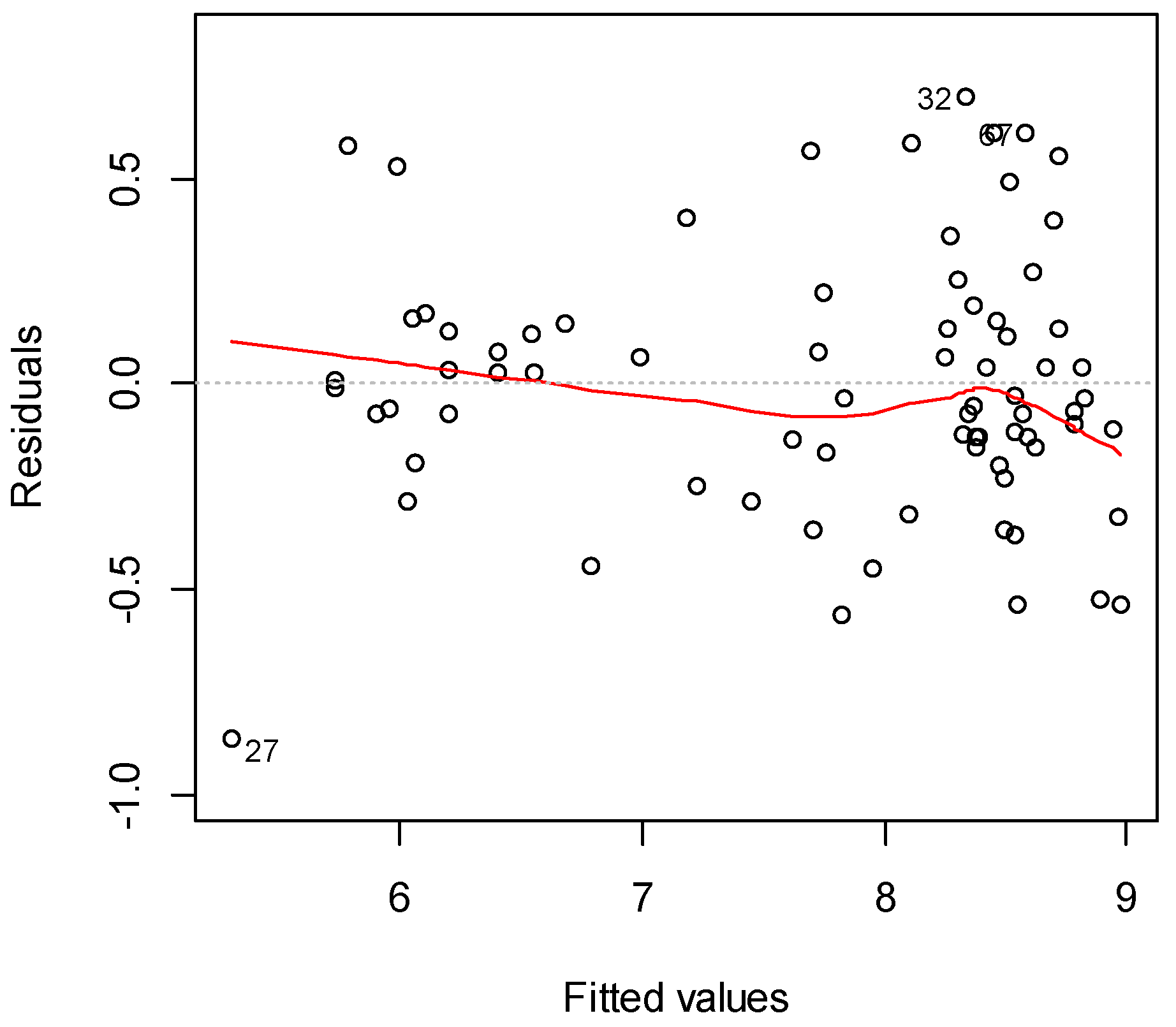
Figure 4, the data in the QQ-plot for the model for the soluble AOX concentration slightly differ from the desired straight line (especially in the upper right-hand corner). However, execution of the Shapiro–Wilk’s normality test confirmed the normality of the residuals of the model.
3.3. Validation
3.3.1. Confidence and Prediction Intervals
To evaluate the accuracy of the model, the prediction and confidence intervals were calculated. The 95% confidence interval attributes for the interval where, at specific values of the independent variables, the chance of obtaining the mean value is 95%. The prediction interval on the other hand, attributes for where an external observation is situated, considering the variability of the data matrix. There is a 95% chance that this data point is situated in this interval. Both the confidence and prediction interval per observation are shown in
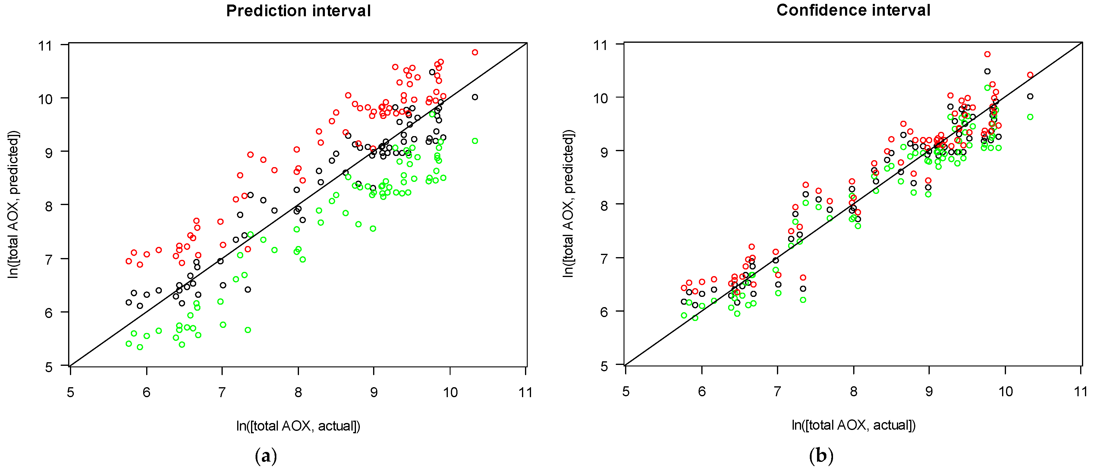
Figure 6 for the model predicting the total AOX concentration.
This figure shows a clear correlation between the predicted ln([total AOX]) and the actual ln([total AOX]) values. Only 5 out of 73 observations are situated outside ±7.5% of the predicted total AOX values. In
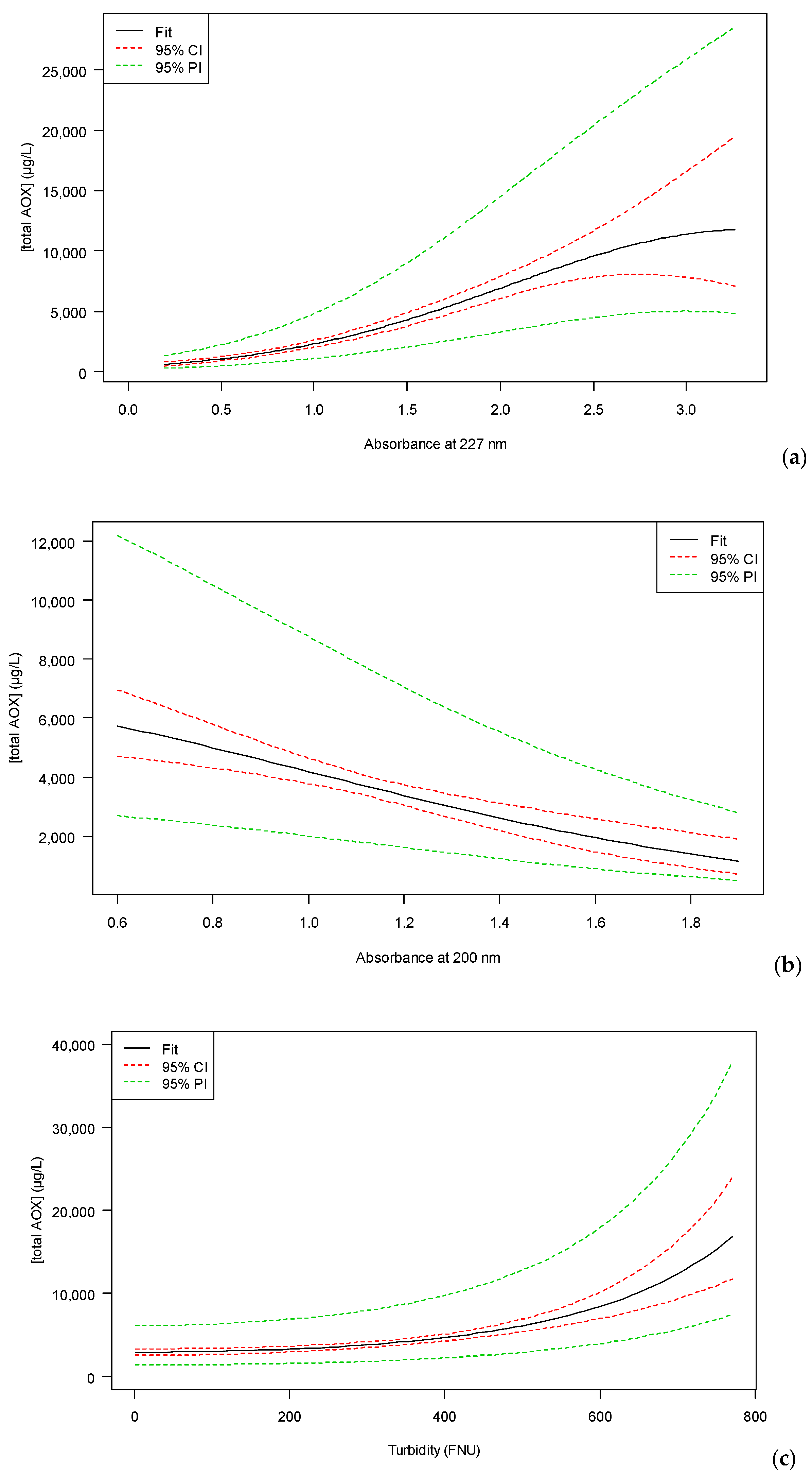
Figure 6, it is clear that both the confidence and the prediction intervals change for every observation. This is due to the difference in the values of the different predictor variables. Therefore, both intervals (confidence and prediction) were calculated for each individual parameter. In this calculation, the intervals were calculated for a change in the respective predictor variable, while the other predictor variables remained constant (mean of the predictor variable). To have a good understanding of the intervals, the obtained values were back-transformed, so the real absorbance and total AOX concentration values were obtained. The results are shown in
Figure 7. As shown in this figure, the performance of the model decreases, depending on the value of the predictor variables. In the first plot, showing the influence of the absorbance at 227 nm, it is clear that the width of the confidence interval increases rapidly at an absorbance > 2.5. In this dataset, the percentage of values of absorbance > 2.5 is 5.5%, so the probability of having a data point above 2.5 is low. Next to this, this plot is made for mean values of turbidity and absorbance at 200 nm, and this will not always be the case for observations with a high absorbance at 227 nm (similar conclusions can be drawn for all three plots). In the second plot, showing the influence of the turbidity, it is clear that the confidence interval increases rapidly (deviation of 20% from the fitted line) at a turbidity > 601 FNU. In this dataset, the percentage of values of turbidity > 601 FNU is 5.5%, so the probability of having a data point above 601 FNU is low and the conclusion is similar to that of the absorbance at 227 nm. In case of the absorbance at 200 nm, the confidence interval increases (deviation of 20% from the fitted line) at absorbances lower than 0.675 and higher than 1.4. The percentage of values of the dataset in this range is 8.2%, so the same conclusion can be made.
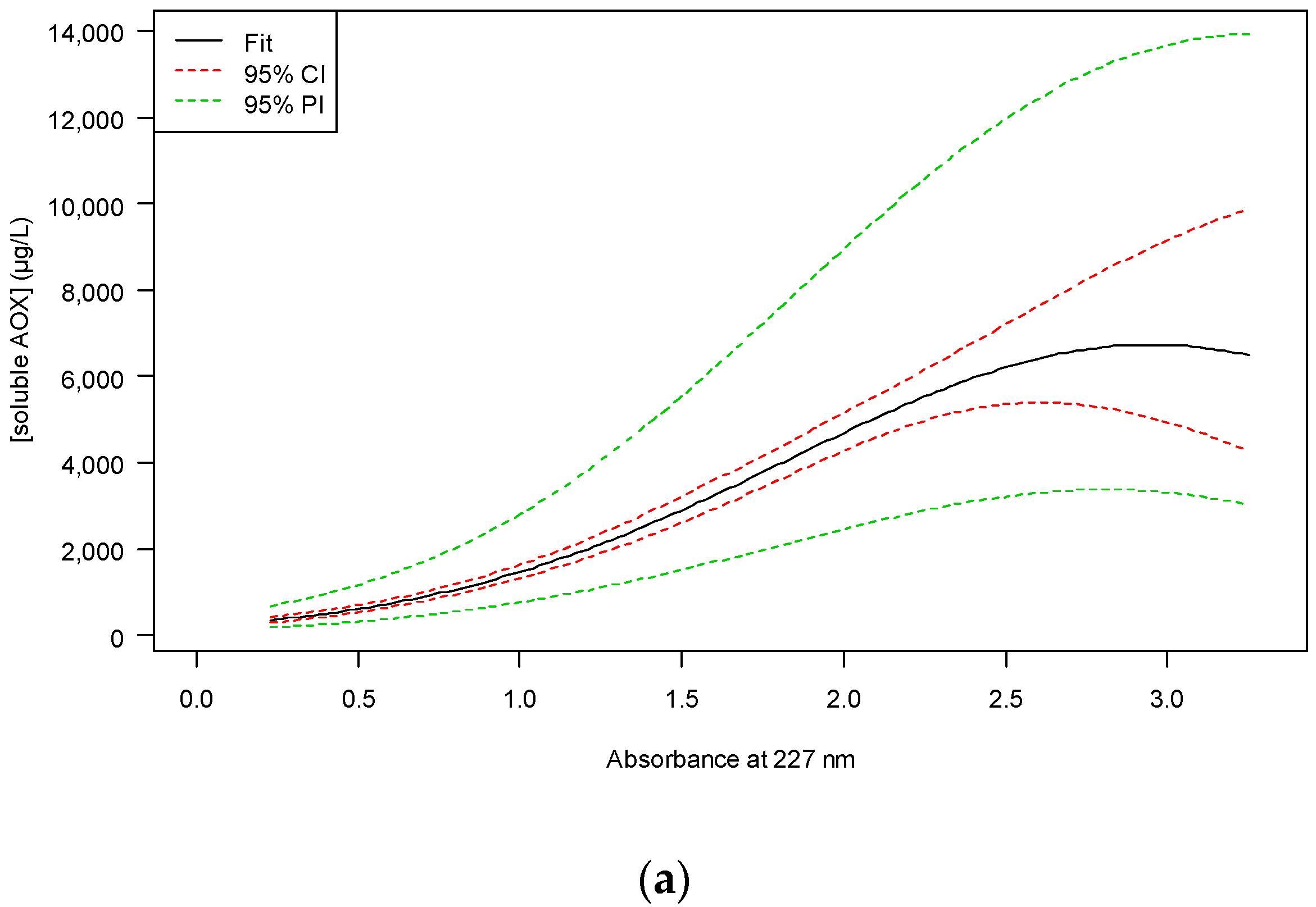
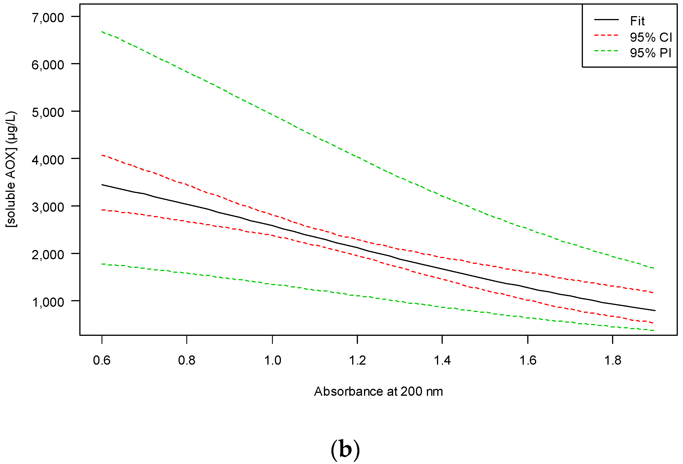
Figure 8 shows the prediction and confidence interval per observation for the model obtained for predicting the soluble AOX concentration.
These figures show a clear correlation between the predicted ln([soluble AOX]) and the actual ln([soluble AOX]) values, which indicates a good model fit. Only 4 out of 76 observations are outside ±7.5% of the predicted soluble AOX values. Similarly, as previously specified, both intervals (confidence and prediction) can be calculated for the prediction of the soluble AOX concentration, for each individual parameter. The results are shown in
Figure 9. In the first plot, showing the influence of the absorbance at 227 nm, it is clear that the confidence interval increases rapidly at an absorbance > 2.5. The percentage of values of absorbance > 2.5 in this dataset is 5.3%, so the probability of having a data point above 2.5 is low. In case of the absorbance at 200 nm, the confidence interval increases (deviation of 20% from the fitted line) at an absorbance > 1.525. The percentage of values of this dataset in this range is 2.6%, so the same conclusion can be drawn as above.
3.3.2. Cross-Validation
10-fold cross-validation was carried out to assess the performance of the model. The results are reported as the mean square error between the fitted and the real values. For the model obtained for the total AOX concentration, a mean squared error of 0.146 (log-transformed) was obtained. To visualize this error, the fit ± mean squared error (back transformed) can be added to the plots showing the confidence and prediction intervals. This is shown in
Figure S1. In these plots, the fitted interval for cross-validation lies close to the 95% confidence interval of the plots.
Cross-validation resulted in a mean squared error of 0.114 (log-transformed) for the soluble AOX concentration. To visualize this error, the fit ± mean squared error (back transformed) is added to the plots showing the 95% confidence and prediction intervals (
Figure S2). A similar conclusion can be made: the cross-validation interval lies close to the 95% confidence intervals.
3.4. Influence of Predictor Variables
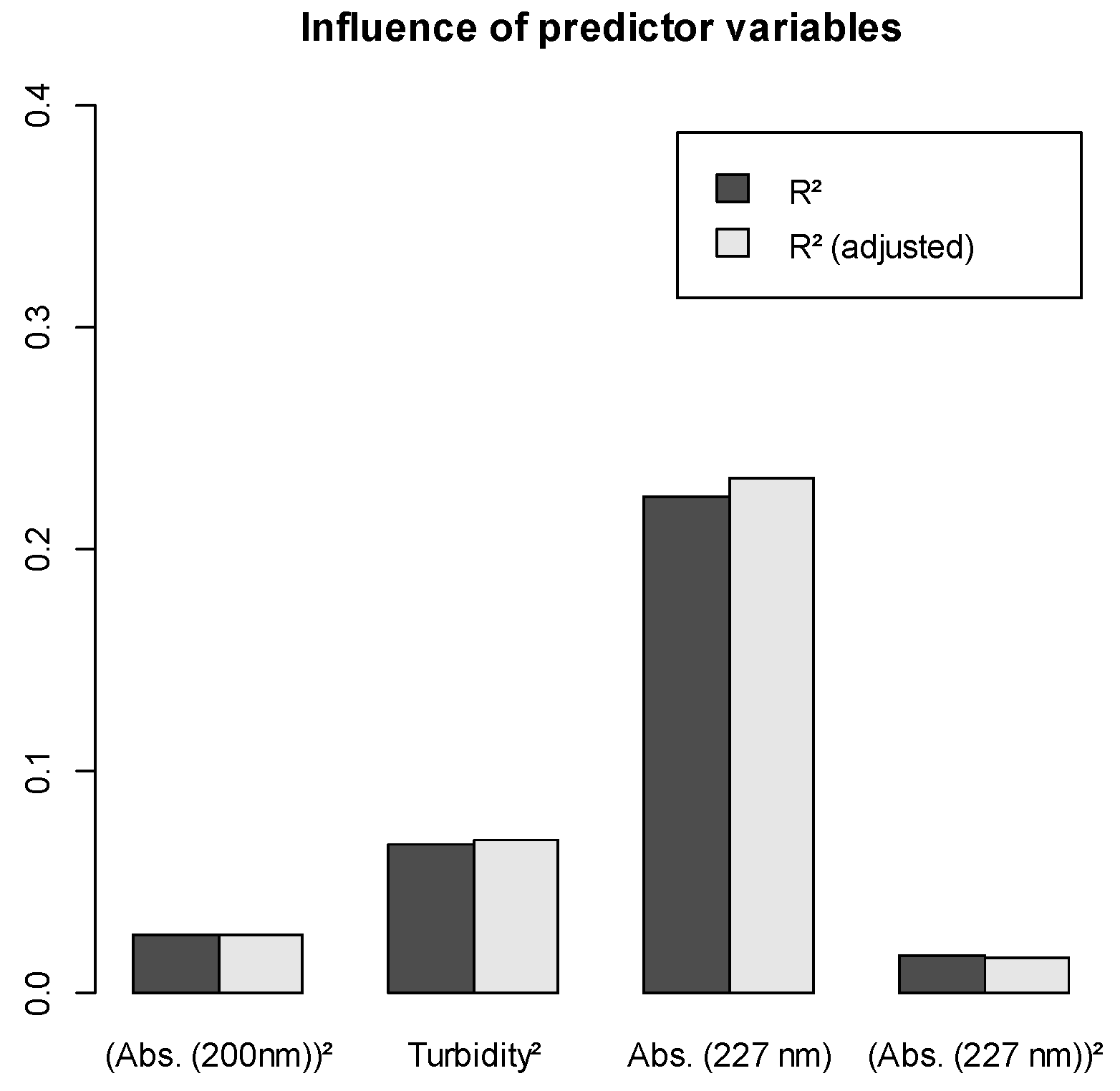
The influence of the predictor variables on the model predicting the total AOX concentration can be assessed based on their individual contribution to R
2 and adjusted R
2. These contributions were obtained by calculating the R
2 and adjusted R
2 of the model, leaving one predictor variable out of the model. The obtained R
2 and adjusted R
2 were then subtracted from the R
2 and adjusted R
2 obtained with the full model. This was done for all predictor variables. The result is shown in
Figure 10. The influence of the variables can be ranked as follows (from high to low): Abs. (227 nm)–Turbidity
2–(Abs. (200 nm))
2–(Abs. (227 nm))
2.
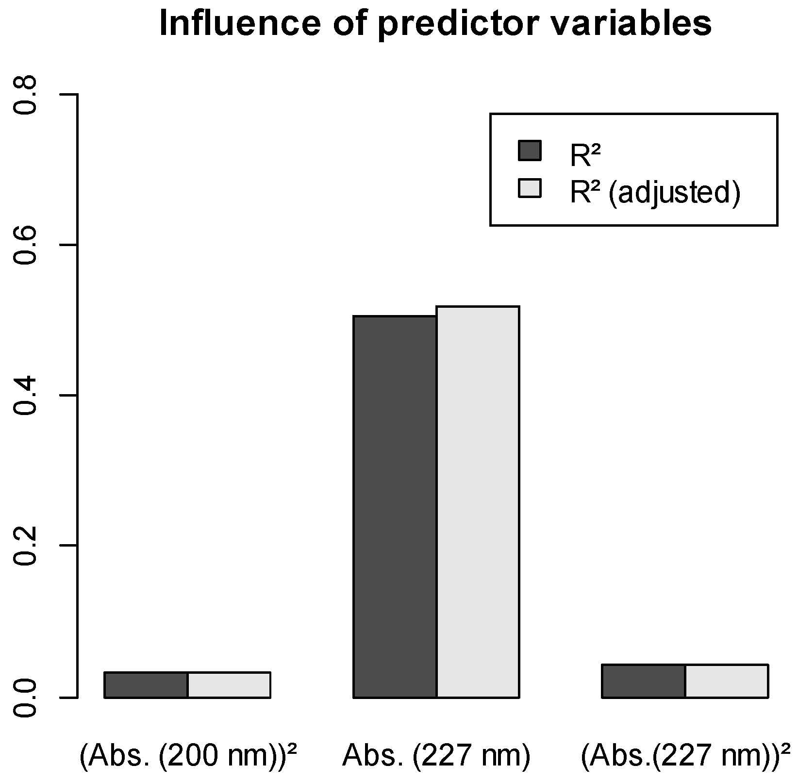
The influence of the predictor variables for the model predicting the soluble AOX concentration was assessed similarly and is shown in
Figure 11. The influence of the variables can be ranked as follows (from high to low): Abs. (227 nm)–(Abs. (227 nm))
2–(Abs. (200 nm))
2.
The similarities as well as the differences in influence of the parameters between both models can easily be explained. In both models, the absorbance at 227 nm is the most influential parameter. This wavelength corresponds with the maximum of the absorbance peak of the wastewater samples. For the model of the total AOX, the turbidity is also of importance. This can be explained by the presence of both soluble and particulate AOX in these samples. The presence of the particulate AOX has a big influence on the turbidity of the wastewater, whereas these suspended particles are filtered out in the soluble AOX samples. This explains the presence and absence of these parameters in the model for the total and soluble AOX, respectively. For the absorbance at 200 nm, no direct explanation can be found. During the ozonation process, the organic compounds present in the wastewater stream are oxidized and transformed into other organic compounds, which can readily influence the UV-VIS spectrum and can influence the absorbance at 200 nm.
4. Conclusions
An accurate model for the prediction of the total AOX concentration, meeting all model assumptions, with an R2 of 0.926 and an adjusted R2 of 0.921 was developed, containing the UV absorbance at 227 nm, the UV absorbance at 200 nm, and the turbidity of the wastewater. Confidence and prediction intervals were reported. Next to this, cross-validation was carried out to validate the model and the influence of the predictor variables was assessed.
A similar methodology for the prediction of soluble AOX was followed. An accurate model, meeting all assumptions, with an R2 of 0.919 and an adjusted R2 of 0.916 was found, containing the absorbance at 227 nm and the absorbance at 200 nm of the wastewater. Similarly, confidence and prediction intervals were reported and cross-validation was carried out. The most influential predictor variables were also defined.
These models can be beneficial for the wastewater treatment process in many ways. In first instance, the sampling frequency necessary for process monitoring can be minimized to the minimal required amount, because in-line monitoring of the UV-VIS spectra and turbidity will be sufficient for the determination of both soluble and total AOX concentrations. Secondly, the fast prediction of the AOX concentration can be useful for the optimization of the ozone dosage in the ozonation step. Currently, ozonation is carried out using a fixed ozone dose and fluctuations in AOX concentrations are resolved by applying an ozone overdose. Working at an ozone overdose can be omitted with the provided in-line monitoring system, because the ozone dosage can more easily be altered by a fast and easy determination of the residual AOX concentrations.

 ,
, 


