Abstract
In semi-arid regions, where hydrological resources are very vulnerable and where there are water shortages in many regions of the world, it is of great importance to assess the vulnerability that a system is facing or will face to the potential impacts of climatic changes and changes on the use of land. For that reason, this research focuses on evaluating the global vulnerability of a hydrological basin, taking into consideration these changes. Being different from the existing methodologies that assess the vulnerability, our methodology interconnects through a new interface a distributed hydrological model, global climate models, climate change scenarios, land use change scenarios and the largest number of system variables calculated with information from official sources. Another important point of our methodology is that it quantifies the global vulnerability of the system, taking into consideration hydrological, environmental, economic and social vulnerabilities. The results obtained show that the proposed methodology may provide a new approach to analyze vulnerability in semi-arid regions. Moreover, it made it possible to diagnose and establish that the greatest current and future vulnerabilities of the system are the result of activities in agricultural areas and urban centers.
1. Introduction
Vulnerability is a concept that emerges as a necessity for climate science and policies in the face of the potential impacts of climate change. During the last decade, the efforts to assess vulnerability to the potential impacts of climate change have contributed to the development of theories and assessment methodologies that can be found in the reports of the Intergovernmental Panel on Climate Change (IPCC) [1]. The IPCC defines vulnerability to climate change as a function of a system exposure and stimuli-response to climate and its ability to adapt to these effects [2]. According to [3], vulnerability is an indicator of possible future damages. Historically, the term “vulnerability” has been used in several contexts, such as: food security [4,5], livelihood [6], natural disasters [7] and general risk management [7,8]. In that same context, climate change has caused global concern due to adverse effects on the global ecosystem, the economy and society [9]. Therefore, in recent years, the tendency has been to assess the environmental [10], economic [11] and social vulnerability [10,11]. Other studies have focused on assessing the world’s hydrological vulnerability to the possible effects of climate change, such as those carried out by [12,13]. The foregoing is due to considering that inland water resources have been identified as one of the most important global change problems [14]. According to [1], assessing vulnerability to the potential impacts of climate change has the objective of developing policies that reduce the risks associated with climate change. According to [15], climate change has become a threat by applying greater pressure on already stressed hydrological systems and resources. Moreover, in the last decades, the impacts of climate change have already been visible, mainly in the increase of temperatures, and the increase and/or decrease of rainfall in several regions of the world [16,17]. According to [14], these impacts are of extreme importance, considering that the hydrological resources are very vulnerable, and that at present, many regions of the world face water scarcity. Under this reality, it is transcendental to estimate the vulnerability that a system is currently facing or will face taking into account future changes [18]. It is for that reason that this article focuses on assessing hydrological, environmental, economic and social vulnerability in a spatially distributed global context. Global vulnerability combines and distributes at the cell scale the four types of vulnerability described above, in which hydrological, economic, social and environmental factors converge.
According to [19], when analyzing different studies, we can observe that the methodology mostly used to quantify the vulnerability of a system by is using a composite index that includes a set of indicators. The same authors comment that these indicators represent the vulnerability of a system and are mathematically combined into a single composite index. A composite index may be easier to interpret than the tendencies of single indicators [19]. In literature, different methodologies might be found to quantify the composite indicator, such as: multiple linear regression models [20], principal components analysis and factor analysis [21], neutralization of correlation effect [22], distance to targets [23], distance to objects [23], experts opinion [24], public opinion [25], spatial multi-criteria analysis [26], Analytic Hierarchy Process [27], Bayesian model [28], Artificial Neural Networks [29], and fuzzy logic techniques [29]. According to [15], the vulnerability calculated using the existing methodology does not consider all the variables involved in the system, thus, limiting its accuracy.
In the same context, the methodologies do not introduce land use change in the vulnerability assessment. According to [30], the impacts of land use change (Urbanization) on a hydrological system produce an increase in volume and surface runoff rate, causing a decrease in groundwater recharge and base flow. According to [31,32], the land use change and climate change have been identified as two of the main factors affecting the ecosystem services. Studies like that of [33] highlight the importance of using land use change in the environmental assessment. For that reason, the authors consider to include it in the quantification of the global vulnerability. In addition, we believe that land use change will have an important effect, because the study area is located in a region where availability studies accentuate a shortage of water resources and over-exploitation of groundwater. Finally, the hypothesis of this article is that the vulnerability of a basin to the potential impacts of climate change and land use change can be evaluated through the connection of mathematical tools that will contribute to decision making, with the aim of mitigating the impacts and knowing the resilience of the system.
2. Case Study
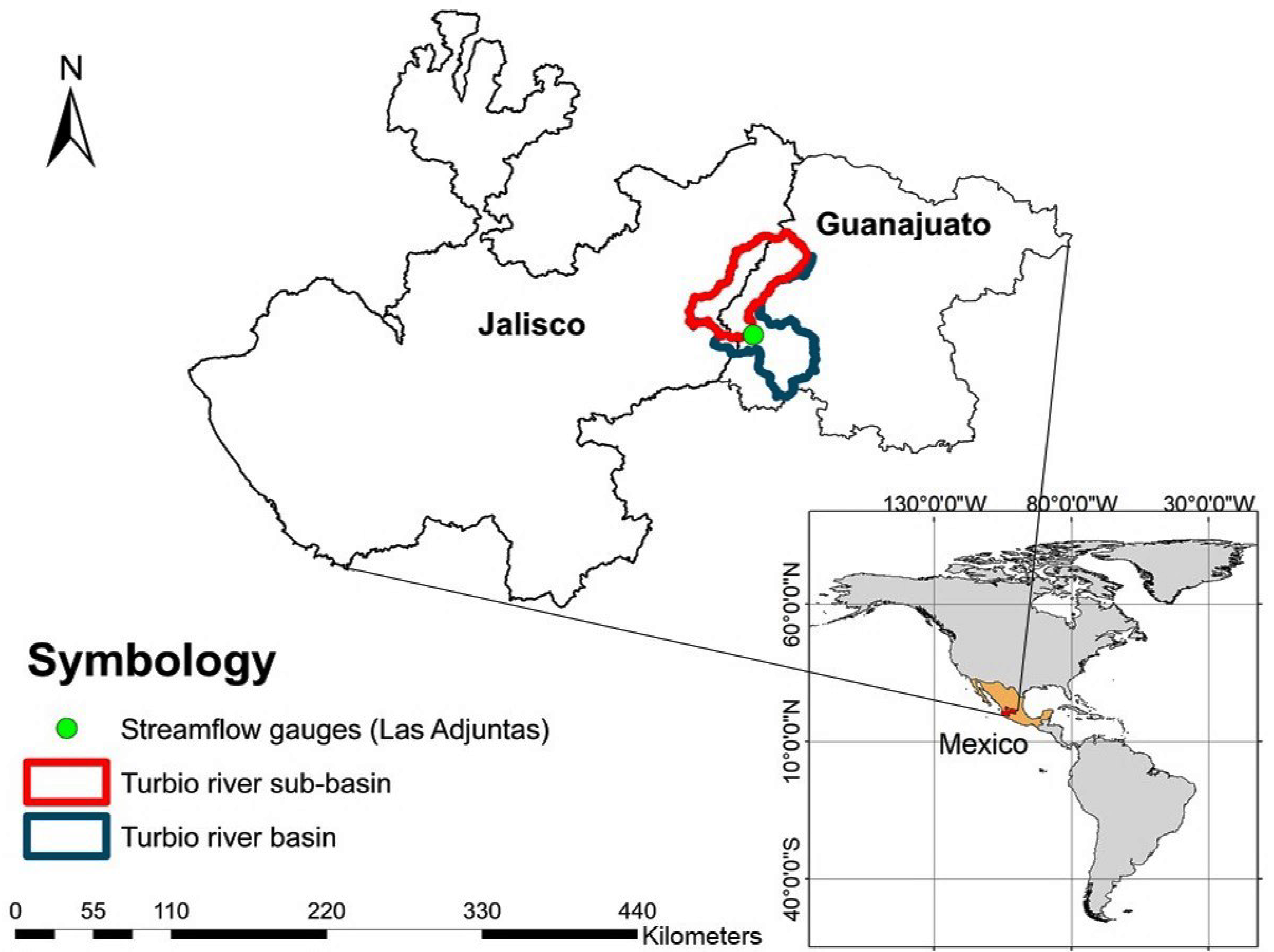
The study area used in this research is the Turbio river sub-basin (Figure 1). The sub-basin is located in the Lerma Santiago Hydrological Region, which includes the states of Guanajuato and Jalisco in Mexico. The sub-basin has an area of 2983 km and is one of the most important for agricultural production of the country.
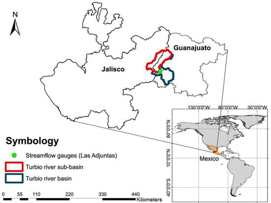
Figure 1.
Location of the Turbio river sub-basin used as a study area.
The sub-basin is located between elevations 1726 and 2872 m. Accumulated average annual rainfall varies from 560 to 807 mm, with a very marked seasonality of the rainy season and an occurrence of 90% between the months of June and September. The maximum average temperature is 25.59 °C and the minimum average temperature is 9.56 °C. The variations in temperatures have a significant influence on evaporation rates in the study area with rates ranging from 0.25 mm day to 12.45 mm day.
In the last three decades, the Turbio river sub-basin has presented problems of over-exploitation of surface and groundwater. This is due to the population growth and increased agricultural activity, supplied with surface and groundwater. This over-exploitation has generated great uncertainty among decision-makers about the future of water availability in the sub-basin, and how it will be affected by the potential effects of climate change. This scenario makes our methodology more relevant, as it aims to respond to the concerns, such as the future of water availability from the point of view of hydrological, environmental, economic and social vulnerability.
3. Methodology
In contrast to the existing methodologies, in this article, a totally different new methodology is proposed, which combines a distributed hydrological model, global climate models, climate change scenarios, land use change scenarios and the largest number of system variables calculated on the basis of information provided from official sources. Another important point of our methodology is that it quantifies the global vulnerability of the system, taking into consideration the hydrological, environmental, economic and social vulnerability. It is important to emphasize that nowadays there are no studies that consider all the vulnerabilities (i.e., hydrological, environmental, economic and social) in the assessment of global vulnerability, connecting several mathematical models in a hydrological basin. This makes our methodology new with respect to the existing ones. In addition, the effects of land use change are included in the evaluation.
The methodology that we propose to carry out this research has included the development of a Predictive Vulnerability Interface that we have called MPDV1.0. It has been programmed in Visual Basic (Microsoft, Washington, DC, USA) language and allows quantifying the hydrological, environmental, economic, social and global vulnerability of a hydrological basin. MPDV1.0 integrates the distributed hydrological model TETIS [34,35], the Global Climate Models (GCM) of the Inter-Comparison of Coupled Models-Phase 5 (CMIP5) Project [36], and RCP4.5, RCP6.0 and RCP8.5 scenarios of the Intergovernmental Panel on Climate Change (IPCC) [37]. The foregoing is following the scheme shown in Figure 2. Unlike the methodologies proposed by [38,39,40,41], MPDV1.0 calculates vulnerability in a distributed way, including all the processes and storages of the hydrological cycle through its modeling in TETIS. In addition, the effects of climate change and land use change are included as well. In the hydrological modeling with TETIS, the future land use changes are introduced, estimated with the Terrset software (Clark Labs, Worcester, MA, USA) [42]. This makes the MPDV1.0 a different and innovative way of estimating vulnerability. Another difference from the existing methodologies is that it allows quantifying five types of vulnerabilities (i.e., hydrological, environmental, economic, social and global).
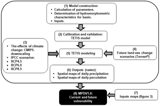
Figure 2.
Conceptual scheme of the connection of models, executed in the MPDV1.0.
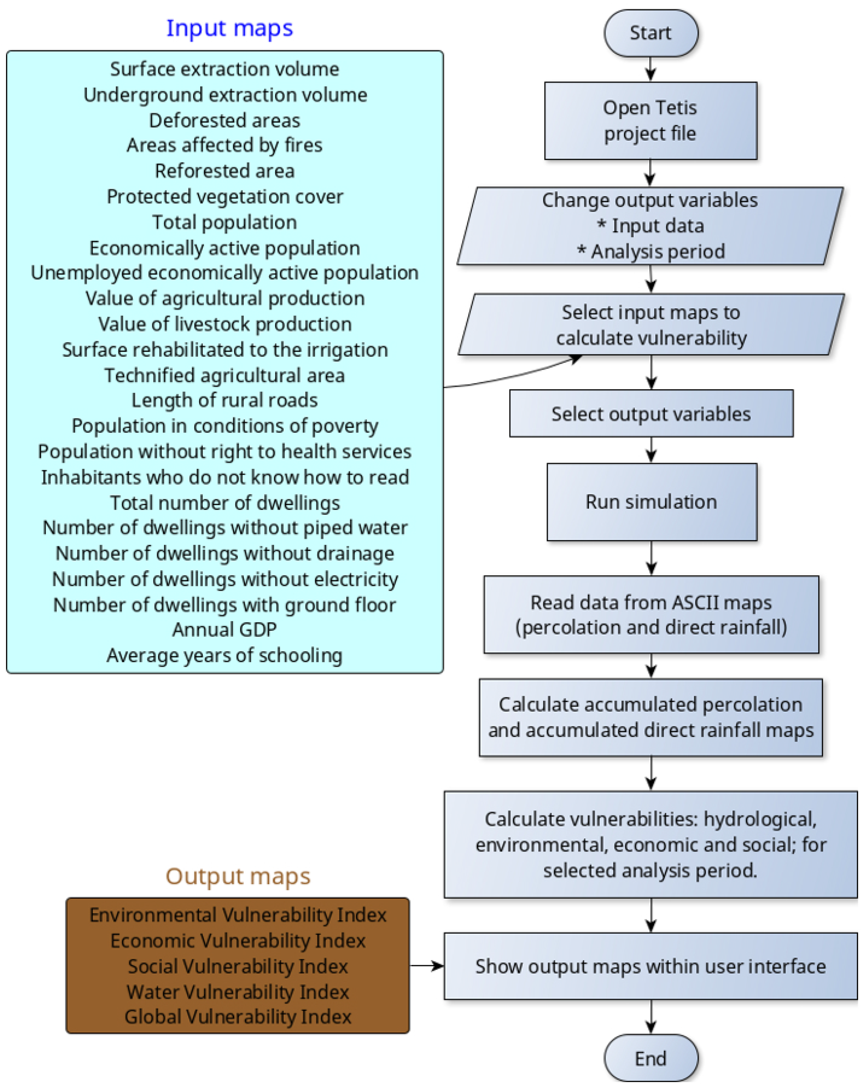
The MPDV1.0 executes the connected tools and the input maps following the flowchart shown in Figure 3. The input maps have been processed in ArcGIS (ESRI, Sacramento, CA, USA), considering the available information, obtained from different governmental departments. In the research, the error on the model and calculation of vulnerability is not estimated because the input maps are official information in Mexico and are carefully validated. These maps are introduced in ascii format in the MPDV1.0. The MPDV1.0 conducts information cross-checks to obtain hydrological, environmental, economic, social and global vulnerability.

Figure 3.
Flow chart of vulnerability modeling with the MPDV1.0.
The MPDV1.0 calculates global vulnerability, based on the IPCC’s conception of vulnerability [43], which generally explains vulnerability by applying the following equation:
where is the global vulnerability, is the hydrological vulnerability, is the economic vulnerability, is the social vulnerability, is the environmental vulnerability and n is the number of vulnerabilities. The vulnerabilities of the Equation (1) are obtained through the indicators shown in Table 1. Each vulnerability map will be calculated from the normalized indicators involved and their corresponding weights with the following equation:
where is the normalized indicators i, is the weight of the normalized indicator i and n is the number of indicators for each type of vulnerability. The indicators are normalized to eliminate the units and to vary the values from 0 to 1. The equations implemented to perform the standardization are the following:
where , and are the minimum and maximum values of the data set . If the indicator has the capacity to adaptation, Equation (3) shall be used; and If the indicator has a degree of exposure or sensitivity, Equation (4) shall be used. For each normalized indicator, a weight will be obtained using the following equation:
where is the standard deviation of the set of the indicator values i, and n is the number of selected indicators.

Table 1.
Equations and sources of information used in the calculation of indicators [44].
In this research, the MPDV1.0 has been applied to obtain present and future vulnerability maps (for the year 2035). The foregoing is with the purpose to assess the potential impacts of climate change and land use change.
3.1. Data Sets
The geographic information used in estimating the indicators (Table 1 has been obtained from the National Institute of Statistics and Geography (INEGI) available on https://www.inegi.org.mx/ and from the National Water Information System of the National Water Commission (SINA-CONAGUA) available on http://sina.conagua.gob.mx/sina/. They are governmental departments that allow free downloading of information at scales of 1:50,000 and 1:250,000.
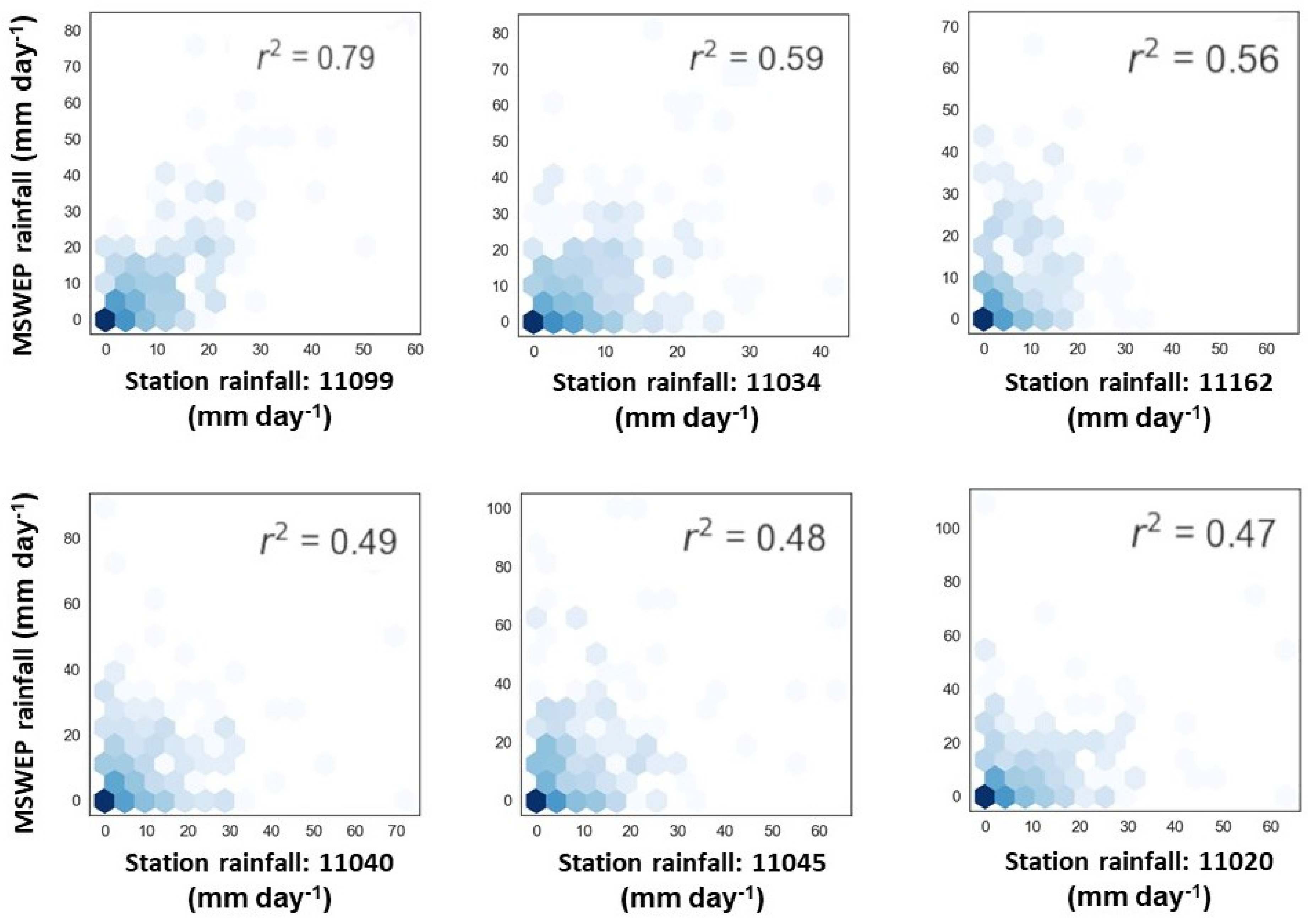
Hydrological modeling calibration has been conducted using daily flow data measured at Las Adjuntas gauge, which is located at the mouth of the sub-basin (Figure 1). These hydrometric data are also freely downloaded from the website of CONAGUA National Data Bank of Surface Waters (https://www.imta.gob.mx/bandas). In the case of precipitation data, it was initially tested using daily data from 20 weather stations. However, the first results showed some inconsistencies in the interpolation of vulnerability maps, because spatial interpolation of daily rainfall gauge data using Inverse Distance Weighting in the TETIS model has shown errors of overestimation in rainfall interpolated in the cells adjacent to the border of the basin. Moreover, the results showed the formation of bull’s-eye patterns produced by the spatial location of the weather stations. That is, the isohyets are circular in the stations without nearby neighbors, denoting a poor spatial distribution of the weather stations. To support the above, we decided to use the Multi Source Weighted-Ensable Precipitation (MSWEP) product from Princeton Climate Analytics, available on https://platform.princetonclimate.com/PCA_Platform/index.html. MSWEP is a precipitation mesh with a spatial resolution of 0.25 and a temporal resolution of three hours [45,46,47,48]. MSWEP data have been correlated with daily rainfall, observed at weather stations for the period from October 2010 to September 2014. The foregoing is with the purpose of validating the product data and justifying its use. Figure 4 shows some examples of the obtained results; in general terms, the correlations from 0.5 to 0.8 were obtained. In the case of satellite rainfall products, correlation coefficients greater than 0.5 are considered acceptable [9,49].
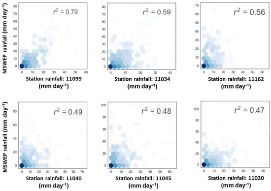
Figure 4.
Correlations obtained between MSWEP and the daily observed precipitation data.
Despite the overestimates observed in Figure 4, we decided to use the MSWEP, because the interpolated rainfall from the weather stations presents 13.5% overestimates in cells far from the stations compared to the MSWEP. We also evaluated in the analysis period the differences in the annual average accumulated precipitations and we obtained that the observed precipitations are greater than those of the MSWEP with an average of 175 mm year. There are other products with precipitation information, such as: NOAA CPC Morphing Technique (CMORPH), Integrated Multi-satellite Retrievals for GPM (IMERG) and Climate Hazards Group Infrared Precipitation with Stations (CHIRPS). Studies such as those carried out by [46,50,51,52] consider these high-precision products and have been implemented in various regions, obtaining correlations of 0.65 to 0.8. However, the information period for these products is limited. Therefore and considering the MSWEP has a longer reporting period and that similar correlations are obtained, we have decided to use it in the research.
In the hydrological modeling, 36 cells of the MSWEP product were selected; their centroids have been named “virtual stations”. By interpolating the precipitations of these stations in the period from October 2000 to September 2017, we obtained the distribution of accumulated average annual precipitations shown in Figure 5a. Figure 5b,c show the distribution of elevations in the sub-basin, the variation of precipitation in the high areas is due to an effect of latitude.
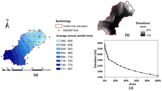
Figure 5.
(a) Accumulated average annual rainfall obtained using Multi Source Weighted-Ensable Precipitation (MSWEP) product information, (b) Digital Elevation Model and (c) hypsometric curve.
3.2. Automatic Calibration of the TETIS Model
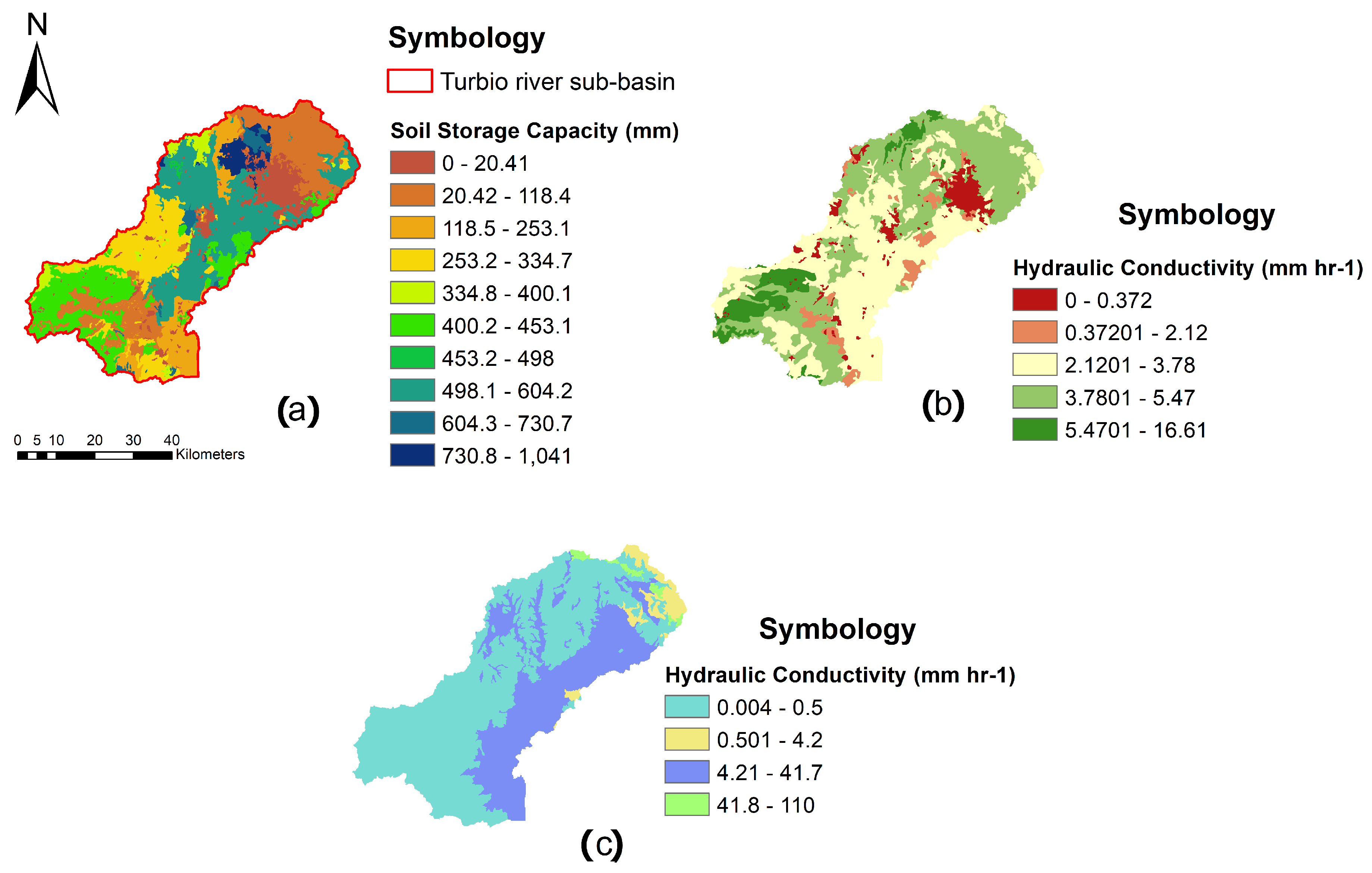
The TETIS model uses nine initial parameters (Table 2), Figure 6 shows the three most important parameters, calibrated automatically through Correcting Factors (FC). For more information on the initial parameters of the TETIS model, see for example [34,35,53].

Table 2.
CMIP5 models used for the projection of the precipitation and temperature.
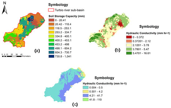
Figure 6.
(a) Static storage (Hu), (b) soil hydraulic conductivity (Ks) and (c) hydraulic conductivity of rocky extract (Kp).
The optimization algorithm used is the Shuffled Complex Evolution (SCE-UA), developed at the University of Arizona [13,54,55]. The SCE-UA obtains better performances, given that it requires less iterations to reach optimum and it is more suitable for non-expert users, while Simplex, which is a more efficient algorithm, needs a step-by-step process supervised by an expert modeler. We decided to use as an objective function, the Nash-Sutcliffe Efficiency Index (NSE), because it is the most used in hydrological model calibration [56]. The NSE is calculated using the following equation:
where is the observed flow, the simulated flow and is the mean flow observed.
3.3. Downscaling Climate Model
In this research, we decided to use the CMIP5 GCMs because they are the most used models from the end of the eighties [57,58]. Moreover, according to [59], the CMIP5 models have a better performance to represent numerous phenomena include extreme precipitation, diurnal variations in precipitation and tropical cyclone intensity. Studies such as the one carried out by [60] have shown that climate models in CMIP5 are better in future projections, because the efforts of CMIP5 are enormous, with a larger number of more complex models run at higher resolution, with more complete representations of external forcings, more types of scenario and more diagnostics stored. The projections with the GCMs have been obtained using the Climatic Atlas platform developed by the Center for Atmospheric Sciences of the National Autonomous University of Mexico and are available on https://atlasclimatico.unam.mx/AECC/servmapas. This platform was developed exclusively for Mexico considering the models shown in Table 2. It allows calculating projections using each model individually and using the 15 models together. We decided to use them together through the Reliability Ensemble Averaging (REA) conducted by [61]. According to [62], the REA reduces the uncertainty in the projections by giving greater weight to the GCMs that present the smallest errors and biases with respect to the variables observed in a given mesh point. According to [61], the weight assigned to each model is based on two criteria, (1) trend (difference with observations) and (2) convergence (difference between simulations).
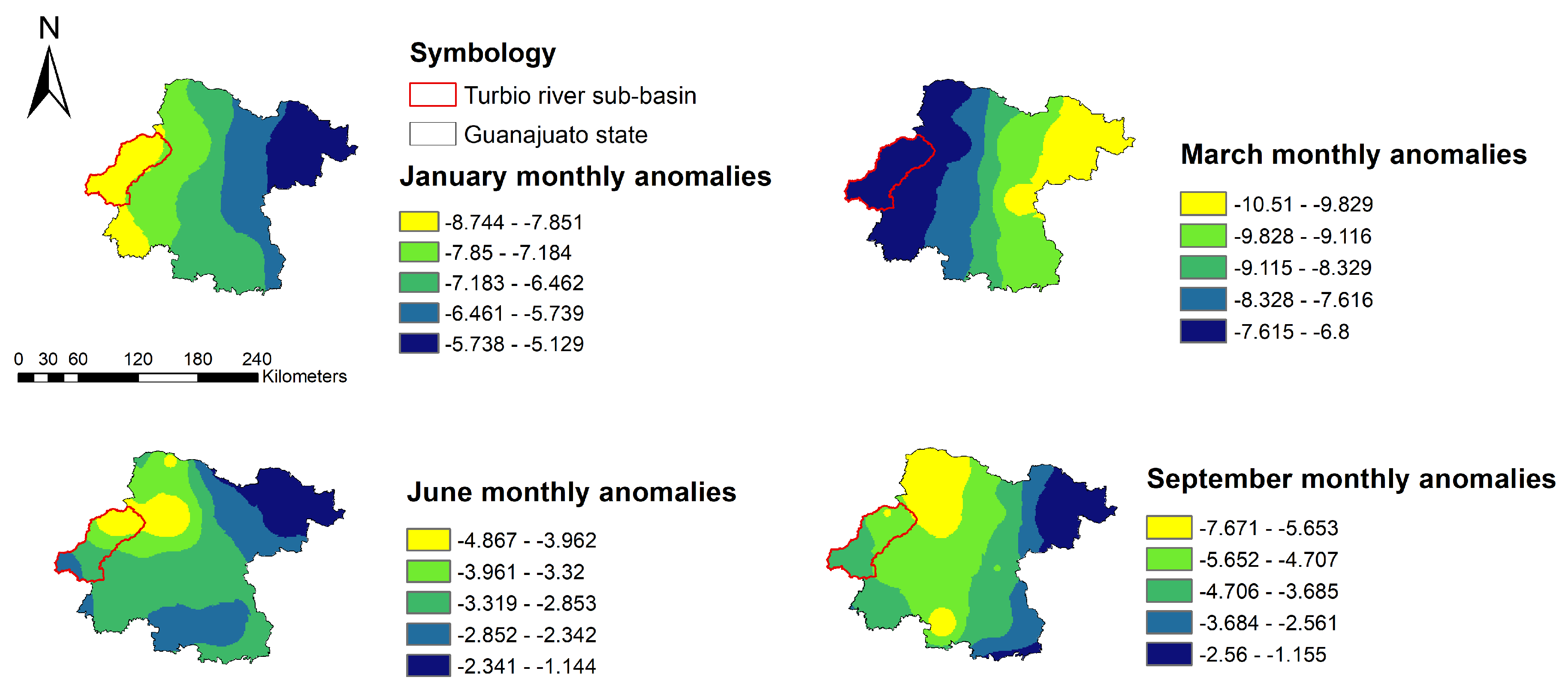
One of the problems of the GCMs is that they have a very large resolution. To solve this problem, the authors [61] divided Mexico into four regions: Northwest, Northeast, South and Southeast to compare the results of the REA with the data from the Climate Research Unit (CRU) [63]. The CRU database is available on http://www.cru.uea.ac.uk/data. In addition to the downscaling performed by the previous authors, we decided to apply a downscaling to the REA projections for the South region (specifically in the state of Guanajuato, which is the region where our study sub-basin is located). Downscaling has been made by combining statistically observed information for the 1971–2000 period, data from the CRU, REA and RCP4.5, RCP6.0 and RCP8.5 scenarios [64]. The authors [61] obtained correlations between REA and CRU higher than 0.8 for the South region. Moreover, significant reductions in the Mean Absolute Error (MAE ≤ 0.9 mm day) and Root Mean Square Error (RMSE ≤ 1.3 mm day). We obtained for the state of Guanajuato a correlation coefficient of 0.78, MAE ≤ 0.99 mm day and RMSE ≤ 1.5 mm day. Figure 7 presents the examples of maps with monthly anomalies obtained with downscaling for the entire state of Guanajuato. These anomalies are introduced as inputs to the TETIS hydrological model to simulate the effects of climate change.
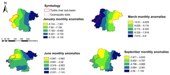
Figure 7.
Examples of monthly precipitation anomalies obtained with downscaling for the RCP4.5 scenario in 2035.
3.4. Forecast of Land Use Changes
For the prediction of future changes in land use and vegetation cover, it has been decided to use the Terrset software [42]. TerrSet is an integrated geospatial software system for monitoring and modeling the earth system for sustainable development. We decided to use Terrset because it uses Markov Chain analysis to project the expected quantity of change and a competitive land allocation model to determine scenarios for a specified future date [65,66]. In addition, the class assignment is based on the contiguity of elements through multicriteria-multiobjective. Its main advantage is that it models with a stronger approach than the other models, since it models the suitability for transition rather than suitability for the ultimate cover class. The technique produced projections maps with an overall accuracy of more than 90% [67]. More information can be found at the link https://clarklabs.org/terrset/land-change-modeler/.
The main input information used in the modeling was the land cover and land use maps at a scale of 1: 250,000, obtained from INEGI. The land use map year 1997 was used in the construction of the Terrset model (Figure 8a), and the VI series (year 2016) was used for the validation of the Terrset model results (Figure 8b).
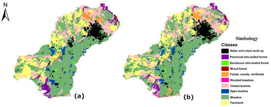
Figure 8.
Land use and vegetation cover maps used in the modeling of future scenarios: (a) year 1997 and (b) series VI.
4. Results and Discussion
4.1. Hydrology Model Performance
The TETIS model adequately reproduces the flows observed at Las Adjuntas gauge for the periods used in calibration (from October 2012 to September 2014) and validation (from October 2005 to September 2008). We decided to use only two hydrological years in the calibration, because there is little information and since according to [68] there is no direct relationship between the number of years and the results of the models. Moreover, that computing times are significantly reduced. Consequently, in the selection of the calibration event, it was necessary to have a wet and a dry year to obtain robust parameters. In terms of efficiency, the model has achieved an average NSE of 0.67, thus, simulating a wet year and a dry year (Figure 9). Calibration is acceptable considering that according to [69], the value of NSE are considered acceptable if it is greater than 0.6 and excellent if it is greater than 0.8. Table 2 shows the average effective parameters obtained by automatic calibration with the SCE-UA algorithm. SMITH2013300.

Figure 9.
Efficiencies of hydrological modeling with TETIS in the calibration period: (a) wet year and (b) dry year (—Qobs = measure discharge and •Qsim = simulated discharge).
Table 3 shows the average effective parameters obtained by automatic calibration with the SCE-UA algorithm, calibrated by correction factors (FC), which make a global correction of the initial parameters quantified with the information available [53].

Table 3.
Average effective parameters obtained by automatic calibration with the Shuffled Complex Evolution (SCE-UA) algorithm.
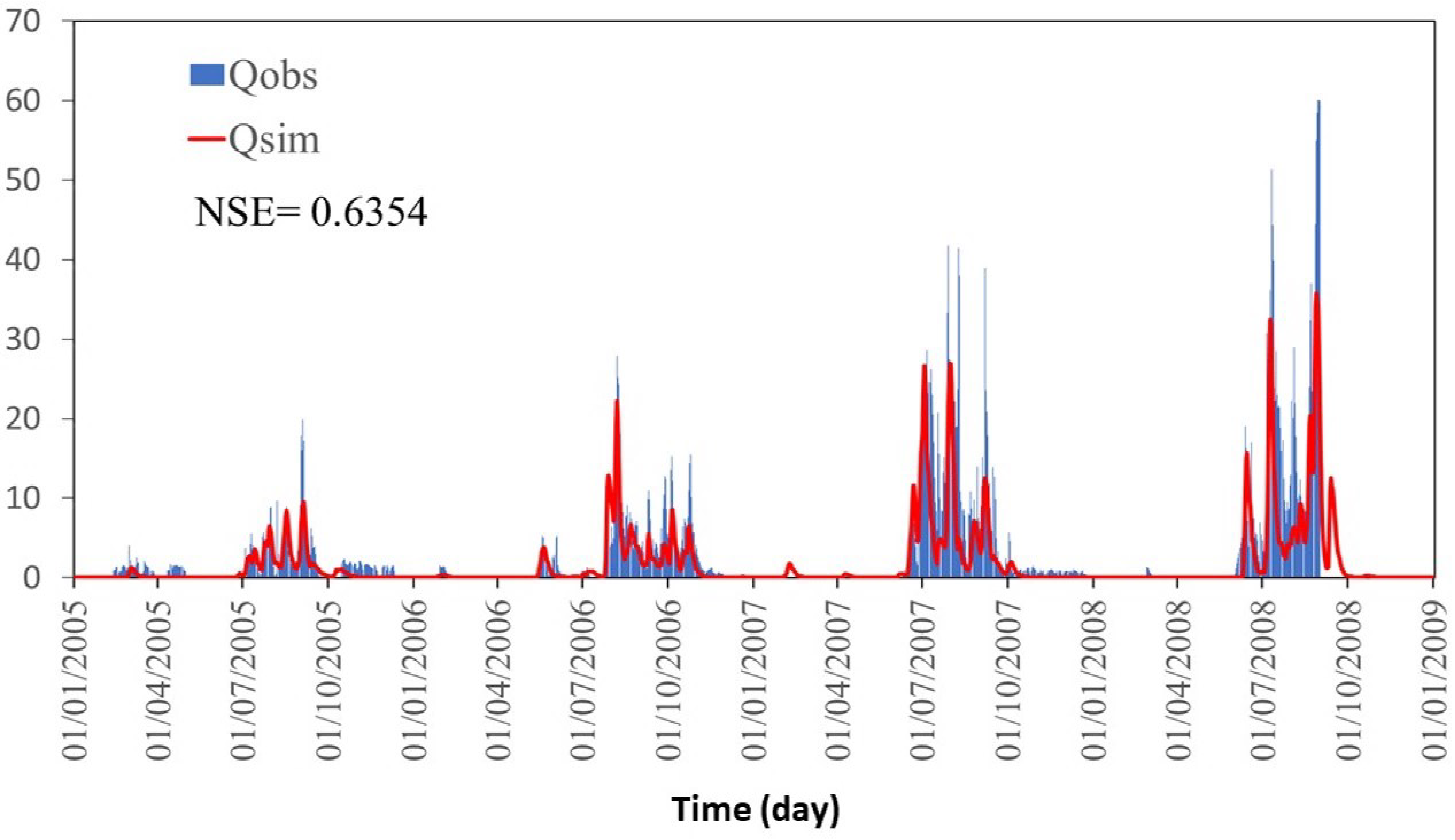
The performance of the model in temporary validation, once again, shows an acceptable behavior of the TETIS model, with an NSE of 0.63 (Figure 10). The NSE obtained in validation shows an acceptable capacity of the model to reproduce the flows in another period, which is different from the one used in the calibration. According to [69], validation is usually considered acceptable if NSE > 0.5 and very good if NSE > 0.7.

Figure 10.
Efficiencies of hydrological modeling with TETIS in the validation period (—Qobs = measure discharge and •Qsim = simulated discharge).
4.2. Climate Projections and Downscaling
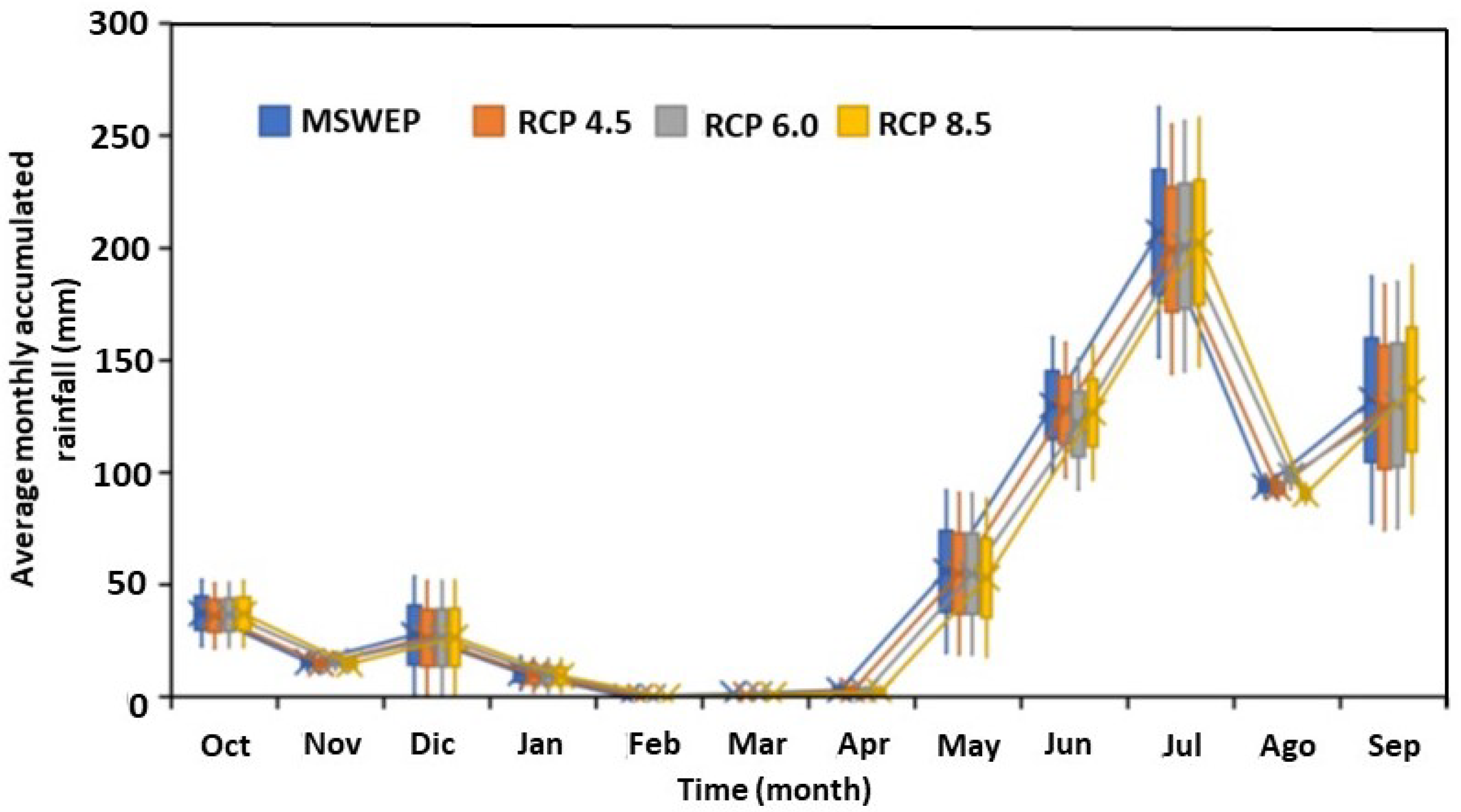
When downscaling the results obtained by the GCM of CMIP5, it was possible to observe a significant reduction in precipitations of the year 2035 for the three scenarios of IPCC (Figure 11). The foregoing depends on the control period used in the comparison. This control period has been generated with historical precipitation data from the MSWEP (period: 1982 to 2014). We have obtained that the REA-CMIP5 models predict an average decrease in rainfall of 1 mm day for the IPCC scenarios. The greatest differences between future projections are presented in the months of the rainy season. The high variability observed in Figure 11 corresponds to the uncertainty calculated for the three scenarios, which is ±2 mm day. We find the same trend in evaluating annual projections (Table 4). The same pattern was observed with annual anomalies, which predict an average decrease in rainfall of 34.7 mm year. The results in Table 4 show that in the near future, the RCP4.5 scenario represents the most critical conditions with a greater decrease in rainfall. However, the projections of REA-CMIP5 in the year 2100 show that RCP8.5 is the most critical with an average decrease in rainfall of 80 mm year (period: 2075–2100).

Figure 11.
Comparison of the control period and the projected rainfall with monthly anomaly maps in the near future (year of 2035).

Table 4.
Average annual rainfall projected with monthly anomalies and their decrease with respect to the control period.
The projections show a general increase in maximum temperatures of up to 2 °C (Table 5). This will have a direct effect on the process of evaporation, evapotranspiration, and consequently, on hydrological availability. The estimated uncertainty for these projections is around ±1 °C for the three IPCC scenarios. The above uncertainty coincides with the results obtained by [61] for the South region of the country. As expected, the most critical scenario for the near future has been RCP8.5. Finally, the REA-CMIP5 project for the year 2100 and the same scenario an increase in temperatures of 4.1 °C.

Table 5.
Increases in the maximum temperatures, obtained with REA-CMIP5 for the IPCC scenarios.
4.3. Future Land Use Change Scenarios Modeling
The validation of land use change projections up to the year 2035 presents 85% of successes, when comparing the vegetation cover of the VI series (Figure 7) and the Terrset results. Once the model was validated, the land use change scenario was generated for the year 2035 (Figure 12). In the projection, it can be observed that the greater changes are seen in the crop land class (Figure 12). Likewise, a significant increase is observed in the urban nuclei. The authors decided not to include the distant future (year 2095) in the research, because we observed inconsistencies in the Terrset prognosis when we distanced from the validation period. In the year 2095, Terrset predicts a decrease in urban areas of 30% compared to 2035 and the occupation of this area by irrigation agriculture, which is not logical considering patterns of large cities growth trend over the last years.
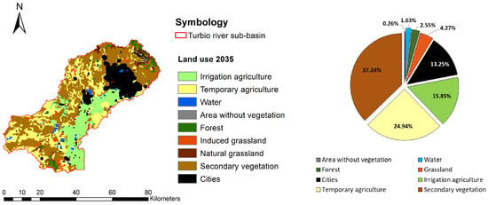
Figure 12.
Projection in Terrset of land use changes for the near future (2035 year).
4.4. Assessment of Vulnerability
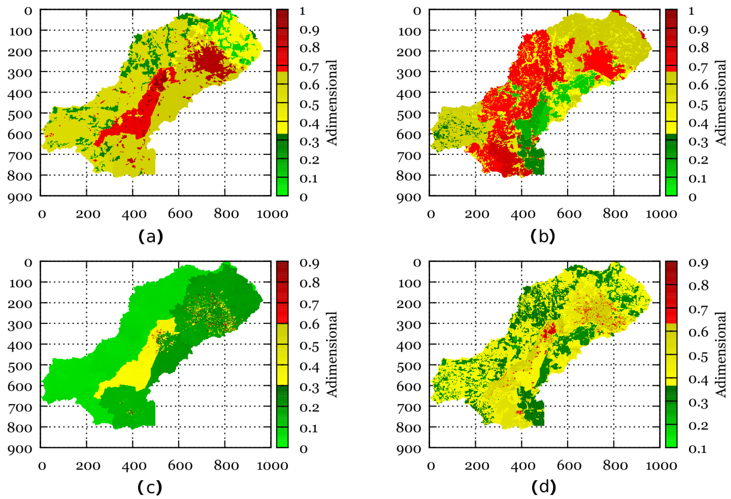
The results obtained with the proposed methodology and the developed MPDV1.0 show that the Turbio river sub-basin presents high vulnerability for the current conditions (Figure 13). The greatest vulnerabilities have been obtained in urban centers and agricultural areas. This coincides with what has been reported in some studies, such as: [70,71]. We decided to analyze more exhaustively the results of hydrological modeling, and observed that infiltration and percolation processes were reduced to 34.5% and 50%, respectively, in urban areas. In addition, 83% of groundwater was extracted in urban centers and urban areas. All this enables us to conclude that the planning and management of the current hydrological availability is not as equitable and sustainable as it was expected. The previous results may change in the cells located in the valley of the Turbio river sub-basin, since in these cells the MSWEP overestimates rainfall by 0.88 mm day. That is to say, the overestimations of rainfall are diminishing the effect of groundwater withdrawals in the formulations of the indicators involved, possibly reducing the vulnerabilities in the cells of the valley of the sub-basin.
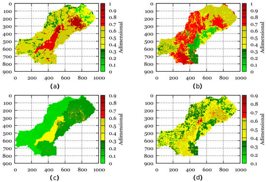
Figure 13.
Vulnerability rate maps obtained with the MPDV1.0 for the current conditions of the Turbio river sub-basin (vulnerability: (a) Environmental, (b) Economic, (c) Social and (d) Global).
The MPDV1.0 forecasts for the near future a generalized increase in vulnerabilities to the potential impacts of climate change and future land use changes (Figure 14 and Figure 15). We expected this increase due to the decrease in rainfall (from 4.97% to 12.32%), predicted by the CMIP5 GCM. There is a potential effect of climate change on evapotranspiration processes, infiltration and percolation. Other authors have also detected these effects for other areas of the world (e.g., [72,73]).
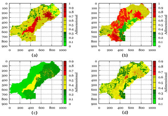
Figure 14.
Maps of vulnerability rates predicted with MPDV1.0 for the year 2035 and scenario RCP8.5 (vulnerability: (a) Environmental, (b) Economic, (c) Social and (d) Global).
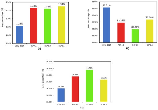
Figure 15.
Global vulnerability occupation area (2035 year): (a) high (), (b) medium () and (c) low ().
By analyzing the vulnerability for each IPCC scenario, we can observe patterns influenced by the characteristics of the scenarios. In general, the greatest vulnerabilities are presented in the RCP6.0 and RCP8.5 scenarios, which surpasses the rest of the scenarios with 0.1% in the sub-basin area and with vulnerabilities of more than 0.5. We believe that the reason for this small increase is because by definition the most drastic scenarios in 2035 have a gradual rise in effects. Likewise, the increase in the use of urban centers and agricultural zones directly influences on the increase of these vulnerabilities. Another interesting conclusion is that according to the hydrological vulnerability rate, the worst conditions for the system are expected in water availability. In other words, practically 75% of the system area will be very vulnerable, with the possibility of not being able to meet the demands of different consumptive uses. The above results are giving indications that there is an urgent need for a restructuring of the management policies that are currently being implemented.
5. Conclusions
In this research, we assess the global vulnerability through hydrological, environmental, economic and social vulnerabilities, taking into consideration the potential impacts of climate change and land use change. In order to achieve this, a new methodology was designed and a Predictive Vulnerability Interface was developed. The results obtained in the study sub-basin show that under current conditions the system is already vulnerable. In the sub-basin, environmental and economic vulnerability is the most important. The areas with the greatest environmental vulnerability were urban centers and agricultural areas, as these areas are where the greatest water vulnerability occurs. This makes evident a restructuring of the management policies that are currently being implemented in the country. In the near future, the situation shows small changes influenced more by the change in land use than by the effects of climate change. The foregoing may be due to the fact that the same degree of exploitation of the sub-basin and the groundwater of the current conditions is considered. This is a non-conclusive result, which will need improvement and further testing. Furthermore, it is necessary to evaluate the uncertainty to detect and improve the variables that introduce the errors in the model. However, if an effect is observed in the sub-basin for each IPCC scenario. This is due to the fact that the Global Climate Models predict a decrease in rainfall and a significant increase in temperature. By integrating these effects of climate and land use changes into the Vulnerability Predictive Interface, there are the combined effects in the flow regimes, producing negative impacts on water resources; thus, a decrease in water availability in the aquifer is predicted. This gives evidence of the great importance of having a methodology such as the one proposed for planning and managing current and future water availability for the region.
Author Contributions
Conceptualization, I.O.; methodology, I.O. and A.M.; software, A.M. and I.O.; validation, I.O., A.M. and V.O.; formal analysis, I.O., A.M. and V.O.; investigation, I.O. and A.M.; resources, I.O. and V.O.; data curation, I.O., A.M. and V.O.; writing—original draft preparation, I.O.; writing—review and editing, I.O.; visualization, I.O., A.M. and V.O.; supervision, I.O.; project administration, I.O.; funding acquisition, V.O. and I.O. All authors have read and agreed to the published version of the manuscript.
Funding
This research received no external funding.
Acknowledgments
The authors thank the Directorate of the Engineering Division, the Directorate of Research and Postgraduate Support and the Rectorate of the Guanajuato Campus of the University of Guanajuato, for the funding granted for the publication of this article.
Conflicts of Interest
The authors declare no conflict of interest.
References
- Füssel, H.M.; Klein, R.J.T. Climate Change Vulnerability Assessments: An Evolution of Conceptual Thinking. Clim. Chang. 2006, 75, 301–329. [Google Scholar] [CrossRef]
- Parry, M.; Canziani, O.; Palutikof, J.; van der Linden, P.; Hanson, C. Climate Change 2007: Impacts, Adaptation and Vulnerability; Cambridge University Press: Cambridge, UK, 2007. [Google Scholar]
- Hinkel, J. “Indicators of vulnerability and adaptive capacity”: Towards a clarification of the science—Policy interface. Glob. Environ. Chang. 2011, 21, 198–208. [Google Scholar] [CrossRef]
- Marsden, T.; Moragues Faus, A.; Sonnino, R. Reproducing vulnerabilities in agri-food systems: Tracing the links between governance, financialization, and vulnerability in Europe post 2007–2008. J. Agrar. Chang. 2019, 19, 82–100. [Google Scholar] [CrossRef]
- Neset, T.S.; Wiréhn, L.; Opach, T.; Glaas, E.; Linnér, B.O. Evaluation of indicators for agricultural vulnerability to climate change: The case of Swedish agriculture. Ecol. Indic. 2019, 105, 571–580. [Google Scholar] [CrossRef]
- Sujakhu, N.M.; Ranjitkar, S.; He, J.; Schmidt-Vogt, D.; Su, Y.; Xu, J. Assessing the Livelihood Vulnerability of Rural Indigenous Households to Climate Changes in Central Nepal, Himalaya. Sustainability 2019, 11, 2977. [Google Scholar] [CrossRef]
- Bakkensen, L.A.; Fox-Lent, C.; Read, L.K.; Linkov, I. Validating Resilience and Vulnerability Indices in the Context of Natural Disasters. Risk Anal. 2017, 37, 982–1004. [Google Scholar] [CrossRef] [PubMed]
- Tung, C.P.; Tsao, J.H.; Tien, Y.C.; Lin, C.Y.; Jhong, B.C. Development of a Novel Climate Adaptation Algorithm for Climate Risk Assessment. Water 2019, 11, 497. [Google Scholar] [CrossRef]
- Li, L.; Cao, R.; Wei, K.; Wang, W.; Chen, L. Adapting climate change challenge: A new vulnerability assessment framework from the global perspective. J. Clean. Prod. 2019, 217, 216–224. [Google Scholar] [CrossRef]
- Gupta, A.K.; Negi, M.; Nandy, S.; Alatalo, J.M.; Singh, V.; Pandey, R. Assessing the vulnerability of socio-environmental systems to climate change along an altitude gradient in the Indian Himalayas. Ecol. Indic. 2019, 106, 105512. [Google Scholar] [CrossRef]
- Ahsan, M.N.; Warner, J. The socioeconomic vulnerability index: A pragmatic approach for assessing climate change led risks—A case study in the south-western coastal Bangladesh. Int. J. Disaster Risk Reduct. 2014, 8, 32–49. [Google Scholar] [CrossRef]
- Koutroulis, A.; Papadimitriou, L.; Grillakis, M.; Tsanis, I.; Warren, R.; Betts, R. Global water availability under high-end climate change: A vulnerability based assessment. Glob. Planet. Chang. 2019, 175, 52–63. [Google Scholar] [CrossRef]
- Ghimire, S.; Dhungana, N.; Upadhaya, S. Impacts of Climate Change on Water Availability and Reservoir Based Hydropower. J. For. Nat. Resour. Manag. 2019, 1, 52–68. [Google Scholar] [CrossRef]
- Tulbure, M.G.; Broich, M. Spatiotemporal patterns and effects of climate and land use on surface water extent dynamics in a dryland region with three decades of Landsat satellite data. Sci. Total Environ. 2019, 658, 1574–1585. [Google Scholar] [CrossRef] [PubMed]
- Jun, K.S.; Chung, E.S.; Sung, J.Y.; Lee, K.S. Development of spatial water resources vulnerability index considering climate change impacts. Sci. Total Environ. 2011, 409, 5228–5242. [Google Scholar] [CrossRef] [PubMed]
- Hewitson, B.C.; Crane, R.G. Consensus between GCM climate change projections with empirical downscaling: Precipitation downscaling over South Africa. Int. J. Climatol. 2006, 26, 1315–1337. [Google Scholar] [CrossRef]
- Chung, E.S.; Park, K.; Lee, K.S. The relative impacts of climate change and urbanization on the hydrological response of a Korean urban watershed. Hydrol. Process. 2011, 25, 544–560. [Google Scholar] [CrossRef]
- Herrera-Pantoja, M.; Hiscock, K. Projected impacts of climate change on water availability indicators in a semi-arid region of central Mexico. Environ. Sci. Policy 2015, 54, 81–89. [Google Scholar] [CrossRef]
- Wiréhn, L.; Danielsson, Å.; Neset, T.S.S. Assessment of composite index methods for agricultural vulnerability to climate change. J. Environ. Manag. 2015, 156, 70–80. [Google Scholar] [CrossRef]
- Boy-Roura, M.; Nolan, B.T.; Menció, A.; Mas-Pla, J. Regression model for aquifer vulnerability assessment of nitrate pollution in the Osona region (NE Spain). J. Hydrol. 2013, 505, 150–162. [Google Scholar] [CrossRef]
- Abson, D.J.; Dougill, A.J.; Stringer, L.C. Using Principal Component Analysis for information-rich socio-ecological vulnerability mapping in Southern Africa. Appl. Geogr. 2012, 35, 515–524. [Google Scholar] [CrossRef]
- Maiolo, M.; Martirano, G.; Morrone, P.; Pantusa, D. Assessment criteria for a sustainable management of the water resources. Water Pract. Technol. 2006, 1, wpt2006012. [Google Scholar] [CrossRef]
- Tixier, J.; Dandrieux, A.; Dusserre, G.; Bubbico, R.; Mazzarotta, B.; Silvetti, B.; Hubert, E.; Rodrigues, N.; Salvi, O. Environmental vulnerability assessment in the vicinity of an industrial site in the frame of ARAMIS European project. J. Hazard. Mater. 2006, 130, 251–264. [Google Scholar] [CrossRef]
- Lange, H.D.; Sala, S.; Vighi, M.; Faber, J. Ecological vulnerability in risk assessment—A review and perspectives. Sci. Total Environ. 2010, 408, 3871–3879. [Google Scholar] [CrossRef] [PubMed]
- Brody, S.D.; Zahran, S.; Vedlitz, A.; Grover, H. Examining the Relationship Between Physical Vulnerability and Public Perceptions of Global Climate Change in the United States. Environ. Behav. 2008, 40, 72–95. [Google Scholar] [CrossRef]
- Armaş, I.; Gavriş, A. Social vulnerability assessment using spatial multi-criteria analysis (SEVI model) and the Social Vulnerability Index (SoVI model)—A case study for Bucharest, Romania. Nat. Hazards Earth Syst. Sci. 2013, 13, 1481–1499. [Google Scholar] [CrossRef]
- Cheng, J.; Tao, J. Fuzzy Comprehensive Evaluation of Drought Vulnerability Based on the Analytic Hierarchy Process: —An Empirical Study from Xiaogan City in Hubei Province. Agric. Agric. Sci. Procedia 2010, 1, 126–135. [Google Scholar] [CrossRef]
- Manning, L.J.; Hall, J.W.; Fowler, H.J.; Kilsby, C.G.; Tebaldi, C. Using probabilistic climate change information from a multimodel ensemble for water resources assessment. Water Resour. Res. 2009, 45. [Google Scholar] [CrossRef]
- Dixon, B. Applicability of neuro-fuzzy techniques in predicting ground-water vulnerability: A GIS-based sensitivity analysis. J. Hydrol. 2005, 309, 17–38. [Google Scholar] [CrossRef]
- Tang, Z.; Engel, B.; Pijanowski, B.; Lim, K. Forecasting land use change and its environmental impact at a watershed scale. J. Environ. Manag. 2005, 76, 35–45. [Google Scholar] [CrossRef]
- Bai, Y.; Ochuodho, T.O.; Yang, J. Impact of land use and climate change on water-related ecosystem services in Kentucky, USA. Ecol. Indic. 2019, 102, 51–64. [Google Scholar] [CrossRef]
- Quintas-Soriano, C.; Castro, A.J.; Castro, H.; García-Llorente, M. Impacts of land use change on ecosystem services and implications for human well-being in Spanish drylands. Land Use Policy 2016, 54, 534–548. [Google Scholar] [CrossRef]
- Chuai, X.; Huang, X.; Wu, C.; Li, J.; Lu, Q.; Qi, X.; Zhang, M.; Zuo, T.; Lu, J. Land use and ecosystems services value changes and ecological land management in coastal Jiangsu, China. Habitat Int. 2016, 57, 164–174. [Google Scholar] [CrossRef]
- Ruiz-Pérez, G.; González-Sanchis, M.; Campo, A.D.; Francés, F. Can a parsimonious model implemented with satellite data be used for modelling the vegetation dynamics and water cycle in water-controlled environments? Ecol. Model. 2016, 324, 45–53. [Google Scholar] [CrossRef]
- Orozco, I.; Francés, F.; Mora, J. Parsimonious Modeling of Snow Accumulation and Snowmelt Processes in High Mountain Basins. Water 2019, 11, 1288. [Google Scholar] [CrossRef]
- Fazeli Farsani, I.; Farzaneh, M.R.; Besalatpour, A.A.; Salehi, M.H.; Faramarzi, M. Assessment of the impact of climate change on spatiotemporal variability of blue and green water resources under CMIP3 and CMIP5 models in a highly mountainous watershed. Theor. Appl. Climatol. 2019, 136, 169–184. [Google Scholar] [CrossRef]
- Harrison, P.A.; Dunford, R.W.; Holman, I.P.; Cojocaru, G.; Madsen, M.S.; Chen, P.Y.; Pedde, S.; Sandars, D. Differences between low-end and high-end climate change impacts in Europe across multiple sectors. Reg. Environ. Chang. 2019, 19, 695–709. [Google Scholar] [CrossRef]
- Wilson, K.; Newton, A.; Echeverría, C.; Weston, C.; Burgman, M. A vulnerability analysis of the temperate forests of south central Chile. Biol. Conserv. 2005, 122, 9–21. [Google Scholar] [CrossRef]
- Wang, X.; Zhong, X.; Liu, S.; Liu, J.; Wang, Z.; Li, M. Regional assessment of environmental vulnerability in the Tibetan Plateau: Development and application of a new method. J. Arid Environ. 2008, 72, 1929–1939. [Google Scholar] [CrossRef]
- Enea, M.; Salemi, G. Fuzzy approach to the environmental impact evaluation. Ecol. Model. 2001, 136, 131–147. [Google Scholar] [CrossRef]
- Nandy, S.; Singh, C.; Das, K.; Kingma, N.; Kushwaha, S. Environmental vulnerability assessment of eco-development zone of Great Himalayan National Park, Himachal Pradesh, India. Ecol. Indic. 2015, 57, 182–195. [Google Scholar] [CrossRef]
- Altuwaijri, H.A.; Alotaibi, M.H.; Almudlaj, A.M.; Almalki, F.M. Predicting urban growth of Arriyadh city, capital of the Kingdom of Saudi Arabia, using Markov cellular automata in TerrSet geospatial system. Arab. J. Geosci. 2019, 12, 135. [Google Scholar] [CrossRef]
- Managing the Risks of Extreme Events and Disasters to Advance Climate Change Adaptation: Special Report of the Intergovernmental Panel on Climate Change; Cambridge University Press: Cambridge, UK, 2012. [CrossRef]
- Ortega-Gaucin, D.; Bartolón, J.; Castellano, H. Water and Climate Change-Danger, Vulnerability and Risk from Droughts in the Context of Climate Change in Mexico; 2018; pp. 78–101. Available online: https://www.gob.mx/imta/documentos/agua-y-cambio-climatico?idiom=es (accessed on 9 June 2020).
- Beck, H.; Van Dijk, A.; Levizzani, V.; Schellekens, J.; Gonzalez Miralles, D.; Martens, B.; de Roo, A. MSWEP: 3-hourly 0.25° global gridded precipitation (1979–2015) by merging gauge, satellite, and reanalysis data. Hydrol. Earth Syst. Sci. Discuss. 2017, 2, 589–615. [Google Scholar] [CrossRef]
- Alijanian, M.; Rakhshandehroo, G.R.; Mishra, A.K.; Dehghani, M. Evaluation of satellite rainfall climatology using CMORPH, PERSIANN-CDR, PERSIANN, TRMM, MSWEP over Iran. Int. J. Climatol. 2017, 37, 4896–4914. [Google Scholar] [CrossRef]
- Beck, H.E.; Wood, E.F.; Pan, M.; Fisher, C.K.; Miralles, D.G.; van Dijk, A.I.J.M.; McVicar, T.R.; Adler, R.F. MSWEP V2 Global 3-Hourly 0.1° Precipitation: Methodology and Quantitative Assessment. Bull. Am. Meteorol. Soc. 2019, 100, 473–500. [Google Scholar] [CrossRef]
- Prakash, S. Performance assessment of CHIRPS, MSWEP, SM2RAIN-CCI, and TMPA precipitation products across India. J. Hydrol. 2019, 571, 50–59. [Google Scholar] [CrossRef]
- Omranian, E.; Sharif, H.O. Evaluation of the Global Precipitation Measurement (GPM) Satellite Rainfall Products over the Lower Colorado River Basin, Texas. JAWRA J. Am. Water Resour. Assoc. 2018, 54, 882–898. [Google Scholar] [CrossRef]
- Dinku, T.; Chidzambwa, S.; Ceccato, P.; Connor, S.J.; Ropelewski, C.F. Validation of high-resolution satellite rainfall products over complex terrain. Int. J. Remote Sens. 2008, 29, 4097–4110. [Google Scholar] [CrossRef]
- Sun, R.; Yuan, H.; Liu, X.; Jiang, X. Evaluation of the latest satellite–gauge precipitation products and their hydrologic applications over the Huaihe River basin. J. Hydrol. 2016, 536, 302–319. [Google Scholar] [CrossRef]
- Jiang, S.; Ren, L.; Xu, C.Y.; Yong, B.; Yuan, F.; Liu, Y.; Yang, X.; Zeng, X. Statistical and hydrological evaluation of the latest Integrated Multi-satellitE Retrievals for GPM (IMERG) over a midlatitude humid basin in South China. Atmos. Res. 2018, 214, 418–429. [Google Scholar] [CrossRef]
- Francés, F.; Vélez, J.I.; Vélez, J.J. Split-parameter structure for the automatic calibration of distributed hydrological models. J. Hydrol. 2007, 332, 226–240. [Google Scholar] [CrossRef]
- Duan, Q.; Sorooshian, S.; Gupta, V. Effective and efficient global optimization for conceptual rainfall-runoff models. Water Resour. Res. 1992, 28, 1015–1031. [Google Scholar] [CrossRef]
- García-Romero, L.; Paredes-Arquiola, J.; Solera, A.; Belda, E.; Andreu, J.; Sánchez-Quispe, S.T. Optimization of the Multi-Start Strategy of a Direct-Search Algorithm for the Calibration of Rainfall–Runoff Models for Water-Resource Assessment. Water 2019, 11, 1876. [Google Scholar] [CrossRef]
- Bauwe, A.; Eckhardt, K.U.; Lennartz, B. Predicting dissolved reactive phosphorus in tile-drained catchments using a modified SWAT model. Ecohydrol. Hydrobiol. 2019, 19, 198–209. [Google Scholar] [CrossRef]
- Giorgetta, M.A.; Jungclaus, J.; Reick, C.H.; Legutke, S.; Bader, J.; Böttinger, M.; Brovkin, V.; Crueger, T.; Esch, M.; Fieg, K.; et al. Climate and carbon cycle changes from 1850 to 2100 in MPI-ESM simulations for the Coupled Model Intercomparison Project phase 5. J. Adv. Model. Earth Syst. 2013, 5, 572–597. [Google Scholar] [CrossRef]
- Neelin, J.D.; Langenbrunner, B.; Meyerson, J.E.; Hall, A.; Berg, N. California Winter Precipitation Change under Global Warming in the Coupled Model Intercomparison Project Phase 5 Ensemble. J. Clim. 2013, 26, 6238–6256. [Google Scholar] [CrossRef]
- Kusunoki, S.; Arakawa, O. Are CMIP5 Models Better than CMIP3 Models in Simulating Precipitation over East Asia? J. Clim. 2015, 28, 5601–5621. [Google Scholar] [CrossRef]
- Knutti, R.; Sedláček, J. Robustness and uncertainties in the new CMIP5 climate model projections. Nat. Clim. Chang. 2013, 3, 369–373. [Google Scholar] [CrossRef]
- Cavazos, T.; Salinas, J.; Martínez-López, B.; Colorado, G.; Grau, P.; González, R.; Conde, C.; Quintanar, A.; Sepúlveda, J.; Centeno, R.; et al. Actualización de Escenarios de Cambio Climático Para México Como Parte de los Productos de la Quinta Comunicación Nacional; Informe final del proyecto al INECC; Instituto Nacional de Ecología y Cambio Climático: Mexico, Mexico, 2013; p. 150. [Google Scholar]
- Giorgi, F.; Mearns, L.O. Calculation of Average, Uncertainty Range, and Reliability of Regional Climate Changes from AOGCM Simulations via the “Reliability Ensemble Averaging” (REA) Method. J. Clim. 2002, 15, 1141–1158. [Google Scholar] [CrossRef]
- Harris, I.; Jones, P.; Osborn, T.; Lister, D. Updated high-resolution grids of monthly climatic observations – the CRU TS3.10 Dataset. Int. J. Climatol. 2014, 34, 623–642. [Google Scholar] [CrossRef]
- Das, J.; Nanduri, U.V. Assessment and evaluation of potential climate change impact on monsoon flows using machine learning technique over Wainganga River basin, India. Hydrol. Sci. J. 2018, 63, 1020–1046. [Google Scholar] [CrossRef]
- Guan, D.; Li, H.; Inohae, T.; Su, W.; Nagaie, T.; Hokao, K. Modeling urban land use change by the integration of cellular automaton and Markov model. Ecol. Model. 2011, 222, 3761–3772. [Google Scholar] [CrossRef]
- Mas, J.F.; Kolb, M.; Paegelow, M.; Olmedo, M.T.C.; Houet, T. Inductive pattern-based land use/cover change models: A comparison of four software packages. Environ. Model. Softw. 2014, 51, 94–111. [Google Scholar] [CrossRef]
- Halmy, M.W.A.; Gessler, P.E.; Hicke, J.A.; Salem, B.B. Land use/land cover change detection and prediction in the north-western coastal desert of Egypt using Markov-CA. Appl. Geogr. 2015, 63, 101–112. [Google Scholar] [CrossRef]
- Smith, M.; Koren, V.; Zhang, Z.; Moreda, F.; Cui, Z.; Cosgrove, B.; Mizukami, N.; Kitzmiller, D.; Ding, F.; Reed, S.; et al. The distributed model intercomparison project—Phase 2: Experiment design and summary results of the western basin experiments. J. Hydrol. 2013, 507, 300–329. [Google Scholar] [CrossRef]
- Moriasi, D.N.; Arnold, J.G.; Van Liew, M.W.; Bingner, R.L.; Harmel, R.D.; Veith, T.L. Model Evaluation Guidelines for Systematic Quantification of Accuracy in Watershed Simulations. Trans. ASABE 2007, 50, 885–900. [Google Scholar] [CrossRef]
- Freitas, L.; Afonso, M.J.; Pereira, A.J.S.C.; Delerue-Matos, C.; Chaminé, H.I. Assessment of sustainability of groundwater in urban areas (Porto, NW Portugal): A GIS mapping approach to evaluate vulnerability, infiltration and recharge. Environ. Earth Sci. 2019, 78, 140. [Google Scholar] [CrossRef]
- Okadera, T.; Wang, Q.X.; Deni, E.; Nakayama, T. Groundwater monitoring for evaluating the pasture carrying capacity and its vulnerability in arid and semi-arid regions: A case study of urban and mining areas in Mongolia. IOP Conf. Ser. Earth Environ. Sci. 2019, 266, 012013. [Google Scholar] [CrossRef]
- Dinpashoh, Y.; Jahanbakhsh Asl, S.; Rasouli, A.; Singh, V. Impact of climate change on potential evapotranspiration (case study: West and NW of Iran). Theor. Appl. Climatol. 2018, 136, 185–201. [Google Scholar] [CrossRef]
- Doglioni, A.; Simeone, V. Effects of Climatic Changes on Groundwater Availability in a Semi-arid Mediterranean Region. In IAEG/AEG Annual Meeting Proceedings, San Francisco, California, 2018—Volume 4; Shakoor, A., Cato, K., Eds.; Springer International Publishing: Cham, Switzerland, 2019; pp. 105–110. [Google Scholar]
© 2020 by the authors. Licensee MDPI, Basel, Switzerland. This article is an open access article distributed under the terms and conditions of the Creative Commons Attribution (CC BY) license (http://creativecommons.org/licenses/by/4.0/).

