Abstract
Access to a reliable water supply is central for a well-functioning society. However, water supply systems are subject to a wide range of threats which may affect their ability to provide water to society. This paper presents a novel risk assessment approach that enables thorough analyses of economic losses and associated uncertainties under a range of water supply disruption scenarios. The purpose is to avoid sub-optimization when prioritizing between risk reduction measures, by integrating the full range of possible outcomes from low to high probability events. By combining risk analysis with cost-benefit analysis, additional information is provided on measures for leveraging investments in managing and reducing the risks. This enables the identification of the most economically profitable risk reduction alternatives and enables decision makers to build strategic capacity for operating in difficult and uncertain futures. The presented approach is exemplified on the island of Gotland, one of the most water scarce areas of Sweden.
1. Introduction
Water supply infrastructure systems are subject to a wide range of threats which may affect their ability to provide water to society. Predicted population growth and hydro-climatic changes are expected to contribute to both an increased probability of water scarcity and more severe societal consequences [1,2]. In addition to threats related to reduced access to and quality of raw water, failures in water provision may also occur due to events related to the treatment systems, e.g., component failures in treatment plants, and related to the distribution systems, e.g., pipe bursts and pump failures. To deal with the uncertainties and the societal impacts that all these threats entail, risk assessment methods need to be integrated in water supply decision making [3,4]. Risk assessments may be performed in different ways, but a common approach is to qualitatively and/or quantitatively estimate and combine the consequences of one or several possible scenarios, typically undesirable events, the probability of occurrence for the scenarios and the uncertainties related to the included factors [5]. Risk-based decision making uses the results of risk assessments to guide and inform decisions on risk reduction measures. It may, for example, involve comparing required resources for implementing potential risk reduction measures with potential benefits of estimated risk reduction. A framing based on risk provides for a better understanding of the severity, distribution and impacts of the full range of possible outcomes [6].
Decision-makers and water supply managers face difficult decisions on resource allocation and prioritizations of risk reduction measures. To support such decisions, effective risk management requires the identification and assessment of a range of representative risk scenarios [7]. The process of summing and showing the interaction between single or individual risks is sometimes referred to as risk aggregation [8]. Moreover, to facilitate rational decision-making, the risk should be expressed in a clear manner, and related uncertainties considered [9]. In this paper, the focus is on economic consequences, and risk is expressed in terms of economic consequences to society arising from water supply disruption events. A disruption in the water provision can lead to economic consequences for the water utility as well as for businesses and residential consumers, and may generate significant economic losses for society [10]. Several different methods have been used to estimate business interruption losses, e.g., input-output models and computable general equilibrium models [11]. The direct economic consequences to commercial and industrial consumers are often estimated by use of importance (or resiliency) factors, i.e., quantitative measurements focusing on the production output during disruption [12]. Residential welfare loss of water supply disruptions can be assessed based on estimates of consumer willingness to pay to avoid such disruptions [13,14]. Short-term disruption events are not evaluated as frequently as long-term disruptions. They may, however, contribute significantly to the total economic losses due to their much higher frequency [10].
According to Uzielli, et al. [15], a quantitative risk assessment should include a quantification of the expected losses, based on the probability for a given event, the economic consequences to society of exposed elements at risk, and their associated vulnerability. However, risk assessments are often complex in nature, and many aspects of the risk may be subject to large uncertainties [16]. It is now common to define risk using uncertainty as a key factor, see e.g., International Organization for Standardization (ISO) [17] and Aven [18]. The importance of considering uncertainties is particularly true for factors affecting high-impact-low-probability risks which, by their very nature, occur only infrequently. Existing statistics may be insufficient to support the risk assessments [19]. Data samples may, for example, be too small, too unreliable, too costly to obtain, or simply unobtainable. In these cases, the only sound option may be to elicit the information needed using expert judgements. The typical way is to elicit judgement from more than one expert and represent the uncertainties by probability distributions [20,21,22], so that appropriate decisions can be made on risk reduction. The approach proposed in this paper integrates the full range of risk scenarios, while taking the underlying uncertainties into account, to estimate the total risk of the water supply system. This allows for a better understanding of how different factors influence each component of risk and how they, in turn, affect the total risk. It further facilitates a design and prioritization of measures that focus on addressing the total risk rather than individual threats.
The overall aim of this paper is to provide a risk assessment method that enables thorough analyses of risk reduction measures by integrating the full range of possible outcomes from low to high probability events. The purpose of the method is to provide a structured and thorough analysis of the total risk to enable prioritization of possible measures based on, e.g., economic profitability. A key part is also to avoid sub-optimization, where risk reduction measures are prioritized based on individual events. Specific objectives are to: (1) provide a method that enables estimation of economic losses under various levels of water supply disruption events; (2) combine this information with the integrated likelihood function of disruption events to estimate the total risk under existing conditions; (3) analyze and compare the annual benefits and economic profitability of risk reduction measures; and (4) exemplify this method by application on the island of Gotland, Sweden. The proposed approach is a valuable contribution to the water supply reliability literature, in which definition of risk scenarios, uncertainty estimations of input variables, economic valuation of consequences, calculations of the total integral sum of risk over different risk scenarios and calculations of economic profitability through cost benefit analysis (CBA) all are rare.
2. Materials and Methods
In short, the risk assessment method described in this paper is based on a combination of quantitative risk analysis and CBA [23]. The main steps are: (1) identification of risk scenarios; (2) estimation of factors affecting the risk; (3) characterization of risk; (4) evaluation of risk reduction measures; and (5) performance of uncertainty and sensitivity analyses. The methodology is described in more detail in the following paragraphs.
2.1. Identification of Risk Scenarios
In this paper, a well-established approach to risk analysis is used where the aim is to answer the following three questions [9]:
- What can go wrong?
- How likely is it to happen?
- If it does happen, what are the consequences?
To answer these questions, a set of scenarios are defined. The set of scenarios used in a quantitative risk analysis should preferably be complete, finite and disjoint [24]. This means that a nonoverlapping subset of N scenarios together should represent all possible risk scenarios for the entire problem so that the total risk R is
where is scenario i, ; is the frequency with which the scenario occurs; and is the consequence given that scenario i occurs. Furthermore, the uncertainties related to the three variables are identified and described quantitatively or qualitatively to enable a thorough description of the risk.
There are several scenario identification methods used within the theory of scenario structuring (TSS), e.g., hierarchical holographic modeling (HHM), failure modes and effects analysis (FMEA), hazard and operations analysis (HAZOP), and anticipatory failure determination (AFD). All methods start by defining a success scenario. The risk scenarios (si) can then be identified by decomposing the success scenario into different parts, e.g., in geographical, hydrological, temporal or functional parts, and asking; “What can go wrong in this part?” or “What happens if this parameter changes?”. The aggregated risks of all scenarios then determine the total risk of the overall system [24].
2.2. Estimation of Factors Affecting Risk
As mentioned above, the risk is defined as a function of a set of scenarios, the frequency with which they occur and the consequences if they occur. When we do not know the frequencies or the consequences with certainty, we can express them by probability distributions so that , where and are the probability density functions for the frequency and consequence, respectively. In this study, the following economic consequences are considered: residential welfare losses, businesses losses, and water utility expenditures for upholding water provision (as far as possible) during the disruptions. The water utility expenditures were estimated based on information from the local water utility from previous experiences. In the subsections below it is described how uncertain quantities, of e.g., the return periods and duration of events, were estimated based on formal expert elicitation, and how residential welfare losses and business losses were calculated.
2.2.1. Formal Expert Elicitation
One technique of capturing the probability distributions of uncertain quantities is to elicit this information using a range of experts from different disciplines. In this paper, uncertain quantities, such as return period and duration of events, were estimated by expert elicitation using the Sheffield Elicitation Framework (SHELF) [25]. The SHELF framework elicits a single judicious consensus distribution from the expert group for each uncertain quantity. The process begins by eliciting individual judgements from each expert independently, followed by a group discussion and a group judgement. The parameters estimated in this paper were the lower and upper plausible limits for the uncertain quantity, as well as the median and lower and upper quartiles. The MATCH Uncertainty Elicitation Tool [26] was used to find the best fitted statistical distribution model for the group judgment and to provide direct visual feedback to the expert. The results were reviewed and discussed by the group and when necessary adjusted to fit their final and joint preferences.
2.2.2. Estimation of Household Welfare Losses
One consequence of water disruptions is residential welfare losses. In this paper, this was valued based on estimates of consumer willingness to pay to avoid water supply shortages [13,14]. By integrating the demand curve for water, between baseline consumption and reduced consumption, the daily welfare loss for a consumer in region j facing a water shortage of z at time t was calculated as:
where is the average water price when no shortage, is the average amount of water consumed per capita per day when no shortage, is the reduced water consumption, and ƞ is the price elasticity of water demand. The severity of the water shortage was defined as ϵ [0,1], where corresponds to no water and corresponds to normal water availability [13].
The average water price on Gotland in 2017 was 12.74 SEK/m3 (100 Swedish Krona (SEK) ≈ 10 USD in October 2019) and the average amount of water consumed was 132 L per capita and per day [27]. There is no price elasticity estimate available for Gotland. Therefore, a mean price elasticity of water demand for developed countries (−0.378) was applied, based on the meta-analysis by Sebri [28] (p. 518). For sensitivity analysis, a price elasticity of −0.2 was used, following a study of household water demand in Sweden [29]. was estimated at the SHELF workshops.
2.2.3. Estimation of Business Losses
Another consequence following water disruptions is the economic consequences for commercial and industrial customers due to loss of potable water service. In this paper, the estimation of value added lost for businesses followed the Federal Emergency Management Agency (FEMA) [30] (p. 39) methodology of using local GDP data [31] in combination with water importance factors [32]. It was here assumed that Swedish economic sectors have the same percentage reduction in value added from water supply disruptions as US economic sectors.
2.3. Risk Characterization
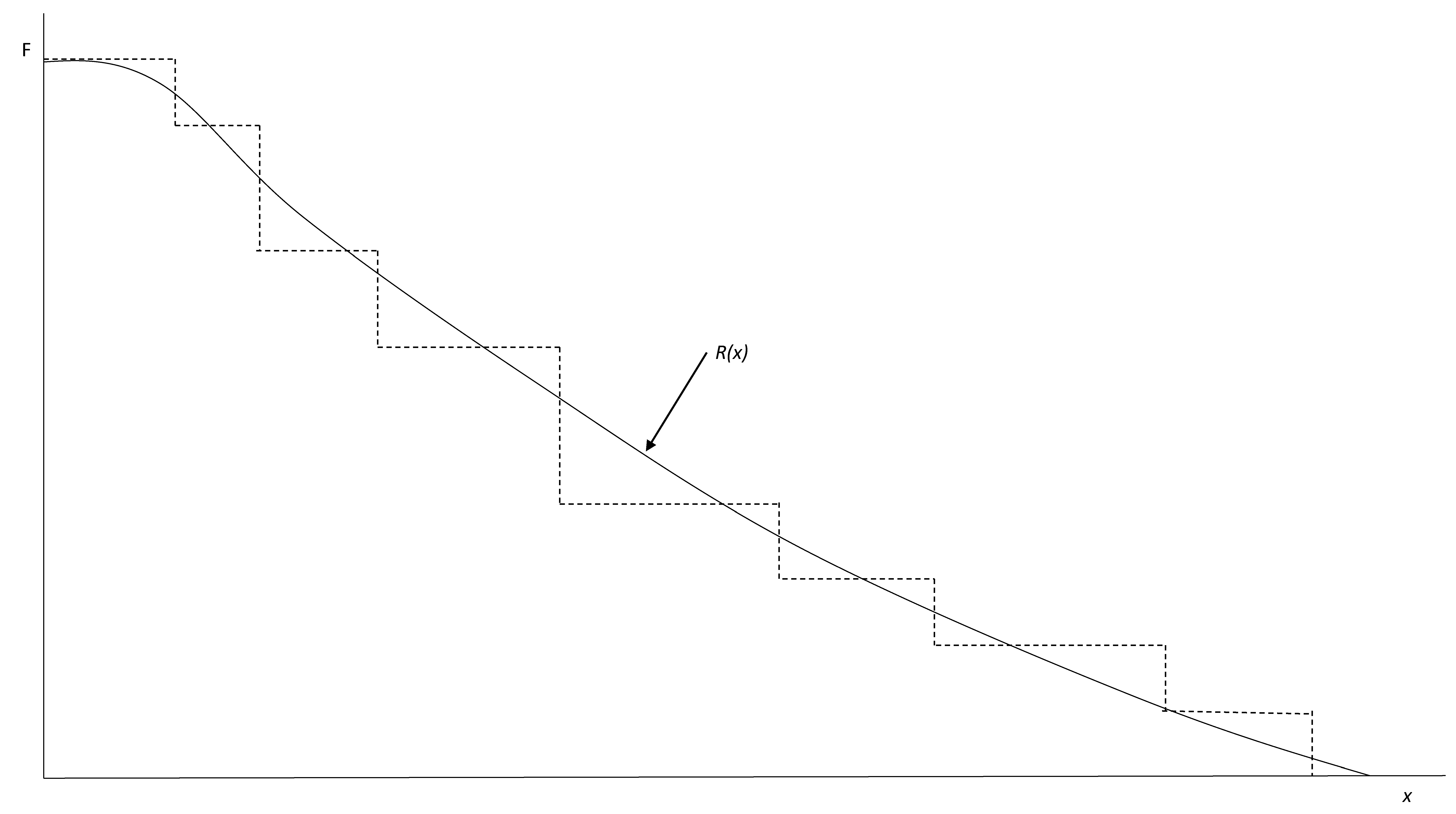
A risk curve for the reference alternative, i.e., the current water supply system, is developed based on the triplets . For this, the scenarios must first be arranged in order of increasing consequences, i.e., , along with corresponding frequencies. Starting with the scenario with the most severe consequences, a cumulative frequency , i.e., the frequency of having consequence equal to or greater than , is calculated as . By plotting , a staircase function of the analyzed risk scenarios is derived, representing a discrete approximation of the continuous reality. A smoothed risk curve , drawn through the staircase (Figure 1), can then be regarded to represent the actual risk [9]. Each point of the curve does not belong to a specific event but instead represents the estimated return period of losses. The integral of the curve, i.e., the area underneath the curve, represents the total expected losses in any given year so that:
where is the total annual risk, N is the total number of analyzed scenarios, x is the combined economic consequences for the municipality, households and businesses (i.e., ), and F is the cumulative frequency as a function of consequence x. For risk estimation, the continuous function is simplified by the staircase function.
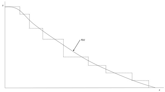
Figure 1.
Schematic description of staircase and continuous risk functions based on e.g., Kaplan and Garrick [9].
2.4. Evaluation of Risk Reduction Measures
A risk reduction measure is here defined as any measure that can be applied to reduce the frequency and/or the consequences of the undesirable events. The same scenarios used when estimating the risk level of the reference alternative are also used to assess potential risk reduction measures, but the measures’ associated frequencies and consequences are applied. For each measure (a), a new risk curve is created and thus a new annual total risk. The annual risk reduction, i.e., the annual benefit , is calculated as the difference between the risk curve of the reference alternative and the risk curve of the analyzed measure as .
To compare the economic profitability of implementing the measures, a CBA [23] was performed. CBA is a structured method to compare the societal costs of an option with its benefits. The estimated risk reductions were included in the CBA as annual benefits [33]. The decision-metric of the CBA is the net present value (NPV), calculated as:
where a is the alternative measure, t is the time when benefit or cost occur, T is the time horizon, r is the discount rate, C are the costs associated with implementing a risk reduction measure, and B is the benefit of risk reduction in relation to the reference alternative. A measure is considered economically profitable when its total benefits to society are larger than its total costs to society, i.e., when its NPV is positive. Three discount rates were used (1.4%, 3.5% and 5%, respectively), reflecting the average discount rate used in the Stern Review on Climate Change [34] and the suggested social and private rates of the Swedish Transportation Administration Guidelines for cost-benefit analysis [35].
2.5. Uncertainty and Sensitivity Analyses
This paper applies a probabilistic approach with formal uncertainty analysis. As described above, the SHELF Framework was used to elicit information regarding uncertain quantities such as the proportion of households affected in different scenarios and the frequency of events. Probability distributions were assigned to represent each uncertain quantity, and Monte Carlo simulations (10,000 iterations) were used to calculate the annualized risks, risk reductions and NPVs using the risk analysis software @Risk 7.6.0 (Palisade, Ithaca, USA). This provides important additional information for the decision-makers. As Kaplan and Garrick [9] (p. 14) state, a single number is not a big enough concept to communicate a risk—it takes a whole family of risk curves. The uncertainties in input data can, for example, be used to visualize the resulting mean, minimum and maximum risk curves. The uncertainties can also be transferred in loss exceedance curves, i.e., the probability that the expected loss exceeds a certain value [36]. Since it is hard, and often not possible, to capture all uncertainties in the variables of a risk model, other uncertainty factors are identified, described and discussed using a qualitative approach. The purpose is to provide a transparent decision support that highlights uncertainties that may affect the interpretation of the results.
3. Method Application
3.1. The Case Study Site
The case study site was the island of Gotland (3000 km2) in Sweden, located in the Baltic Sea about 100 km east of the mainland and with a population of 58,000. Gotland suffers from low water availability and difficulties in providing enough water to the society. The island’s thin soil layers, lack of coherent reservoirs in the limestone bedrock and extensive drainage of arable land, result in an overall low storage capacity of water and a high precipitation run-off [37]. Climate change is expected to further limit the water availability on the island. Longer dry periods are predicted during summers, and the groundwater recharge is expected to decrease due to an increased temperature and the subsequent increase in evaporation and vegetation periods. Currently, about 18 million cubic meter per year is used by households (4 Mm3), animal keeping (1.5 Mm3), tourism (1.3 Mm3), industry (6.1 Mm3) and irrigation (5 Mm3) [38]. A large proportion of the water supply is based on private solutions. For example, only 67% of the households are connected to the public water supply system, which during the summer months to 40% is based on groundwater, 20% on surface water and 40% on desalinated seawater [39].
Gotland is one of the most popular tourist summer destinations in Sweden. In 2016, over 2 million people traveled to Gotland, and the number of guest nights at hotels and other commercial accommodation facilities exceeded 1 million [40]. Hence, there is a large seasonal variation of water demand on the island with the highest demand occurring when the water supplies are at their lowest. In addition to an already constrained water supply situation, the total water demand, i.e., of municipal water provision and other water sources, is expected to increase by about 40% by 2045 with increases of 30% in tourism, 20% in domestic demand, 20% in animal keeping, 15% in industry, and 100% in irrigation [38]. The current water resources on the island cannot meet this projected increase in demand, especially during the summer months. Due to Gotland’s insular location there is also no possibility to strengthen the water supply from neighboring municipalities.
3.2. Scenarios and Risk Reduction Measures
Six scenarios were identified around the question: What can pose a challenge to maintain a continuous municipal water supply provision on Gotland? see Table 1. The scenarios were developed during multiple discussions with the municipality’s water supply strategists to represent the range of possible events that may present challenges to the municipal water supply. More detailed information about the scenarios was discussed at the workshops but is confidential for safety reasons.

Table 1.
Scenario summaries.
Based on previous estimates of where, and with how much, the municipality can increase groundwater and surface water abstractions as well as supplement groundwater catchments by managed aquifer recharge (MAR) [37,41], four alternative risk reduction measures were analyzed in this paper, see Table 2. Focus in this paper is hence on improvements in the raw water system. The analyzed measures are site specific, thus they can reduce the risk in the areas in which they are applied but not in areas to which, e.g., the distribution network is not connected. The reason desalination is not further explored is because the municipality has decided to prioritize freshwater (from groundwater, lakes and streams) over seawater for public water supply. Desalination is to be further considered only if the freshwater resources cannot meet demand [42].

Table 2.
Alternative risk reduction measures.
To estimate uncertain factors affecting identified scenarios and risk reduction measures, three half day SHELF elicitation workshops [25] were held in May and June 2019, with workshop participants ranging from 2 to 6 experts and 1 to 3 workshop facilitators. The workshop participants (6 in total) represented the following areas of expertise: public drinking water management, public water supply strategy, emergency management, environmental expertise, private water supply, and longtime operational water utility staff. For the more frequent events, there was plenty of background information to rely on regarding, e.g., estimation of different cost aspects. For the more infrequent events, the estimations were naturally more speculative.
4. Results
Details on quantified variables from the SHELF workshops and follow up meetings are provided in Table 3. The table provides the input variables for the calculations of total risk, risk reduction and net present values (NPV), performed by Monte Carlo simulations. For a few events that are expected to occur each year, uncertainties regarding frequency and return period were not quantified. Frequency was generally used as a measurement of occurrence when the estimated time between events was greater than one time per year; otherwise the return period was used.

Table 3.
Estimates of input variables. Distributions used are log-normal, LN (μ; σ), beta, B (α1; α2; min; max) and gamma, G (α; β). R0 = reference alternative; GW = groundwater extraction; MAR = managed aquifer recharge; SW small = surface water extraction small scale; SW large = surface water extraction large scale.
The results and related uncertainties are dependent on the estimated input variables but also on the basic assumptions used to describe the system and the future development. Table 4 provides information on non-quantified uncertainty factors discussed at the SHELF workshops, along with the associated assumptions made. This qualitative analysis of uncertainties is of great importance when interpreting the results.

Table 4.
Non-quantified uncertainty factors discussed at the Sheffield Elicitation Framework (SHELF) workshops.
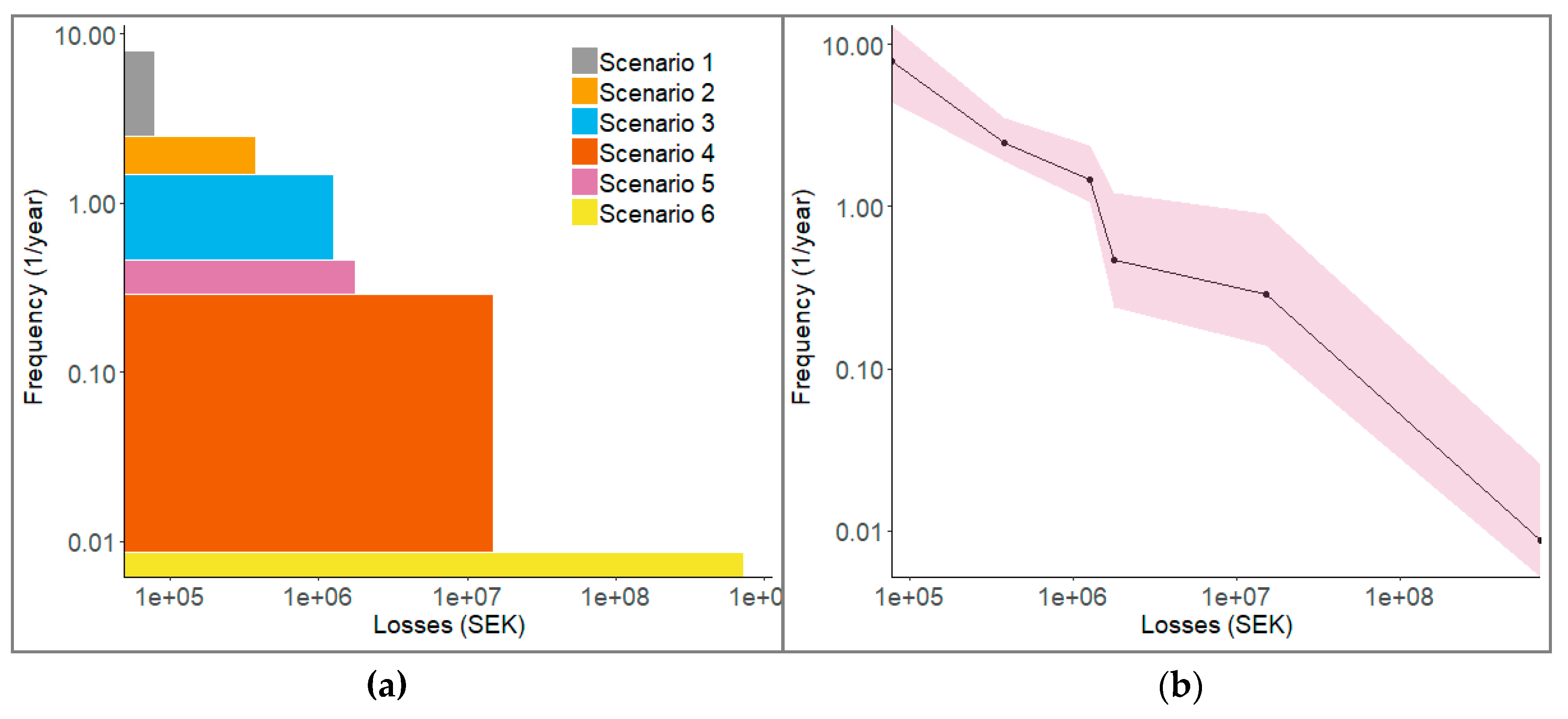
The estimated annual risk for the reference alternative is demonstrated in Figure 2 in the form of a staircase to the left and as a risk curve showing the mean and P05 and P95 frequency percentiles to the right. According to calculation results, the low-frequency events are generally associated with larger economic consequences than high-frequency events. However, the annual risk is the lowest for the second least frequent event (Scenario 5) and the highest for the most frequent event (Scenario 6): 425,000 SEK for Scenario 1; 378,000 SEK for Scenario 2; 1,262,000 SEK for Scenario 3; 4,222,000 SEK for Scenario 4; 309,000 SEK for Scenario 5; and 6,321,000 SEK for Scenario 6 (mean values). The total annual risk is estimated at approximately 12,916,000 SEK, ranging from 7,161,000 SEK to 32,370,000 SEK for the 5th and 95th percentiles, respectively (mean values).
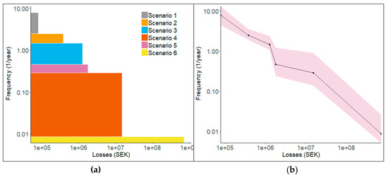
Figure 2.
Estimated annual risk of the reference alternative for analyzed scenarios in the form of staircase (a), and in the form of a risk curve showing the mean values and frequency percentiles P05 and P95 (b). Note that the curves are plotted on log-log scales with cumulative frequencies.
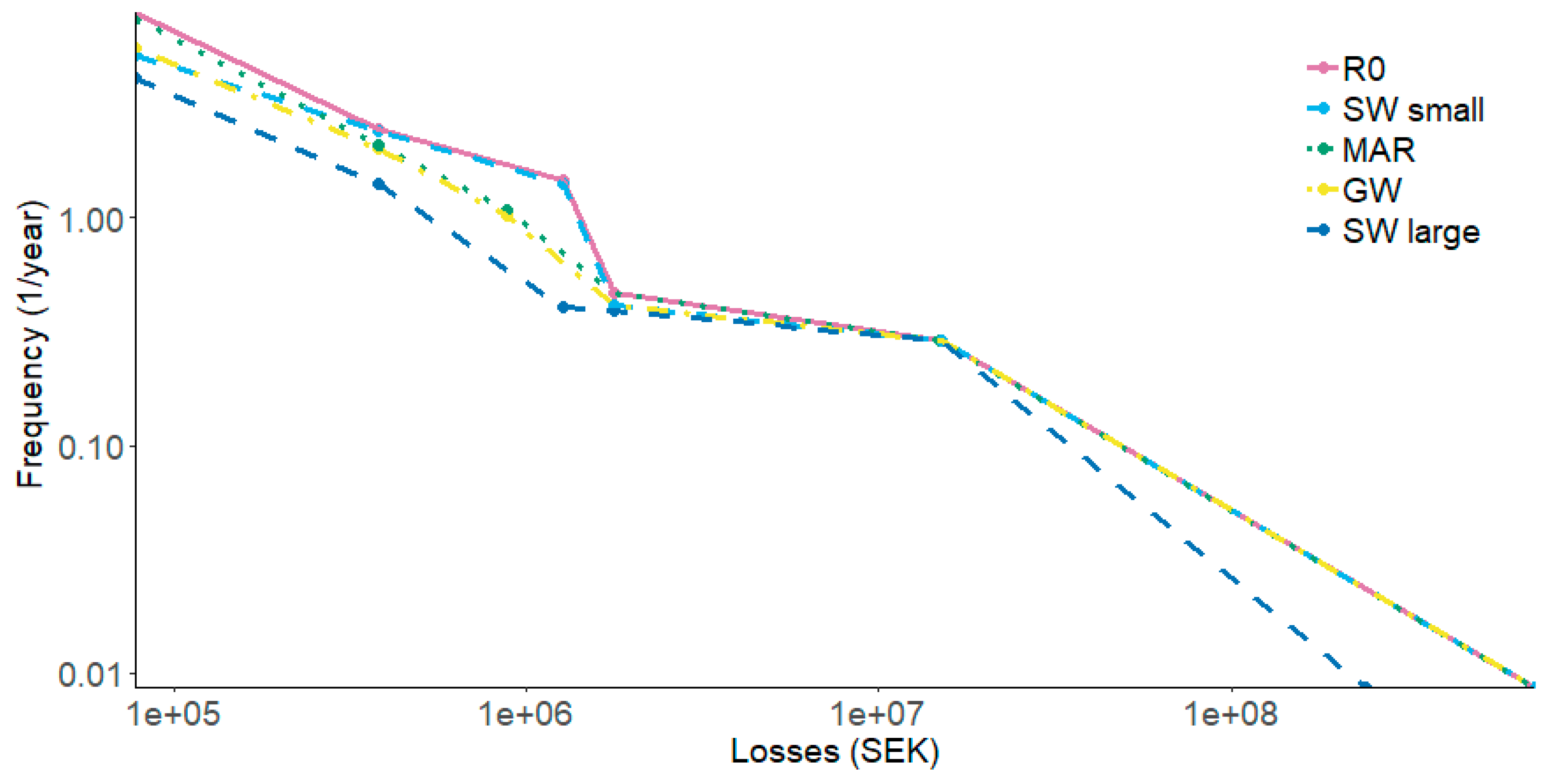
The risk curves of the alternative risk reduction measures are shown in Figure 3 along with the risk curve of the reference alternative. The potential risk reduction of the measures is the difference between the risk curve of the reference alternative and those of the measures. The large-scale surface water measure was shown to reduce the total annual risk the most, suggesting a potential reduction of approximately 6 million SEK annually compared to 965,000 SEK for groundwater, 785,000 SEK for MAR, and 307,000 SEK for the small surface water measure (mean values).
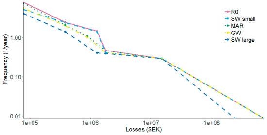
Figure 3.
Risk curves for analyzed risk reduction measures over all scenarios (mean values). Note that the curves are plotted on log-log scale with cumulative frequencies.
The probabilities of each measure being the best option with respect to risk reduction for each individual scenario and combined for all scenarios is shown in Figure 4. The results show that the large-scale surface water measure has the highest probability to be the best option for most individual scenarios and for all scenarios combined. The ranking order of the other measures vary between risk scenarios.
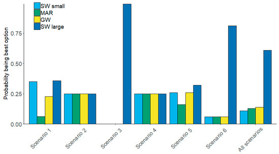
Figure 4.
Probability that each measure is the best option with respect to risk reduction.
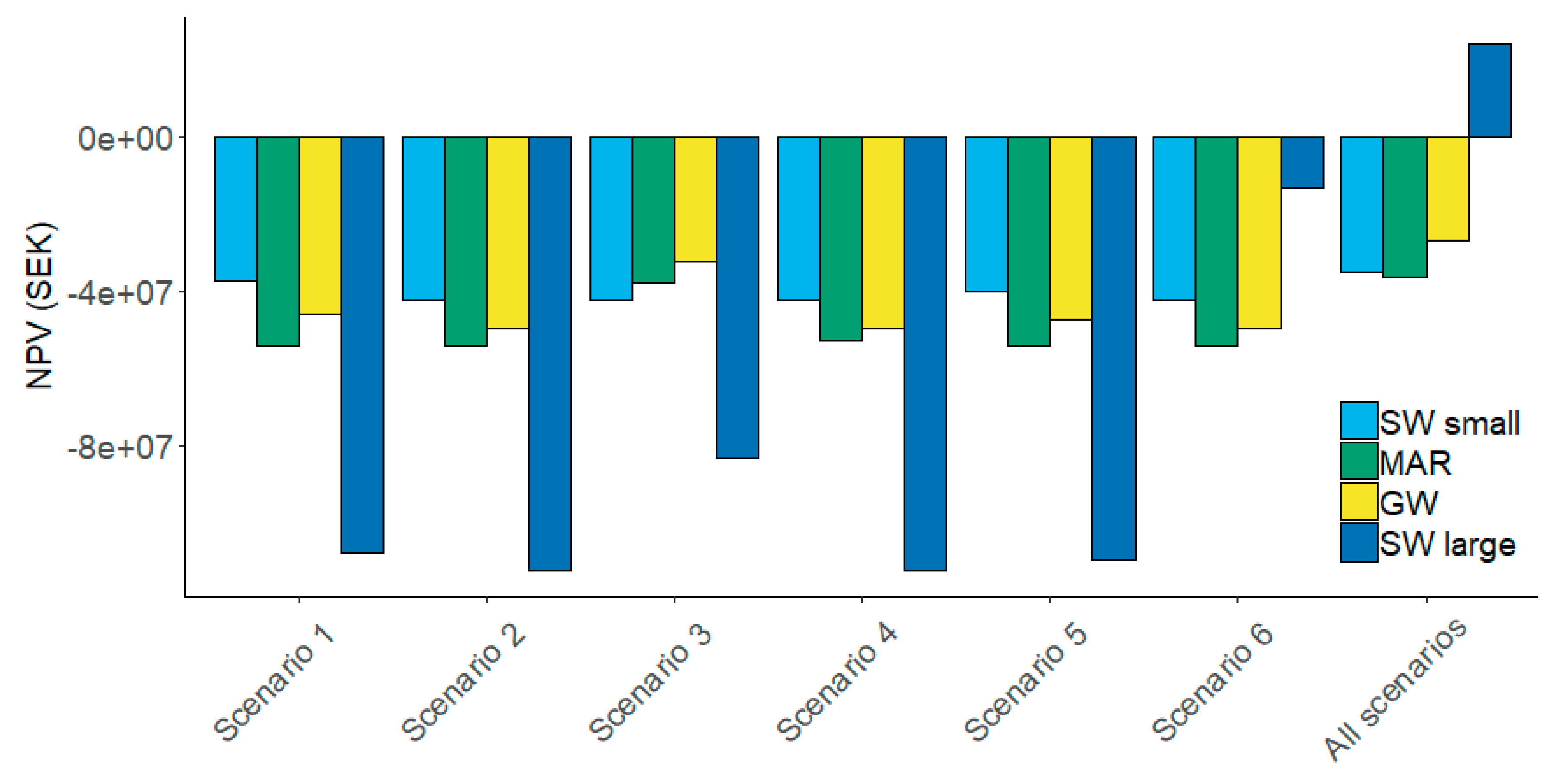
The result from the cost-benefit analysis is shown in Figure 5 displaying that the large-scale surface water measure was the least economically beneficial measure for Scenarios 1 to 5 when analyzed individually, but the most beneficial measure for Scenario 6 and when including the risk reduction for all scenarios combined. The ranking order of the other measures varied somewhat between the analyzed scenarios. The NPV mean values in million SEK for the measures SW small, MAR, GW, and SW large respectively are: −37, −54, −46, and −108 (Scenario 1); −42, −54, −50, and −113 (Scenario 2); −42, −38, −33, and −83 (Scenario 3); −42, −53, −50, and −113 (Scenario 4); −40, −54, −47, and −109 (Scenario 5); −42, −54, −50, and −13 (Scenario 6); and −35, −36 −27 and 24 (all scenarios combined). It is worth noting that the NPVs are based only on implementation costs and the benefits of risk reduction with respect to water supply disruptions. The CBA could therefore be improved by inclusion of other costs and benefits, e.g., relevant ancillary effects. However, the present result is sufficient to highlight the importance of a holistic view based on multiple scenarios when prioritizing between risk reduction measures.
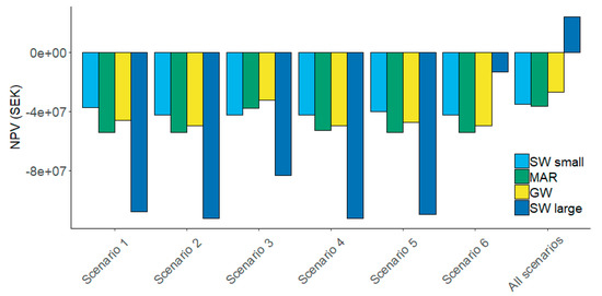
Figure 5.
Net present values for measure implementation with the annual benefit of risk reduction for each individual risk scenario and for all scenarios combined, over a 50-year time horizon and with 3.5% discount rate (mean values).
The economic benefit of risk reduction is distributed differently across households, businesses and the municipality for the analyzed measures and scenarios. In Scenario 1, the municipality gained 100% of the benefits. In Scenario 2, no measure contributed with any benefit of risk reduction. In Scenario 3, the households gained 100% of the benefits. In Scenario 4, the households gained 100% of the benefits of MAR. The other measures did not contribute to any benefits in that scenario. In Scenario 5, the municipality gained 99.7% of the benefits of the increased groundwater extraction and the small- and large-scale surface water measures, and the households gained 0.3% of the benefits. In Scenario 6, the businesses gained 99.2% of the benefits of the large-scale surface water measure and the households gained 0.8%. No other measure contributed with risk reduction in that scenario.
Results from the two forms of sensitivity analyses performed (based on scenario analysis and Monte Carlo simulations respectively) are provided in Table 5 and Figure 6. Table 5 shows that the ranking order of the measures did not vary much when applying different discount rates. However, the order of the measures varied when applying different price elasticities. Particularly the MAR measure benefited from the −0.2-price elasticity compared to the other measures.

Table 5.
Ranking order of net present values for analyzed measures when using two different price elasticities of water demand and three different discount rates. Rank 1 = highest net present value (NPV) and Rank 4 = lowest NPV (mean values). The risk reduction of all scenarios combined are used in these calculations.
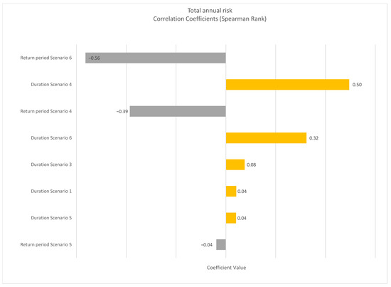
Figure 6.
Correlation coefficients (Spearman rank) of the eight most strongly correlated input variables for the total annual risk.
Figure 6 shows the degree to which input variables co-vary with the calculated total risk, expressed using Spearman rank correlation coefficients between −1 and 1. Input variables related to the return periods and duration of the risk scenarios contributed more to the outcome uncertainty than input parameters related to the economic consequences of the scenarios. This holds true also when comparing how the input variables co-vary with the estimated NPVs, i.e., input variables related to return periods and duration of risk scenarios contributed most to the NPV uncertainties.
5. Discussion
Gotland’s drinking water system is vulnerable to supply and demand fluctuations. Insufficient water availability in combination with rainfall deficiencies and large seasonal demand variations pose challenges to the local water utility. In addition, the total water demand on the island is expected to increase by more than 40% over the coming decades [38]. Taken together, the low and varied water availability coupled with other threats to the drinking water system, illustrates the importance of understanding the system risks as well as the benefits of investing in a reliable water supply [14]. In this paper, four potential risk reduction measures were analyzed for Gotland, providing guidance on how efficient the measures are to reduce different types of risks. The risk analysis was combined with cost-benefit analysis to provide information on the measures’ economic viability. For Gotland, the large-scale surface water measure (SW large) proved to be the most beneficial measure for reducing the risk in most individual risk scenarios and in all scenarios combined. However, the large-scale surface water measure was the least economically beneficial measure for the individual Scenarios 1 to 5 when comparing NPVs, but the most economically beneficial measure for Scenario 6 and when including the risk reduction of all scenarios combined. This is because the measure has high implementation costs but also a high risk reduction effect on several of the scenarios, and the combined effect of these risk reductions creates a large benefit. The varying ranking order of the measures for Gotland, when analyzing risk reductions for individual scenarios versus all scenarios combined, highlights the importance of a holistic risk assessment, integrating a range of risk scenarios. This is to avoid sub-optimization where measures are prioritized based on individual risk scenarios. By calculating the total risk, the possibility of more than one scenario occurring simultaneously is considered. However, it should be noted that the measures analyzed in this paper focused mostly on improving the raw water system, and little attention was given to improving the treatment system or the distribution system.
The presented method makes use of a non-overlapping subset of risk scenarios, which together should represent all possible scenarios for water supply disruptions. By quantifying the probability of losses caused by the scenarios, a risk curve is produced showing the relationship between frequency and its associated losses. Each point of the curve represents the actual return period of losses, and the curve can hence be used to provide information on how to address the different levels of risk. In the paper, we have chosen to express the risk in terms of expected economic consequences to society arising from disruption events. However, it is important to point out that in other situations there may be reasons to express the risk in other terms, in which case the same method can still be used. It is also important to note that there are limitations in expressing the risk in terms of expected consequences, particularly when it comes to capture events with low probabilities and high consequences [18]. However, we have judged the type of events we consider are the type that can be assessed with expected consequences.
Rational decision-making requires that the risks, along with other costs and benefits, are properly accounted for in the decision-making process [9]. However, evaluations of alternative measures and their effects will always comprise uncertainties. In this paper, the uncertainties of input variables were represented by probability distributions, and the uncertainty of the outcomes were calculated by means of Monte Carlo simulations. This approach allows us to study the uncertainty in the results and the likelihood of each outcome. It also facilitates sensitivity analysis, e.g., using Spearman rank correlation coefficients, to study how uncertainties of specific input variables contribute to the uncertainties in the results. Such information can for example be used to support decisions on which input variables to prioritize for further research and/or data collection in order to reduce uncertainties in results. However, it is practically impossible to cover all aspects of real systems [24]. Hence, the assigned probabilities are conditioned on several assumptions and simplifications. For assumptions and simplifications not to be overlooked in the risk management and decision-making processes, these variables are included in the analysis using a qualitative approach as suggested by e.g., Aven [18] (p. 630). This approach highlights basic assumptions that, for example, affect the estimated input variables. If the analysis would have been based on another understating of the system and its development, the results would of course have been different. Hence, the qualitative uncertainty analysis provides transparency and is of great importance when interpreting the result. Further, some discrete uncertainties, such as discount rates and price elasticities, are analyzed by use of scenario analysis [43]. This comprehensive handling of uncertainties demonstrates a structured and transparent way of expressing risk so that water utilities can use estimates of failure rates and welfare losses over a range of disruption scenarios to identify the measures that will lead to the lowest economic losses for society, and hence improve water supply planning and risk management.
It should be emphasized that despite the abundant information provided by the risk assessment approach, its most important contribution may be that it initiates a process in which aspects otherwise likely overlooked or ignored are openly addressed. For example, definition of risk scenarios, uncertainty estimations of input variables, economic valuation of consequences, calculations of the total integral sum of risk over different risk scenarios, and calculations of economic profitability through CBA are all rare in water supply reliability studies. However, we did not consider combinations of risk reduction measures or effects on other externalities, such as health issues or agricultural production. Hence, the provided method can be improved by enabling assessments of measure combinations and inclusion of other relevant costs and benefits.
6. Conclusions
The main conclusions of this paper are:
- The risk-based approach proposed in this paper can be used to evaluate uncertainties and provide information on frequencies and welfare losses of water supply disruptions. By evaluating a range of scenarios, decision makers become aware of the strengths and weaknesses of their water supply system. An increased knowledge of the risks allows for an understanding of how to address the threats and can be used as a starting point for identifying risk reduction measures. The approach enables decision makers to build strategic capacity for operating in difficult and uncertain futures.
- In the proposed approach, alternative measures can be evaluated and compared based on their risk reduction capacities, highlighting whether they reduce the frequencies and/or the consequences of identified risk scenarios. By combining the risk analysis with cost-benefit analysis, additional information is provided on measures for leveraging investments in managing and reducing the risks. This can be used to identify the most economically profitable risk reduction alternatives.
- The approach enables an overall assessment of risk and highlights the importance of considering the full range of possible outcomes. There are advantages to evaluating the total risk based on the full spectrum of scenarios ranging from low to high probability events. Some advantages derive from the opportunity to understand how different factors influence each component of risk and how they, in turn, affect the total risk. Other advantages relate to the risk-based decision making, as the ranking and prioritization of risk reduction measures may vary depending on whether the measures are evaluated with respect to single or multiple low and/or high probability events. The case study results clearly illustrate the potential sub-optimization that may arise if measures are evaluated only based on individual risk scenarios.
Author Contributions
Conceptualization, methodology and resources, L.R., A.L. and K.S.; software, formal analysis, investigation, project administration, visualization, writing—original draft preparation, K.S.; data curation, K.S., A.L. and T.S.; funding acquisition, L.R. and K.S.; supervision, A.L. and L.R.; validation and writing—review and editing, K.S., A.L, T.S. and L.R. All authors have read and agreed to the published version of the manuscript.
Funding
This research was funded by the European Union’s Horizon 2020 research and innovation program under the Marie Skłodowska-Curie grant agreement No 754412; Region Västra Götaland; and the Swedish Research Council Formas contract no 942-2015-130.
Acknowledgments
This research was performed within the DRICKS center for drinking water research coordinated by the Chalmers University of Technology. The authors would like to thank Mikael Tiouls and Lars Westerlund, as well as all other workshop participants, at Region Gotland for contributing with Gotland-specific expertise on scenarios and societal effects.
Conflicts of Interest
The authors declare no conflicts of interest. The funders had no role in the design of the study; in the collection, analyses, or interpretation of data; in the writing of the manuscript, or in the decision to publish the results.
References
- Schlosser, C.A.; Strzepek, K.; Gao, X.; Fant, C.; Blanc, É.; Paltsev, S.; Jacoby, H.; Reilly, J.; Gueneau, A. The future of global water stress: An integrated assessment. Earth’s Future 2014, 2, 341–361. [Google Scholar] [CrossRef]
- Veldkamp, T.I.E.; Wada, Y.; Aerts, J.C.J.H.; Ward, P.J. Towards a global water scarcity risk assessment framework: Incorporation of probability distributions and hydro-climatic variability. Environ. Res. Lett. 2016, 11, 024006. [Google Scholar] [CrossRef]
- Döll, P.; Jiménez-Cisneros, B.; Oki, T.; Arnell, N.W.; Benito, G.; Cogley, J.G.; Jiang, T.; Kundzewicz, Z.W.; Mwakalila, S.; Nishijima, A. Integrating risks of climate change into water management. Hydrol. Sci. J. 2014, 60, 4–13. [Google Scholar] [CrossRef]
- Lindhe, A.; Rosen, L.; Norberg, T.; Bergstedt, O. Fault tree analysis for integrated and probabilistic risk analysis of drinking water systems. Water Res. 2009, 43, 1641–1653. [Google Scholar] [CrossRef]
- Aven, T.; Ben-Haim, Y.; Boje Andersen, H.; Cox, T.; López Droguett, E.; Greenberg, M.; Guikema, S.; Kroeger, W.; Renn, O.; Thompson, K.M.; et al. Society for risk analysis glossary. Available online: https://sra.org/sites/default/files/pdf/SRA_glossary_20150622.pdf?pdf=Glossary (accessed on 9 April 2020).
- IPCC. Climate Change 2014: Impacts, Adaptation, and Vulnerability. Summaries, Frequently Asked Questions, and Cross-Chapter Boxes. A Contribution of Working Group ii to the Fifth Assessment Report of the Intergovernmental Panel on Climate Change; World Meteorological Organization: Geneva, Switzerland, 2014. [Google Scholar]
- Government Office for Science. Blackett Review of High Impact Low Probability Risks; The National Archives: London, UK, 2011. [Google Scholar]
- Bjørnsen, K.; Aven, T. Risk aggregation: What does it really mean? Reliab. Eng. Syst. Saf. 2019, 191, 106524. [Google Scholar] [CrossRef]
- Kaplan, S.; Garrick, B.J. On the qualitative definition of risk. Risk Anal. 1981, 1, 11–27. [Google Scholar] [CrossRef]
- Lizarraga, S.A. The Economic Consequences of Water Utility Disruptions; University of Missouri: Columbia, MO, USA, 2013. [Google Scholar]
- Rose, A.; Wei, D.; Wein, A. Economic impacts of the shakeout scenario. Earthq. Spectra 2011, 27, 539–557. [Google Scholar] [CrossRef]
- Kajitani, Y.; Tatano, H. Estimation of lifeline resilience factors based on surveys of Japanese industries. Earthq. Spectra 2009, 25, 755–776. [Google Scholar] [CrossRef]
- Brozović, N.; Sunding, D.L.; Zilberman, D. Estimating business and residential water supply interruption losses from catastrophic events. Water Resour. Res. 2007, 43, 14. [Google Scholar] [CrossRef]
- Buck, S.; Nemati, M. Valuing Water Supply Reliability with Sensitivity Analysis. In Proceedings of the Southern Agricultural Economics Association’s 2017 Annual Meeting, Mobile, AL, US, 4–7 February 2017. [Google Scholar]
- Uzielli, M.; Nadim, F.; Lacasse, S.; Kaynia, A.M. A conceptual framework for quantitative estimation of physical vulnerability to landslides. Eng. Geol. 2008, 102, 251–256. [Google Scholar] [CrossRef]
- Hall, J.; Borgomeo, E. Risk-based principles for defining and managing water security. Philos. Trans. R. Soc. A 2013, 371, 20120407. [Google Scholar] [CrossRef] [PubMed]
- ISO. Iso 31000:2018 Risk Management—Guidelines; International Organization for Standardization: Geneva, Switzerland, 2018. [Google Scholar]
- Aven, T. On how to define, understand and describe risk. Reliab. Eng. Syst. Saf. 2010, 95, 623–631. [Google Scholar] [CrossRef]
- Pate-Cornell, E. On “black swans” and “perfect storms”: Risk analysis and management when statistics are not enough. Risk Anal. 2012, 32, 1823–1833. [Google Scholar] [CrossRef] [PubMed]
- Jenkinson, D. The Elicitation of Probabilities—A Review of the Statistical Literature; Department of Probability and Statistics, Sheffield, University of Sheffield: Sheffield, UK, 2005. [Google Scholar]
- Werner, C.; Bedford, T.; Cooke, R.M.; Hanea, A.M.; Morales-Nápoles, O. Expert judgement for dependence in probabilistic modelling: A systematic literature review and future research directions. Eur. J. Oper. Res. 2017, 258, 801–819. [Google Scholar] [CrossRef]
- O’Hagan, A.; Buck, C.E.; Daneshkhah, A.; Eiser, J.R.; Garthwaite, P.H.; Jenkinson, D.J.; Oakley, J.E.; Rakow, T. Uncertain Judgements: Eliciting Experts’ Probabilities; John Wiley & Sons: West Sussex, UK, 2006. [Google Scholar]
- Johansson, P.-O.; Kriström, B. Cost-Benefit Analysis for Project Appraisal; Cambridge University Press: Cambridge, UK, 2016. [Google Scholar]
- Kaplan, S.; Haimes, Y.Y.; Garrick, B.J. Fitting hierarchical holographic modeling into the theory of scenario structuring and a resulting refinement to the quantitative definition of risk. Risk Anal. 2001, 21, 807–819. [Google Scholar] [CrossRef]
- Oakley, J.E.; O’Hagan, A. Shelf: The Sheffield Elicitation Framework (Version 3.0). Available online: http://tonyohagan.co.uk/shelf (accessed on 11 April 2019).
- Morris, D.E.; Oakley, J.E.; Crowe, J.A. A web-based tool for eliciting probability distributions from experts. Environ. Model. Softw. 2014, 52, 1–4. [Google Scholar] [CrossRef]
- VASS. Swedish Water and Wastewater Assoication’s Statistics System. Available online: http://www.vass-statistik.se/ (accessed on 19 September 2018).
- Sebri, M. A meta-analysis of residential water demand studies. Environ. Dev. Sustain. 2013, 16, 499–520. [Google Scholar] [CrossRef]
- Höglund, L. Household demand for water in sweden with implications of a potential tax on water use. Water Resour. Res. 1999, 35, 3853–3863. [Google Scholar] [CrossRef]
- FEMA. Fema Benefit-Cost Analysis Re-Engineering (BCAR). Development of Standard Economic Values; Federal Emergency Management Agency (FEMA): Washington, DC, USA, 2011. [Google Scholar]
- Gotland County Regional Economy (Regionfakta). Available online: http://www.regionfakta.com/gotlands-lan/regional-ekonomi/brp-per-bransch-och-sektor/ (accessed on 8 January 2020).
- ATC. Atc-25. Seismic Vulnerability and Impact of Disruption of Lifelines in the Conterminous United States; FEMA Federal Emergency Management Agency: Washington, DC, USA, 1991. [Google Scholar]
- Lindhe, A.; Rosen, L.; Norberg, T.; Bergstedt, O.; Pettersson, T.J. Cost-effectiveness analysis of risk-reduction measures to reach water safety targets. Water Res. 2011, 45, 241–253. [Google Scholar] [CrossRef]
- Stern, N. Stern Review: The Economics of Climate Change; Grantham Research Institute on Climate Change and the Environment, Her Majesty’s Treasury of the UK Government: London, UK, 2006. [Google Scholar]
- Swedish Transport Administration. Analysis Method and Socio-Economic Cost and Benefit Values for the Transport Sector: Asek 6.1.; Swedish Transportation Administration: Borlänge, Sweden, 2018. [Google Scholar]
- Van Westen, C.J.; Quan Luna, B.; Vargas Franco, R.D.; Malet, J.P.; Jaboyedoff, M.; Horton, P.; Kappes, M. Development of Training Materials on the Use of geo—Information for Multi-hazard Risk Assessment in a Mountainous Environment. In Proceedings of the International Conference on Mountain Risks: Bringing Science to Society, Firenze, Italy, 24–26 November 2010; pp. 469–475. [Google Scholar]
- Dahlqvist, P.; Sjöstrand, K.; Lindhe, A.; Rosén, L.; Nisell, J.; Hellstrand, E.; Holgersson, B. Potential benefits of managed aquifer recharge mar on the island of Gotland, Sweden. Water 2019, 11, 2164. [Google Scholar] [CrossRef]
- Eklund, F. Regional Water Supply Plan of Gotland; County Administrative Board of Gotland: Visby, Sweden, 2018. [Google Scholar]
- Westerlund, L.; Tiouls, M. Personal Communication; Region Gotland: Visby, Sweden, 2020. [Google Scholar]
- Region Gotland. Gotland in Numbers (Gotland i Siffror). Available online: https://www.gotland.se/64224 (accessed on 12 September 2018).
- Sjöstrand, K.; Lindhe, A.; Söderqvist, T.; Dahlqvist, P.; Rosén, L. Marginal abatement cost curves for water scarcity mitigation under uncertainty. Water Resour. Manag. 2019, 33, 4335–4349. [Google Scholar] [CrossRef]
- Region Gotland. Vision and Strategy for Gotland’s Water Supply 2030; Region Gotland: Visby, Sweden, 2017. [Google Scholar]
- Parnell, G.S.; Bresnick, T.; Tani, S.N.; Johnson, E.R. Handbook of Decision Analysis; John Wiley & Sons, Incorporated: Hoboken, NJ, USA, 2013. [Google Scholar]
© 2020 by the authors. Licensee MDPI, Basel, Switzerland. This article is an open access article distributed under the terms and conditions of the Creative Commons Attribution (CC BY) license (http://creativecommons.org/licenses/by/4.0/).

