Estimation of Surface Water Runoff for a Semi-Arid Area Using RS and GIS-Based SCS-CN Method

Abstract

The proper planning of storage structures, waterways, irrigation schemes, water harvesting, erosion control structures, and groundwater development strategies requires accurate estimation of surface runoff. However, hydrologists in Saudi Arabia face serious challenges, specifically due to the rare availability of surface runoff data. In this study, the soil conservation service-curve number (SCS-CN) method integrated with geographic information system (GIS) and remote sensing (RS) was utilized to estimate the surface runoff in Wadi-Uranah basin, in the western region of Saudi Arabia. Different thematic maps such as slope, hydrologic soil group (HSG), land use/land cover (LULC), and daily rainfall have been created in GIS environment and processed to generate the curve number (CN) and surface runoff maps. Based on the soil classification results, the study area was categorized into two HSGs (B and C). The dominant HSG was group C, representing about 98.8% of the total area. The LULC analysis showed four main land use types in the study region: urban, rocks, barren soil, and agricultural areas. Furthermore, the finding results showed that CN values for the normal conditions (CN_II) ranged between 74 and 93 in agricultural and both urban and rock areas, respectively. The CN_II values were further corrected using slope data to derive slope-adjusted CN_II. Moreover, the rainfall-runoff results showed an increase in the daily runoff of the study region with a minimum of 15 mm to a maximum of 74 mm. Another interesting result was rainfall-runoff linear regression analysis that showed a good correlation of 0.98. Additionally, the peak runoff hydrograph flows for 10-, 50-, and 100-year return periods obtained from the SCS-based dimensionless unit hydrograph were 828, 1353, and 1603 m³/s, respectively. Therefore, this study highlights that the SCS-CN method integrated with RS and GIS deserves further attention for estimating runoff of ungauged basins for better basins management and conservation purposes.

1. Introduction

Watershed runoff plays an important role in designing hydraulic structures, controlling soil erosion, and assessing the water yield potential of the watershed [1,2]. To overcome water scarcity challenges that most arid and semi-arid regions face such as Saudi Arabia, decision-makers in that region must come up with strategies to explore new water resources or optimize the usage of the available resources. However, the provision of accurate information about runoff is barely available due to the high installation and maintenance costs of the hydrologic gauging stations. Accordingly, reliable information on watershed runoff must be continuously developed to facilitate the creation and management of watershed programs [3].

In the absence of runoff measurements, estimated direct runoff has shown accurate results via soil conservation service-curve number (SCS-CN), a model developed by hydrologists at the Department of Agriculture of the United States [4,5,6]. The SCS-CN model combines the parameters of the watershed with the climatic factors in a single entity called the curve number (CN). A high CN indicates low infiltration and high runoff, while a low CN implies high infiltration and low runoff. The SCS-N method provides adequate results without using complex data [7,8,9,10]. For instance, Liu and Li [11] computed the runoff over a watershed in the Loess Plateau of China with the SCS-CN method, and stated that the SCS-CN is an effective and successful method for estimating runoff. Moreover, Topno et al. [12] employed the SCS-CN model for simulating the annual depth of runoff over an ungauged catchment (Vindhyachal region). They revealed that the SCS-CN method can be used efficiently to estimate the depth of runoff when there is no adequate hydrological information.

The SCS-CN method is mainly influenced by significant runoff-associated watershed features such as land use/land cover (LULC), hydrologic soil group (HSG), slope, and climate conditions [13,14,15]. The term LULC defines how a specified area is exploited. The usage of LULC can take many forms, including water bodies, built-up land, agricultural land, barren land, and roads [16]. The expression HSG was introduced by the National Resources Conservation Service (NRSC). NRSC classified soil types having the same physical features and runoff characteristics into specified HSGs groups [17]. These HSGs namely A, B, C, D, A/D, B/D, and C/D have been rated in descending order to the infiltration rate. In other words, Group A refers to soils with high rates of infiltration (low potential runoff) while group D refers to soils that have low rates of infiltration (high potential runoff). Soil types which have moderate and low infiltration rates are classified as group B and C, respectively [17].

According to the effect of the slope on the SCS-CN model, it has been demonstrated that the slope can affect the estimated surface runoff in three ways, including initial abstraction reduction [18], infiltration reduction [19], and decrease of the recession time of overland flow [20]. In the Loess Plateau (China), Fang et al. [21] found that greater gradients of the slope can lead to larger flow velocities, which gives less time for rainfall to be infiltrated into the soil on one hand, and on the other hand, increase the runoff generation capacity. Furthermore, Chaudhary et al. [22] and Jha et al. [23] have experimentally investigated the impact of watershed slope on the generation of runoff and CN for a given soil (HSG with class C) and sugarcane. They found that the higher the slopes, the greater the runoff and vice-versa.

The CN can be calculated from the readily available tables and curves, but this traditional method is very tedious besides, it consumes a large portion of hydrologic modeling time. In contrast, the use of the geographic information system (GIS) and remote sensing (RS) together with hydrologic models gives considerable reduction in both the cost and time with high reliability and accuracy over the traditional methods [24]. Globally, many studies have been conducted using GIS and RS techniques to simulate the surface runoff [25]. Nayak and Jaiswal [26] found that the measured and simulated depths of the runoff by the GIS based SCS-CN method were well correlated. Geena and Ballukraya [27] conducted a study in red hills watershed thereby developed CNs suited for Indian conditions using the SCS-CN method and GIS. In their study, they found that the GIS and RS tools can be accurately used to estimate the spatial hydrological parameters and temporal variables. Another study was carried out by Gitika and Ranjan [28] in the Buriganga watershed (India) to estimate the surface runoff using the GIS and RS technologies. The study results concluded that both the GIS and RS technologies are powerful tools for estimating runoff generation in the geo-hydrologic environment. The objective of this study was to apply the RS and GIS-based SCS-CN model for simulating the surface runoff to support the decision-making process for the future development of water resources and hydraulic structures in the area.

2. Materials and Methods

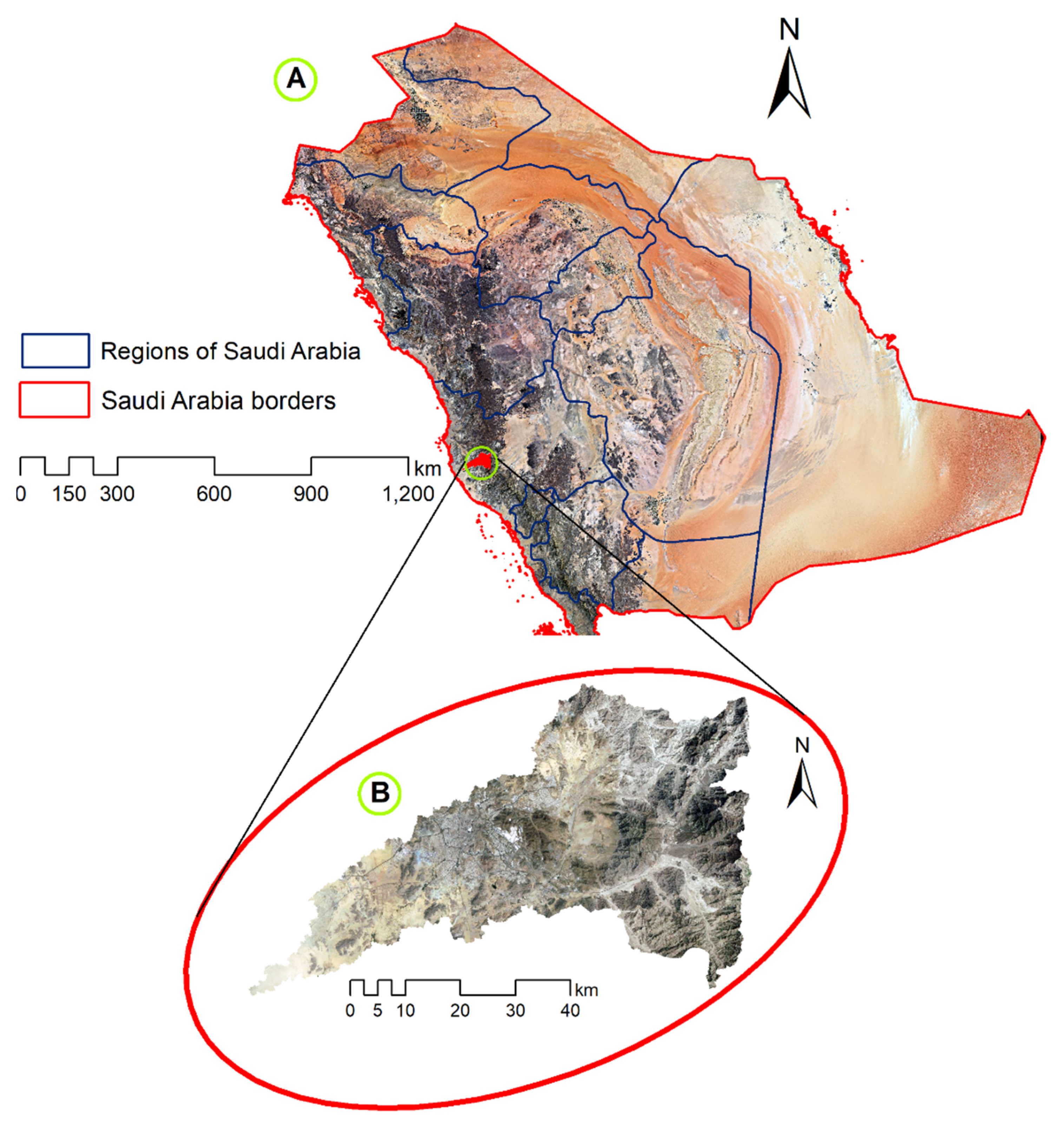
2.1. Description of the Study Area

This study was conducted at the Wadi-Uranah basin located in the western region of Saudi Arabia. The basin considered in this study is geo-graphically located within the latitude of 21°01′30′ N to 21°30′30′ N and longitude of 39°12′00′ to 40°18′00′ E. The basin covers a total area of about 2121.5 km², with an elevation ranges from 53 to 2510 m above mean sea level (Figure 1). Wadi-Uranah’s upstream consists of four sub-basins, the Wadi-Numan, Wadi-Al-Sharaea, Wadi-Ibrahim and Wadi-Mehassar, all of which stream into Makkah’s central area. Wadi-Ibrahim and Wadi-Mehassar are both located within Makkah’s urban areas, while Wadi-Numan (749 km²) and Wadi-Al-Sharaea (657 km²) have fewer built-up areas compared to their total areas. The weather is characterized by monsoon climate with dry and wet seasons [29]. The average annual rainfall in the study area is about 101 mm [30]. Furthermore, there are remarkable climatic conditions, particularly the sandy storms and torrential rains.

2.2. Data and Software

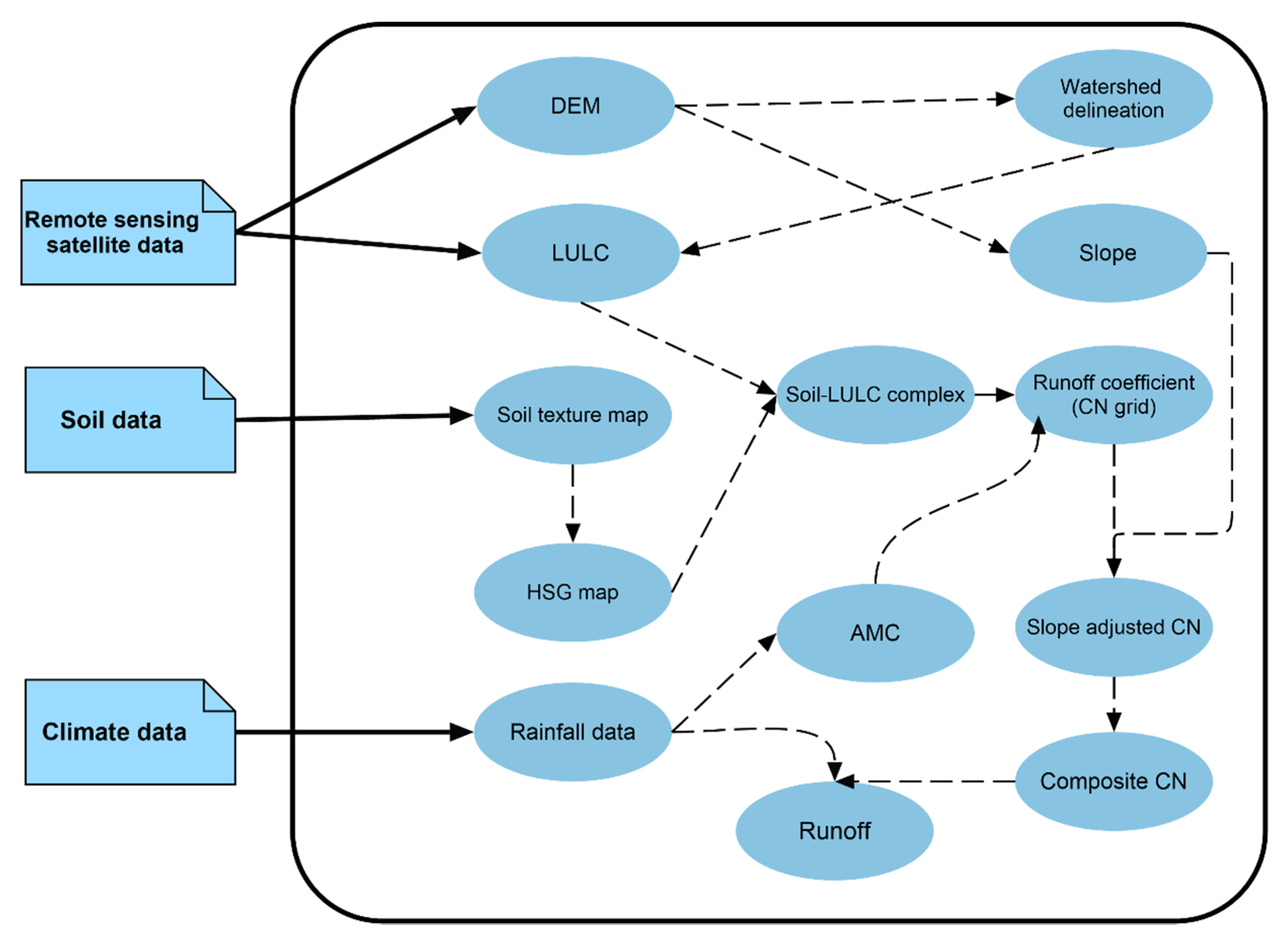
For a period of 35 years, the rainfall data of the study region was obtained through the Climate Prediction System Reanalysis (CFSR). Soil data was derived from general soil map of Saudi Arabia, Ministry of Environment, Water and Agriculture (MEWA). A Landsat satellite imagery downloaded from the United States Geological Survey (USGS) was used to develop the land use/land cover (LULC) map of the study region. Specifications of the satellite data acquired for LULC analysis are given in

Table 1. Details of acquired satellite image.

Satellite	Sensor	Path/Row	Acquisition Date	Spatial Resolution
Landsat 8	ETM	169/45	3 March 2020	30 m

. A digital elevation model (DEM) with a resolution of 30 m was downloaded from the USGS to derive the elevation, slope, stream network and extents of the basin for the study area (Figure 2). ArcGIS 10.5 and ERDAS Imagine 2015 software were used to build, manage, and generate various layers and maps.

2.3. Methodology

Figure 3 shows the overall methodology employed by the geographic information system (GIS) and soil conservation service-curve number (SCS-CN) method in estimating the surface runoff within the studied region. The GIS-based data base was used for building of LULC and hydrological soil group (HSG) shapefiles. HSG and LULC shapefiles were intersected in GIS environment to produce new and smaller polygons associated with names of HSG and LULC. Based on the intersected LULC-HSG layer and its associated attribute table, the curve number (CN) database was constructed. The CN grid map was then generated from the DEM, LULC-HSG and CN database which all are required as inputs in GIS. A further correction was made to the created CN map using slope data to derive slope-corrected CN map. Finally, the raster calculator function in the GIS software was used to calculate the surface runoff depth from the slope-corrected CN map and rainfall data.

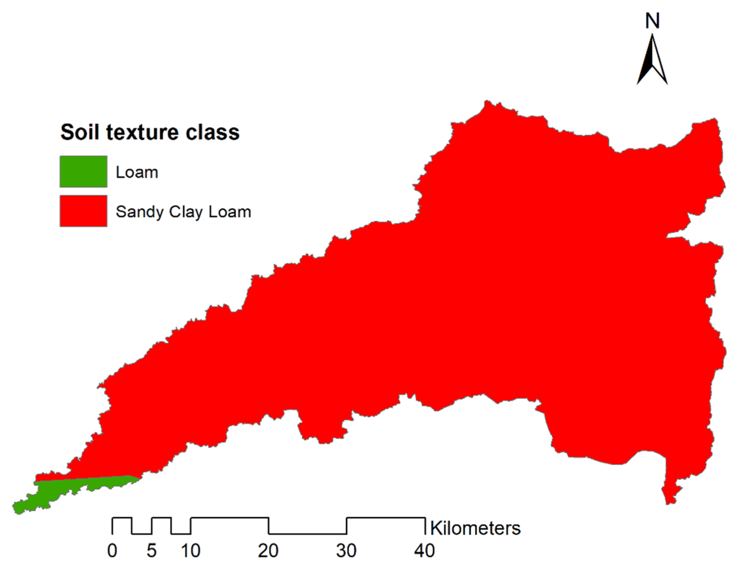
2.4. Soil Texture Map

The texture of the soil is very important for determining the HSG. It is a basic parameter to study the soil-water relation and the hydraulic characteristics of the soils [31,32]. Soil textures are categorized according to different fractions of each soil (sand, silt, and clay). Typically, classifications are given for the main constituent particle size or a combination of the most abundant particle sizes. A soil textural class map of Wadi-Uranah basin was developed by the GIS-based soil data acquired from the MEWA (Figure 4). Two different kinds of soil texture, namely sandy clay loam and loam were found in the study region. A 98.81% of the region is sandy clay loam soil, which is characterized by low infiltration rates while remaining area (1.19%) is loam soil, which has a moderate infiltration rate (Figure 4). For both the sandy clay loam and loam soils, the saturated hydraulic conductivity of the least transmissivity layer ranges from 1.5 to 5.1 cm/h.

2.5. Hydrologic Soil Group Map

Based on the map of soil textures, soil of the Wadi-Uranah basin was classified into two HSGs: B and C (Figure 5). As shown in Figure 5, the HSG with class C (HSG-C) occupies approximately 2096.4 km², which is 98.81% of the basin’s total area whilst 1.19% of the total coverage area is HSG-B. The dominance of HSG-C indicates that the soils in the basin have a moderately fine-to-fine structure, with a slow rate of water transmission and slow rate of infiltration when thoroughly wetted. Regarding HSG-B, it has a moderate infiltration rate when thoroughly wetted and consists mainly of moderately deep to deep, moderately well to well-drained soils, with moderately fine to moderately coarse textures. Considering the relative proportion of the HSG, it can be concluded that most of the soils in the Wadi-Uranah basin contribute a large amount of surface runoff, and a small to medium proportion of the precipitation is only infiltrated into the soil.

2.6. Land Use/Land Cover

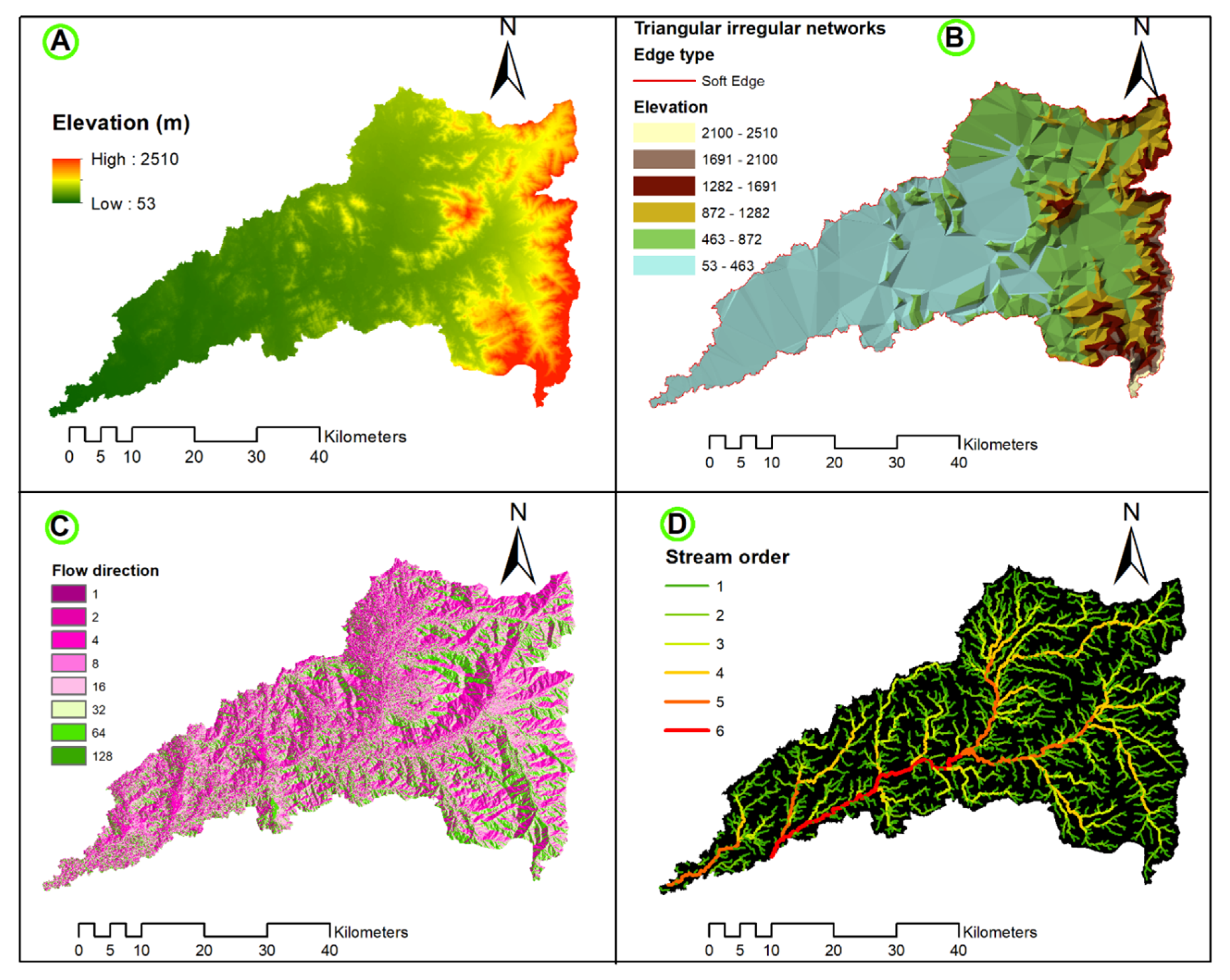
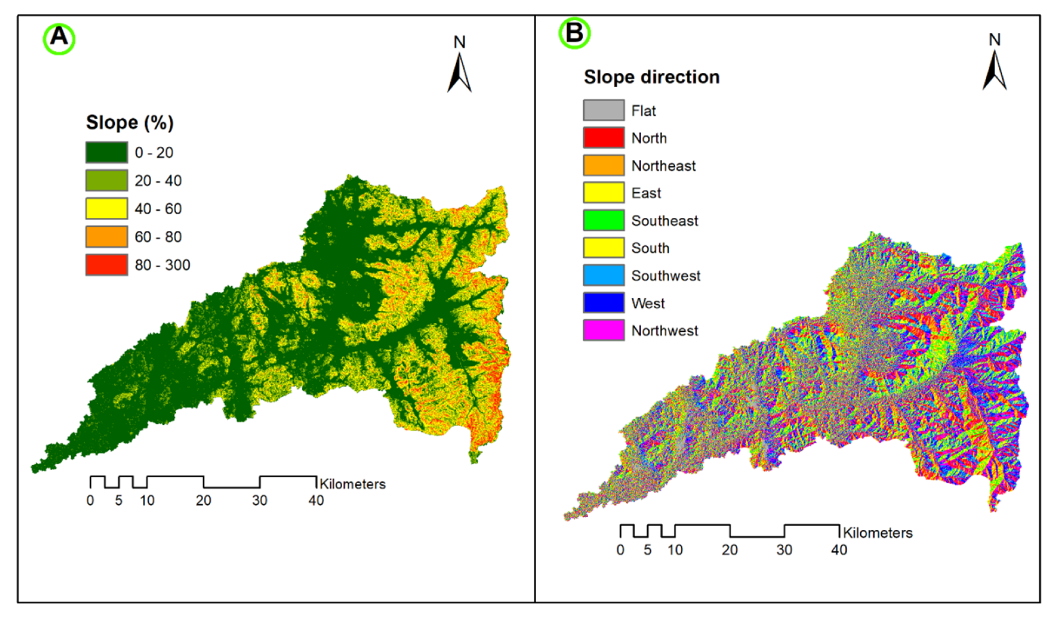
LULC is one of the main thematic inputs of any hydrological analysis, since it provides the current status of land use and patterns. The LULC map of the study region was developed with the help of Landsat-8 ETM satellite imagery (30 m resolution) obtained from the USGS. The pan-sharpening algorithm in ArcGIS was used to produce pan-sharpened high-resolution multispectral images (15 m) by combining the high resolution panchromatic (15 m) and low resolution multispectral (30 m) images. The maximum likelihood classifier function in ERDAS Imagine 15 was employed to classify the area of study into different classes of LULC. For identifying what the cluster represents, spectral signatures collected from training samples were used (polygons representing distinct sampling areas of the various types of LULC to be classified).

2.7. Slope Map

A slope is an inclined ground surface forming an angle with the horizontal plane. A DEM with 30 m resolution was used to produce the slope and aspect analysis of the Wadi-Uranah basin. In order to ensure the continuity of water flow to the outlet of the basin, the DEM was analyzed using ArcGIS software as a pre-processing phase to eliminate sinks and flat areas. The slope map of the Wadi-Uranah basin is shown in Figure 6A. As shown in Figure 6A, values of basin slope vary from 0 to 300%, with an average value of 23%. Study area slopes were categorized into five main classes: very low (<20%), low (20–40%), medium (40–60%), high (60–80%), and very high (>80%). Each class occupies a percentage of 56%, 19%, 16%, 7%, and 2% of the studied area, respectively. The aspect map that was generated by ArcGIS software for the study area is shown in Figure 6B. As shown in Figure 6B, the area of interest is sloping from the southeast to the west.

2.8. The Soil Conservation Service Runoff Estimation Method

The SCS method of runoff is based on the CN, which quantifies the impact of soil and land cover on the processes of rainfall- runoff. The SCS model of runoff [4] is given in Equation (1):

$$\mathrm{Q}=\{\begin{array}{ll}\frac{{\left(\mathrm{P}-\mathsf{\lambda }\mathrm{S}\right)}^2}{\mathrm{P}+\left(1-\mathsf{\lambda }\right)\mathrm{S}}& \mathrm{P}>\mathsf{\lambda }\mathrm{S}\\ 0& \mathrm{P}\le \mathsf{\lambda }\mathrm{S}\end{array}$$

(1)

where Q; P; λ; and S are direct runoff; total rainfall; initial abstraction coefficient; and potential maximum retention, respectively.

In Equation (1), λS is equal to the initial abstraction that accounts for infiltration, canopy interception, and storage of surface depression during the early part of the storm [33]. Mishra and Singh [34] noted that λ may vary between 0 and ∞. However, for general use, λ = 0.2 is recommended [35]. The S value for the CN derived from the characteristics of the basin can be calculated as:

$$\mathrm{S}=\frac{25400}{\mathrm{CN}}-254$$

(2)

where CN is a dimensionless parameter with a value between 0 (no runoff, S = ∞) and 100 (all rainfall becomes runoff, S = 0). It is determined by HSG, LULC, and antecedent soil moisture condition (AMC). AMC is pre-storm indicator of basin wetness and soil storage availability. In CN method, three levels of AMC are used: AMC-I for dry, AMC-II for normal, and AMC-III for wet conditions. The seasonal rainfall limits for these three AMCs are given in

Table 2. Classification of the antecedent soil moisture condition and the related curve number (CN).

AMC	Curve Number	5-Days Antecedent Rainfall (mm)
		Growing Season	Dormant Season
I	CNI	<35.6	<12.7
II	CNII	35.6–53.3	12.7–27.9
III	CNIII	>53.3	>27.9

. The CN_II for the case of AMC-II was considered in this study [7]. However, The CN_II can be converted into (CN_I) and (CN_III) associated with (AMC-I) and (AMC-III), respectively, through the Equations (3) and (4) shown below [36]:

$${\mathrm{CN}}_{\mathrm{I}}=\frac{4.2 \times {\mathrm{CN}}_{\mathrm{II}}}{10 -\left(0.058 \times { \mathrm{CN}}_{\mathrm{II}}\right)}$$

(3)

$${\mathrm{CN}}_{\mathrm{III}}=\frac{23\times \mathrm{C}{\mathrm{N}}_{\mathrm{II}}}{10+\left(0.13\times \mathrm{C}{\mathrm{N}}_{\mathrm{II}}\right)}$$

(4)

where CN_I is a curve number applied for antecedent dry condition, CN_II is a curve number applied for normal condition, and CN_III is a curve number applied for antecedent wet condition.

For a basin with sub-areas having different land uses and soil types, a composite curve number (CN_c) is determined by weighting of CN values for different sub-areas. Based on McCuen [37], the CN_c can be computed using the Equation (5) shown below [36]:

$${\mathrm{CN}}_{\mathrm{c}}={\displaystyle \sum _{\mathrm{i}=1}^{\mathrm{n}}\frac{{\mathrm{CN}}_{\mathrm{i}}\times { \mathrm{A}}_{\mathrm{i}}}{\mathrm{A}}}$$

(5)

where CN_c is the composite CN; CN_i is the CN value of the sub-region; A_i is the area of the sub-region; and A is the total basin area.

2.9. Slope-Adjusted CN_II

From the hydrology study point of view, it is essential to incorporate the slope values in CN and adjust the CN values accordingly. For the calculation of slope-adjusted CN values, the Huang et al. [13] approach was used to make the improvement and to incorporate the slope factor into the analysis (Equation (6)).

$${\mathrm{CN}}_{\mathrm{II}\mathsf{\alpha }}=\left(\frac{{\mathrm{CN}}_{\mathrm{III}}-{\mathrm{CN}}_{\mathrm{II}}}{3}\right)\left(1 -{ 2\mathrm{e}}^{-13.86\mathsf{\alpha }}\right){+\mathrm{CN}}_{\mathrm{II}}$$

(6)

where CN_IIα is slope-adjusted CN for normal conditions; CN_II and CN_III are tabulated curve number dependent on basin characteristics for normal and wet conditions, respectively; and α is the average slope of the basin (m/m).

2.10. The Soil Conservation Service Unit Hydrograph

A basin unit hydrograph is defined as a direct runoff hydrograph that results from a unit volume of excess rainfall of constant intensity, which is distributed uniformly over the drainage area [38]. The SCS method for generating a synthetic unit hydrograph is relied on a dimensionless unit hydrograph [39]. This dimensionless unit hydrograph was designed from a large number of natural unit hydrographs that developed from gauged basins with a wide range of sizes and geographical locations [40]. Both the peak time and peak discharge of the unit hydrograph are computed using the Equations (7) to (9), respectively [41]:

$${\mathrm{T}}_{\mathrm{p}}=\frac{{\mathrm{T}}_{\mathrm{r}}}{2}+{\mathrm{T}}_{\mathrm{LAG}}$$

(7)

$${\mathrm{T}}_{\mathrm{LAG}}=\frac{0.00136{\left(\mathrm{L}\right)}^{0.8}{\left(\frac{\mathrm{S}}{25.4}+1\right)}^{0.7}}{\sqrt{\mathrm{B}\mathrm{S}}}$$

(8)

$${\mathrm{q}}_{\mathrm{p}}=\frac{0.208\times \mathrm{A}\times \mathrm{Q}}{{\mathrm{T}}_{\mathrm{p}}}$$

(9)

where T_p is the time from the start of the rainfall excess up to the peak discharge (h); T_r is the duration of rainfall excess (h); T_LAG is the lag time between the center of rainfall excess and the peak discharge (h); L is the maximum distance of flow (m); BS is the average basin slope (%); S is the potential maximum retention calculated from the CN (mm); q_p is the peak discharge (m³/s); Q is direct runoff (mm); and A is the basin area (km²).

2.11. Rainfall Data

Time series rainfall records (1979–2014) acquired from the CFSR were analyzed to investigate the behavior of the maximum daily rainfall data with different N-year return periods (10, 50, and 100 years). The temporal analysis of the rainfall data was based on the probability distribution of Log Pearson Type III, which is highly recommended for the hydrological analysis [42]. For interpolating the rainfall map of the study region, the inverse square distance weighting method (Equations (10) to (12)) was used. In this method, the interpolated value is determined by the observations of weighted values, which are computed in such a way that points close to each other get large weights and points further away get small weights [43]. The weights are inversely proportional to the distance between the interpolation point and the observation point considered [43].

$$\mathrm{P}\left({\mathrm{x}}_0,{\mathrm{y}}_0\right)={\displaystyle \sum _{\mathrm{i}=1}^{\mathrm{m}}{\mathrm{w}}_{\mathrm{i}}\times {\mathrm{P}}_{\mathrm{i}}}$$

(10)

$${\mathrm{w}}_{\mathrm{i}}=\frac{1/{\mathrm{x}}_{\mathrm{i}}^2}{{\displaystyle \sum _{\mathrm{i}=1}^{\mathrm{m}}1/{\mathrm{x}}_i^2}}$$

(11)

$${\mathrm{x}}_i^2={\left({\mathrm{x}}_{\mathrm{i}}-{\mathrm{x}}_0\right)}^2+{\left({\mathrm{y}}_i-{\mathrm{y}}_0\right)}^2$$

(12)

where P (x₀, y₀) is the estimated rainfall at coordinates (x₀, y₀); P_i is the rainfall at the given station i; w_i is the station weight; and x_i = (x_i, y_i) is the coordinates of the station.

3. Results and Discussion

3.1. Rainfall Map

Rainfall data need to be spatially distributed for hydrological simulation input. For this reason, the spatial distribution map of the maximum daily precipitation over the Wadi-Uranah basin was constructed (Figure 7). It is obvious from Figure 7 that the maximum daily rainfall varies from 47 to 65 mm. The reason for this variation is that the area of concern is located in the Arabian Shield, which, on the one hand, is an elevated area and, on the other hand, forms a barrier parallel to the Red Sea. In turn, this creates diversity in the geographic distribution of the rainfall in the area being studied.

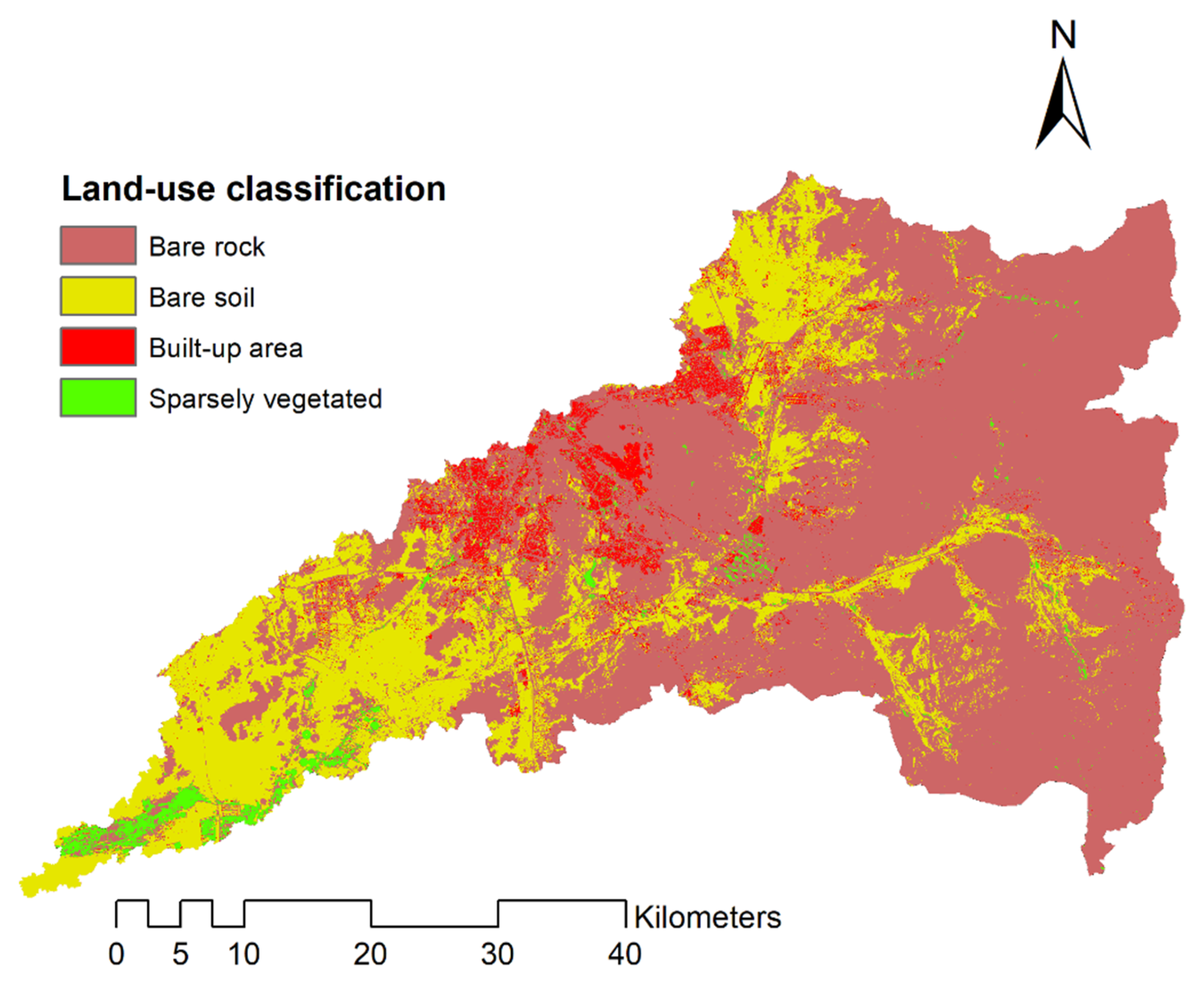
3.2. Land Use/Land Cover Map

Using the techniques described in Section 2.6, four major LULC classes were found, i.e., bare rocks, bare soils, built-up areas and agricultural land (Figure 8). The bare rocks which cover 69% of the total area were the most predominant LULC. Bare soils and built-up areas were found to cover approximately 25% and 4% of the total area, respectively. As for the vegetation, it is clear that the basin has a low vegetation cover (2%). Overall, a strong relationship between rainfall and runoff could be observed as a result of low vegetation coverage. Similar results were obtained by Zhao et al. [44] which indicated that there is a strong relationship between runoff volume and vegetation cover, where a high runoff volume was observed as a result of vegetation removal and urbanization.

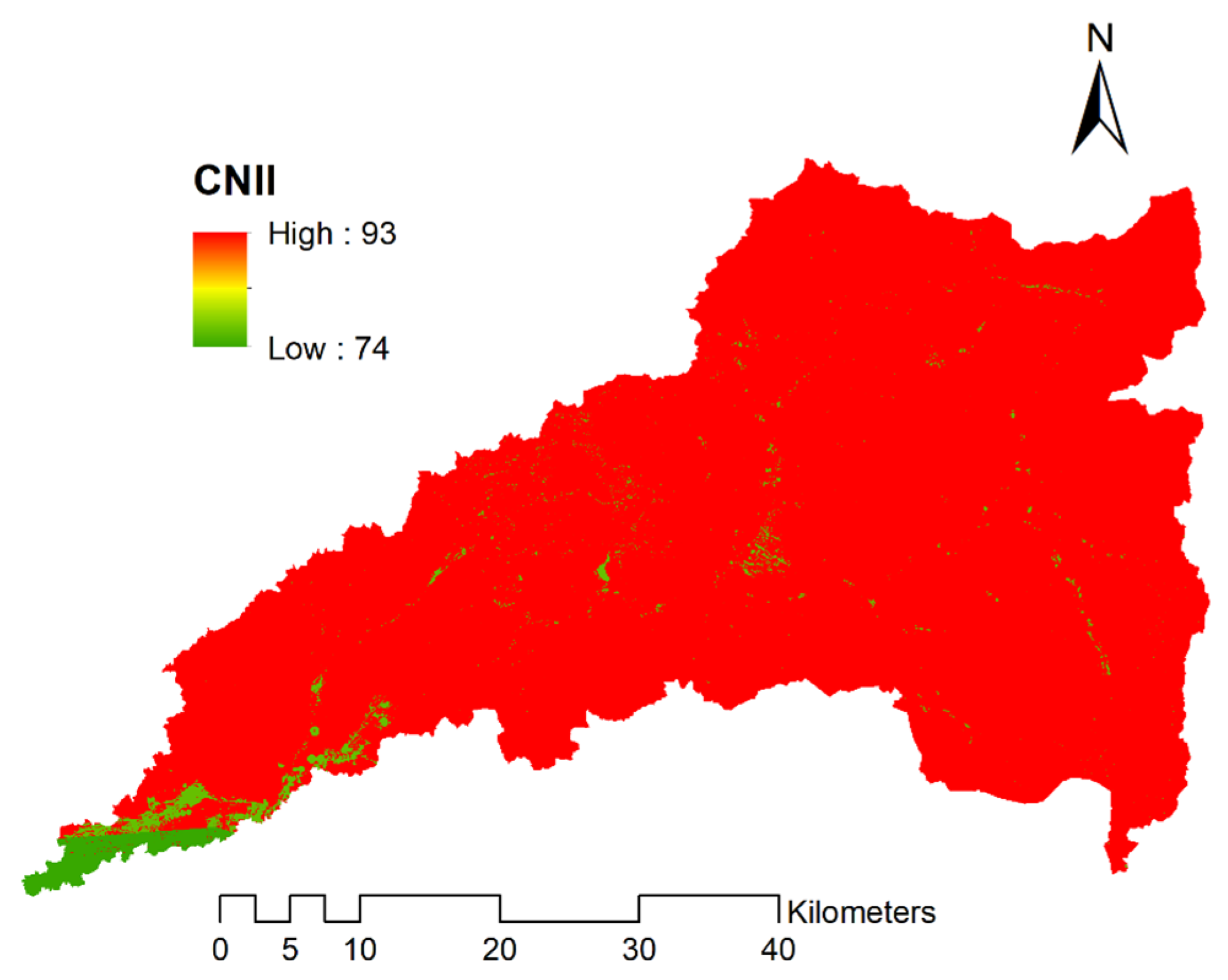
3.3. The Soil Conservation Service-Curve Number Map

The SCS-CN values for each cell were derived by the ArcGIS software on the basis of the AMC-II, HSG map, and LULC map (Figure 9). As shown in Figure 9, the values of CN_II range from 74 in agricultural areas to 93 in urban and bare rock areas. Additionally, CN_I and CN_III values associated with AMC-I and AMC-III, respectively, were determined using Equations (3) and (4) (Figure 10A,B). Figure 10A,B show that the lowest CNs values were found to be 54 and 87, whereas the highest CNs values were 85 and 97 for CN_I and CN_III, respectively. These CN_I, CN_II, and CN_III values emphasize that the Wadi-Uranah basin has many places with high impermeable zones, distinguished by rocks’ general physical characteristics. In addition, the region has no or little vegetation coverage, which also contributes to higher levels of runoff rates. The CN_II values were further corrected using slope data to derive slope-corrected or slope-adjusted CN_II (Figure 11). Figure 11 shows that the highest slope-adjusted CN_II (95) was associated with a steep slope of the study area (>80%), while the lowest slope-adjusted CN_II (74) was found in the areas that have a slight slope (<20%).

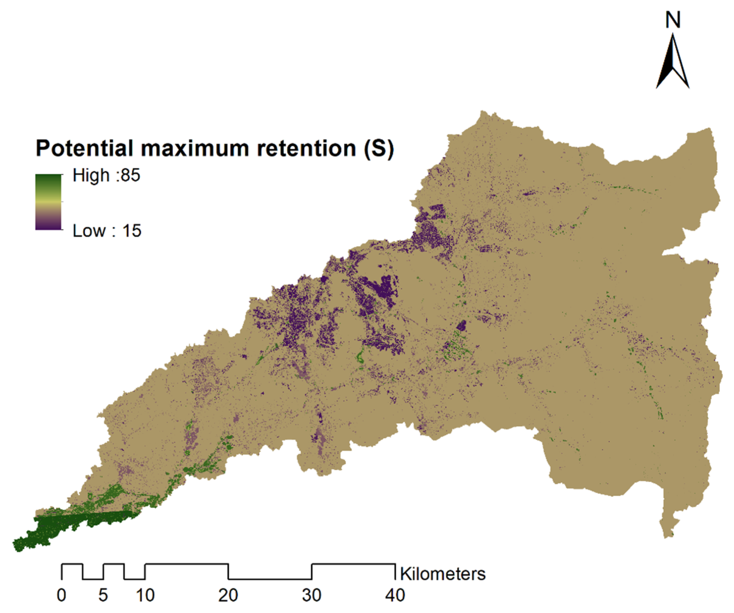
3.4. Potential Maximum Retention Map

Once the slope-adjusted CN_II map is generated, the potential maximum retention (S) is calculated in ArcGIS software using Equation (2) (Figure 12). As shown in Figure 12, the values of S range from 15 to 85 mm. The lowest S values within the basin are located in built-up areas, where the retention capacity is low. Similarly, bare areas located near municipalities had a poorer retention capacity as long as they are improperly used. On the other hand, agricultural areas have the highest S values as they have a high retention capacity. Noteworthy is that most of the study area is covered by the S values of 15–50 mm.

3.5. The Soil Conservation Service Runoff Map

The S and maximum daily rainfall maps were used as inputs in the GIS-based SCS-CN model to calculate the daily runoff. The resulting raster of runoff depth is displayed in Figure 13. A variation that ranges from 15 mm into a maximum of 47 mm was observed due to differences in topography and climate in the study area. The regions most exposed to surface runoff are built-up areas, where the CN frequently exceeds the value of 90. Furthermore, the mountainous area has a high runoff depth due to its land cover condition, steep slope, and soil type that has a high share of fine particles. As a result, the outflow can occur more easily in areas with these characteristics. On the other hand, the lowest values of the runoff occur in the southwestern part of the study area due to the high potential of water interception and water retention caused by vegetation coverage and loam soil texture type, respectively.

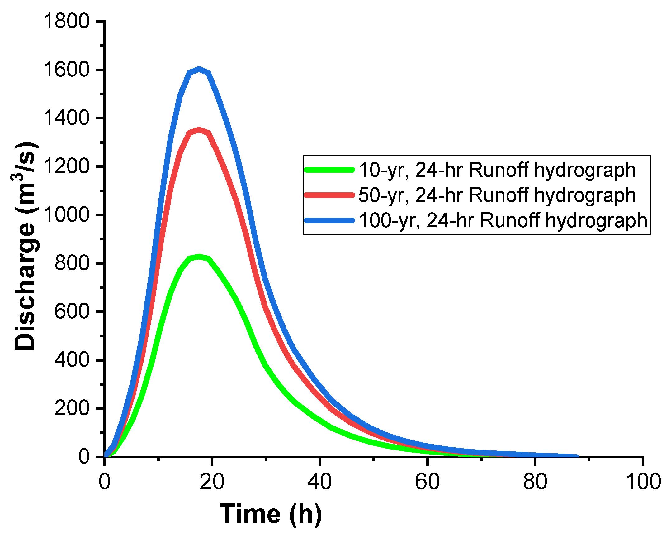
3.6. The Soil Conservation Service Storm Hydrograph

Design storm hydrographs for selected recurrence intervals (10, 50, and 100 years) were developed for the Wadi-Uranah basin (Figure 14). Figure 14 shows that the design frequency of the 10-years return period, a 24-h storm hydrograph, has a peak flow and peak time of 828 m³/s and 17.5 h, respectively. For 50 and 100 years, 24-h storm hydrographs, the peak flow and peak time were (1353 m³/s and 17.5 h) and (1603 m³/s and 17.5 h), respectively. These results are in agreement with Salami et al. [45] who concluded that the SCS method can be used for the development of peak storm hydrographs of different river return periods.

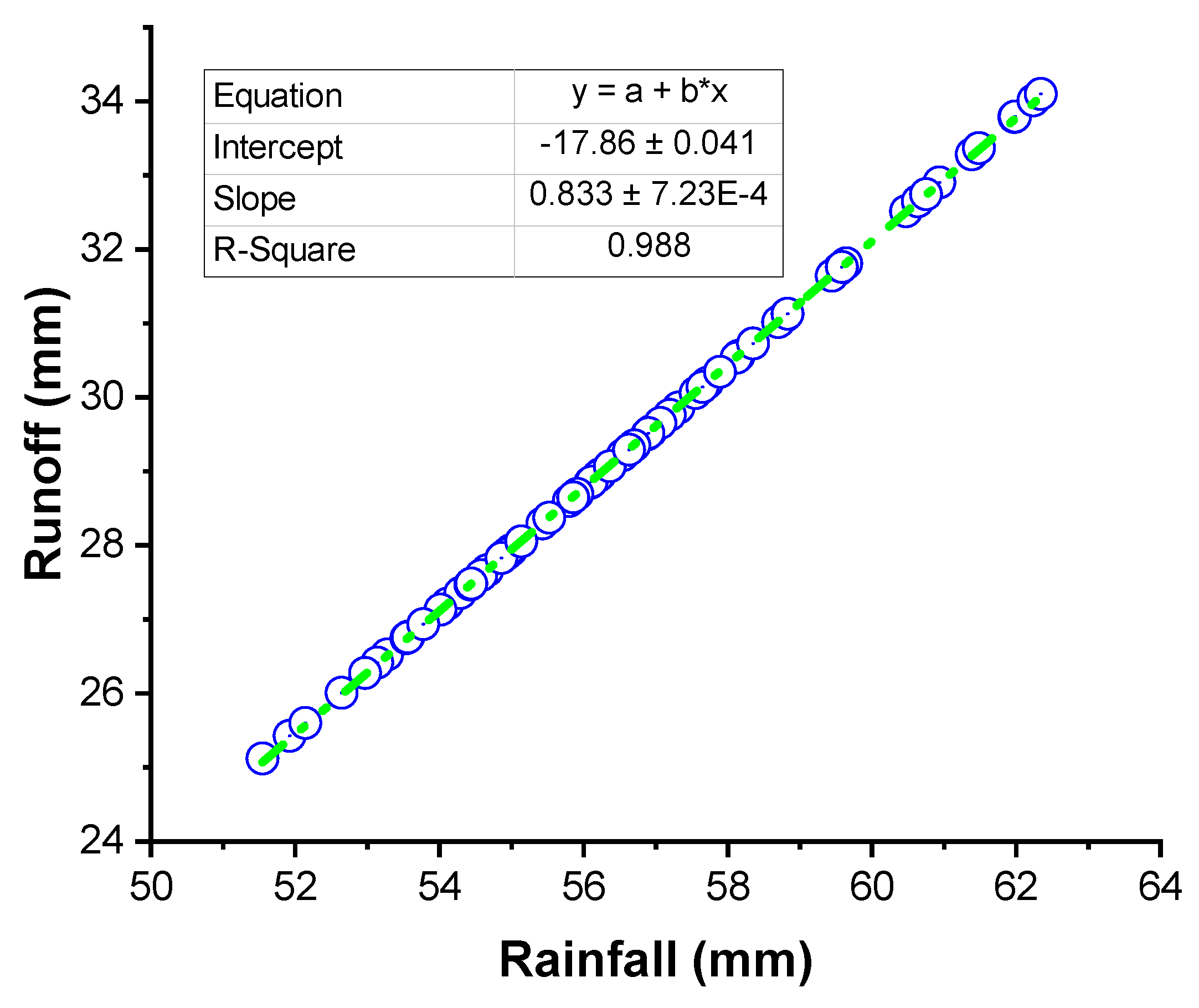
3.7. Rainfall-Runoff Correlation Analysis

The scatter-plot analysis shown in Figure 15 indicates a strong linear relationship between the maximum daily rainfall and SCS-CN runoff with a correlation coefficient of 0.98. This coefficient may provide valuable information on the extent of the basin response to runoff generation. Our study results are in line with the findings of Tirkey et al. [10] who found a good coefficient of determination (0.891) for a large study area using SCS-CN model. The slope of the trend line in the graph reflects the runoff coefficient, which is around 0.83. Such findings agreed with Peng and You [46] who came to the conclusion that the SCS-CN model has a better simulation effect on study areas with a coefficient of runoff greater than 0.5 than those with a coefficient of runoff less than 0.5.

4. Conclusions

The limited availability of measured surface runoff restricts various activities of water resources development and management. To overcome this limitation, the GIS, RS, and SCS-CN methods were combined to estimate the surface runoff in Wadi-Uranah basin, Saudi Arabia. The DEM, HSG, LULC, and daily precipitation records were used as inputs in the GIS-based SCS-CN model. Based on soil classification results, the study area was classified into two HSGs (B and C). The dominant HSG was group C, representing about 98.8% of the total area. Curve number values for the normal conditions (CN_II) ranged from 74 in the agricultural areas to 93 in the urban and rock areas. The CN_II values were further corrected using slope data to derive slope-adjusted CN_II (CN_IIα). The highest CN_IIα (95) was associated with a steep slope (>80%) of the study area, whilst the lowest CN_IIα (74) was found in the areas that have a slight slope (<20%). Furthermore, the study showed that the behavior of the runoff varies spatially depending on the LULC and the permeability of the soil. The peak runoff hydrograph flows obtained from SCS based dimensionless unit hydrograph for 10-, 50-, and 100-year return periods were 828, 1353, and 1603 m³/s, respectively. Therefore, SCS-CN method integrated with RS and GIS deserves further attention to study watershed characteristics in other basins in Saudi Arabia.

References

1. Deshmukh, D.S.; Chaube, U.C.; Hailu, A.E.; Gudeta, D.A.; Kassa, M.T. Estimation and comparision of curve numbers based on dynamic land use land cover change, observed rainfall-runoff data and land slope. J. Hydrol. 2013, 492, 89–101. [Google Scholar] [CrossRef]
2. Mishra, S.K.; Chaudhary, A.; Shrestha, R.K.; Pandey, A.; Lal, M. Experimental verification of the effect of slope and land use on SCS runoff curve number. Water Resour. Manag. 2014, 28, 3407–3416. [Google Scholar] [CrossRef]
3. Zade, M.; Ray, S.S.; Dutta, S.; Panigrahy, S. Analysis of runoff pattern for all major basins of India derived using remote sensing data. Curr. Sci. 2005, 88, 1301–1305. [Google Scholar]
4. USDA. Hydrology. In National Engineering Handbook; United States Department of Agriculture, Soil Conservation Service, US Government Printing Office: Washington, DC, USA, 1972. [Google Scholar]
5. Pradhan, R.; Pradhan, M.P.; Ghose, M.K.; Agarwal, V.S.; Agarwal, S. Estimation of RainfallRunoff using Remote Sensing and GIS in and around Singtam, East Sikkim. Int. J. Geomat. Geosci. 2010, 1, 466–476. [Google Scholar]
6. Shadeed, S.; Almasri, M. Application of GIS-based SCS-CN method in West Bank catchments, Palestine. Water Sci. Eng. 2010, 3, 1–13. [Google Scholar]
7. SCS. Urban Hydrology for Small Watersheds, Technical Release No. 55 (TR-55); United States Department of Agriculture, Soil Conservation Service, US Government Printing Office: Washington, DC, USA, 1986; pp. 2–6.
8. Chatterjee, C.; Jha, R.; Lohani, A.K.; Kumar, R.; Singh, R. Runoff curve number estimation for a basin using remote sensing and GIS. Asian Pac. Remote Sens. GIS J. 2001, 14, 1–7. [Google Scholar]
9. Bhuyan, S.J.; Mankin, K.R.; Koelliker, J.K. Watershed–scale AMC selection for hydrologic modeling. Trans. ASAE 2003, 46, 303. [Google Scholar] [CrossRef]
10. Tirkey, A.S.; Pandey, A.C.; Nathawat, M.S. Use of high-resolution satellite data, GIS and NRCS-CN technique for the estimation of rainfall-induced run-off in small catchment of Jharkhand India. Geocarto. Int. 2014, 29, 778–791. [Google Scholar] [CrossRef]
11. Liu, X.; Li, J. Application of SCS model in estimation of runoff from small watershed in Loess Plateau of China. Chin. Geogr. Sci. 2008, 18, 1235–1241. [Google Scholar] [CrossRef]
12. Topno, A.; Singh, A.K.; Vaishya, R.C. SCS-CN Runoff estimation for Vindhyachal region using remote sensing and GIS. Int. J. Adv. Remote Sens. GIS 2015, 4, 1214–1223. [Google Scholar] [CrossRef]
13. Huang, M.; Gallichand, J.; Wang, Z.; Goulet, M. A modification to the Soil Conservation Service curve number method for steep slopes in the Loess Plateau of China. Hydrol. Process. 2006, 20, 579–589. [Google Scholar] [CrossRef]
14. Hawkins, R.H.; Ward, T.; Woodward, D.E.; Van Mullem, J. Curve Number Hydrology: State of the Practice Reston; ASCE: Washington, DC, USA, 2009; p. 106. [Google Scholar]
15. Shi, W.; Huang, M.; Gongadze, K.; Wu, L. A modified SCS-CN method incorporating storm duration and antecedent soil moisture estimation for runoff prediction. Water Resour. Manag. 2017, 31, 1713–1727. [Google Scholar] [CrossRef]
16. Fisher, P.F.; Comber, A.J.; Wadsworth, R. Land use and land cover: Contradiction or complement. In Re-Presenting GIS; Wiley: Hoboken, NJ, USA, 2005; pp. 85–98. [Google Scholar]
17. NRCS. Hydrologic Soil Groups. In National Engineering Handbook; United States Department of Agriculture, Natural Resources Conservation Science, US Government Printing Office: Washington, DC, USA, 2009. [Google Scholar]
18. Chaplot, V.A.; Le Bissonnais, Y. Runoff features for interrill erosion at different rainfall intensities, slope lengths, and gradients in an agricultural loessial hillslope. Soil. Sci. Soc. Am. J. 2003, 67, 844–851. [Google Scholar] [CrossRef]
19. Philip, J.R. Hillslope infiltration: Planar slopes. Water Resour. Res. 1991, 27, 109–117. [Google Scholar] [CrossRef]
20. Evett, S.R.; Dutt, G.R. Length and slope effects on runoff from sodium dispersed, compacted earth microcatchments. Soil. Sci. Soc. Am. J. 1985, 49, 734–738. [Google Scholar] [CrossRef]
21. Fang, H.Y.; Cai, Q.G.; Chen, H.; Li, Q.Y. Effect of rainfall regime and slope on runoff in a gullied loess region on the Loess Plateau in China. Environ. Manag. 2008, 42, 402–411. [Google Scholar] [CrossRef]
22. Chaudhary, A.; Mishra, S.K.; Pandey, A. Experimental verification of effect of slope on runoff and curve numbers. J. Indian Water Res. Soc. 2013, 33, 40–46. [Google Scholar]
23. Jha, R.K.; Mishra, S.K.; Pandey, A. Experimental verification of effect of slope, soil, and AMC of a fallow land on runoff curve number. J. Indian Water Res. Soc. 2014, 34, 40–47. [Google Scholar]
24. Cheng, Q.; Ko, C.; Yuan, Y.; Ge, Y.; Zhang, S. GIS modeling for predicting river runoff volume in ungauged drainages in the Greater Toronto Area, Canada. Comput. Geosci. 2006, 32, 1108–1119. [Google Scholar] [CrossRef]
25. Zhan, X.; Huang, M.L. ArcCN-Runoff: An ArcGIS tool for generating curve number and runoff maps. Environ. Modell. Softw. 2004, 19, 875–879. [Google Scholar] [CrossRef]
26. Nayak, T.R.; Jaiswal, R.K. Rainfall-runoff modelling using satellite data and GIS for Bebas river in Madhya Pradesh. J. Inst. Eng. India 2003, 84, 47–50. [Google Scholar]
27. Geena, G.B.; Ballukraya, P.N. Estimation of runoff for Red hills watershed using SCS method and GIS. Indian J. Sci. Technol. 2011, 4, 899–902. [Google Scholar]
28. Gitika, T.; Ranjan, S. Estimation of surface runoff using NRCS curve number procedure in Buriganga Watershed, Assam, India-a geospatial approach. Int. Res. J. Earth Sci. 2014, 2, 1–7. [Google Scholar]
29. Al Saud, M. Morphometric analysis of Wadi Aurnah drainage system, western Arabian Peninsula. Open Hydrol. J. 2009, 3, 1–10. [Google Scholar]
30. Dawod, G.M.; Mirza, M.N.; Al-Ghamdi, K.A. GIS-based estimation of flood hazard impacts on road network in Makkah city, Saudi Arabia. Environ. Earth Sci. 2012, 67, 2205–2215. [Google Scholar] [CrossRef]
31. Saxton, K.E.; Rawls, W.; Romberger, J.S.; Papendick, R.I. Estimating generalized soil-water characteristics from texture. Soil. Sci. Soc. Am. J. 1986, 50, 1031–1036. [Google Scholar] [CrossRef]
32. Cosby, B.J.; Hornberger, G.M.; Clapp, R.B.; Ginn, T. A statistical exploration of the relationships of soil moisture characteristics to the physical properties of soils. Water Resour. Res. 1984, 20, 682–690. [Google Scholar] [CrossRef] [Green Version]
33. Wang, X.; Liu, T.; Yang, W. Development of a robust runoff-prediction model by fusing the rational equation and a modified SCS-CN method. Hydrolog. Sci. J. 2012, 57, 1118–1140. [Google Scholar] [CrossRef] [Green Version]
34. Mishra, S.K.; Singh, V.P. Another look at SCS-CN method. J. Hydrol. Eng. 1999, 4, 257–264. [Google Scholar] [CrossRef]
35. NRCS. Estimation of Direct Runoff from Storm Rainfall. In National Engineering Handbook; United States Department of Agriculture, Natural Resources Conservation Science, US Government Printing Office: Washington, DC, USA, 2004. [Google Scholar]
36. Hawkins, R.H.; Hjelmfelt, A.T., Jr.; Zevenbergen, A.W. Runoff probability, storm depth, and curve numbers. J. Irrig. Drain. E ASCE 1985, 111, 330–340. [Google Scholar] [CrossRef]
37. McCuen, R.H. A Guide to Hydrologic Analysis Using SCS Methods; Prentice-Hall, Inc.: Englewood Cliffs, NJ, USA, 1982; p. 145. [Google Scholar]
38. Sherman, L.K. Streamflow from rainfall by the unit-graph method. Eng. News Rec. 1932, 108, 501–505. [Google Scholar]
39. SCS. Use of Storm and Watershed Characteristics in Synthetic Hydrograph Analysis and Application; United States Department of Agriculture, Soil Conservation Service, US Government Printing Office: Washington, DC, USA, 1957.
40. Singh, V.P.; Corradini, C.; Melone, F. A comparison of some methods of deriving the instantaneous unit hydrograph. Hydrol. Res. 1985, 16, 1–10. [Google Scholar] [CrossRef]
41. NRCS. Ponds: Planning, Design, Construction. In Agriculture Handbook No. 590; United States Department of Agriculture, Natural Resources Conservation Science, US Government Printing Office: Washington, DC, USA, 1997. [Google Scholar]
42. Subyani, A.M.; Al-Amri, N.S. IDF curves and daily rainfall generation for Al-Madinah city, western Saudi Arabia. Arab. J. Geosci. 2015, 8, 11107–11119. [Google Scholar] [CrossRef]
43. Viessman, W., Jr.; Lewis, G.L. Introduction to Hydrology; HarperCollins College Publishers: New York, NY, USA, 1996. [Google Scholar]
44. Zhao, W.W.; Fu, B.J.; Chen, L.D.; Zhang, Q.J.; Zhang, Y.H. Effects of land-use pattern change on rainfall-runoff and runoff-sediment relations: A case study in Zichang watershed of the Loess Plateau of China. J. Environ. Sci. 2004, 16, 436–442. [Google Scholar]
45. Salami, A.W.; Bilewu, S.O.; Ayanshila, A.M.; Oritola, S.F. Evaluation of synthetic unit hydrograph methods for the development of design storm hydrographs for Rivers in South-West, Nigeria. J. Am. Sci. 2009, 5, 23–32. [Google Scholar]
46. Peng, D.Z.; You, J.J. Application of modified SCS model into runoff simulation. J. Water Res. Water Eng. 2006, 17, 20–24. [Google Scholar]
Figure 1. (A) Location map of Wadi-Uranah basin in Saudi Arabia, (B) a magnified view of the study site.
Water 12 01924 g001
Figure 2. Extraction of drainage network for the study region (Wadi-Uranah). (A) Digital elevation model map of the study area; (B) triangular irregular networks map of the study area; (C) flow direction map of the study area; (D) stream order map of the study area.
Water 12 01924 g002
Figure 3. Flowchart showing the methodology employed by the geographic information system (GIS) based soil conservation service-curve number (SCS-CN) model in estimating the surface runoff.
Water 12 01924 g003
Figure 4. Soil textural class map of the study area.
Water 12 01924 g004
Figure 5. Hydrologic soil group (HSG) map of the study area.
Water 12 01924 g005
Figure 6. (A) Slope map of the study area, (B) aspect map of the study area.
Water 12 01924 g006
Figure 7. Maximum daily precipitation distribution map of the study area.
Water 12 01924 g007
Figure 8. Land use/land cover (LULC) map of the study area.
Water 12 01924 g008
Figure 9. Curve number (CNII) associated with AMC-II for each cell of the study area.
Water 12 01924 g009
Figure 10. (A) Curve number (CNI) associated with AMC-I for each cell of the study area, (B) curve number (CNIII) associated with AMC-III for each cell of the study area.
Water 12 01924 g010
Figure 11. Slope-adjusted CNII map for each cell of the study area.
Water 12 01924 g011
Figure 12. Potential maximum retention (S) map of the study area.
Water 12 01924 g012
Figure 13. Potential runoff map of the study area.
Water 12 01924 g013
Figure 14. The Soil Conservation Service storm hydrograph of different return periods for the study area.
Water 12 01924 g014
Figure 15. The rainfall and SCS-CN runoff relationship for the study area.
Water 12 01924 g015