Article

Spatial Predictions of Debris Flow Susceptibility Mapping Using Convolutional Neural Networks in Jilin Province, China

College of Construction Engineering, Jilin University, Changchun 130026, China
*
Author to whom correspondence should be addressed.
Water 2020, 12(8), 2079; https://doi.org/10.3390/w12082079
Submission received: 18 June 2020 / Revised: 16 July 2020 / Accepted: 20 July 2020 / Published: 22 July 2020

Abstract

:
Debris flows are a major geological disaster that can seriously threaten human life and physical infrastructures. The main contribution of this paper is the establishment of two–dimensional convolutional neural networks (2D–CNN) models by using SAME padding (S–CNN) and VALID padding (V–CNN) and comparing them with support vector machine (SVM) and artificial neural network (ANN) models, respectively, to predict the spatial probability of debris flows in Jilin Province, China. First, the dataset is randomly divided into a training set (70%) and a validation set (30%), and thirteen influencing factors are selected to build the models. Then, multicollinearity analysis and gain ratio methods are used to quantify the predictive ability of factors. Finally, the area under the receiver operatic characteristic curve (AUC) and statistical methods are utilized to measure the accuracy of the models. The results show that the S–CNN model gets the highest AUC value of 0.901 in the validation set, followed by the SVM model, the V–CNN model, and the ANN model. Three statistical methods also show that the S–CNN model produces minimum errors compared with other models. The S–CNN model is hailed as an important means to improve the accuracy of debris–flow susceptibility mapping and provides a reasonable scientific basis for critical decisions.

1. Introduction

Debris flows are defined as large–scale movements of a mixture of soil, rock, and water from the top to the bottom of the mountains. Debris flows cause numerous casualties and a great amount of property damage each year [1,2]. In the past few decades, the formation and movement mechanism of debris flows have been the focus of research on geological disasters [3,4]. The occurrence of a debris flow is sudden and destructive and is usually affected by factors such as earthquakes, heavy rainfall, and human activities. Therefore, it is difficult to accurately predict the spatial distribution of debris flows and areas of susceptibility [5].
Debris flow susceptibility refers to the probability of debris flow occurring in a given area [6]. For the sake of decreasing the hazards caused by debris flows, debris flow susceptibility mapping (DFSM) is a direct and effective method, which is a basic means to discover relationships between debris flows and influencing factors and identify potential debris flow areas. The combined action of many influencing factors leads to the occurrence of a debris flow. Therefore, using these influencing factors to predict the debris flow susceptibility spatial distribution is essential in preventing and decreasing a debris flow’s damages. At present, various methods are being utilized to produce debris flow susceptibility maps [7,8]. These methods can be divided into three categories: qualitative methods, traditional statistical methods, and machine learning (ML) methods. Qualitative methods mainly include the analytic hierarchy process (AHP) [9,10,11], fuzzy logic method [12,13,14], etc. These kinds of methods mainly rely on the experience of experts, and the evaluation results have strong subjectivity. Traditional statistical methods mainly include the weight of evidence [15], frequency ratio [16], statistical index (SI) [17], and so on. These methods are not sufficient for data mining [18,19]. Therefore, more effective methods are urgently needed to improve the quality of debris–flow susceptibility maps.
With the rapid development of artificial intelligence in recent years, ML methods have been widely employed in regional debris flows prediction, including support vector machine (SVM) [20,21,22], Naïve Bayes (NB) [23], artificial neural network (ANN) [24,25], random forest (RF) [26,27], boosted regression tree(BRT) [28], logistic regression(LR) [29], etc. Compared with traditional statistical methods, ML methods are more suitable for finding the data relationships between debris flows and influencing factors [18]. But with the deepening of the research, we can find that traditional ML methods directly classify the debris flow data and ignore the relationships existing in the data, which ultimately fails to further improve the classification accuracy [30]. Therefore, using traditional ML methods to evaluate debris flows does not satisfy the needs in Jilin Province, China, where debris flows cause many casualties and high economic losses every year, especially during the rainy season [31,32].
To settle this problem, deep learning (DL), as an important branch of ML methods, has been supported and embraced by scholars as soon as it emerged because it can complete the target problems better than traditional ML methods [33]. DL algorithms mainly include convolutional neural network (CNN), recurrent neural network (RNN), generative adversarial network (GAN), etc. Among these, CNN is one of the most popular DL algorithms and has been gradually applied to DFSM [34,35]. Compared with traditional ML algorithms, the CNN structure adds the convolution layers and subsampling layers. Hence, CNN has fewer parameters and allows easier mining of the latent relationships that are hidden in the data. Specifically, it has outstanding ability in image classification because of its use of the convolution layers and subsampling layers, which can effectively extract the latent features of an image [36,37]. Moreover, there are two data processing methods applied when performing convolution and subsampling operations: SAME padding and VALID padding. SAME padding could ensure the integrity of the data when processing the data. However, VALID padding would discard data at the edge of the matrix for a quick calculation, resulting in an imbalanced use of the edge data and the central data. Wang et al. [30] used VALID padding to process debris flow data and generated a highly accurate debris flow susceptibility map. In this paper, the S–CNN and V–CNN models are established by using SAME padding and VALID padding to research the spatial distribution of debris–flow susceptibility in Jilin Province, China.
The purpose of this study is to provide a CNN framework for regional debris flow susceptibility evaluation in Jilin Province, China. The two primary contributions of this paper can be summarized as follows. First, we are attempting to select a CNN model with more predictive ability to provide valuable information for further research. Second, a comparison of the S–CNN, SVM, V–CNN, and ANN models is proposed for the spatial prediction of debris–flow susceptibility. To measure the model’s accuracy, the receiver operatic characteristic (ROC) curve, the accuracy (ACC), F–measure, and the mean absolute error (MAE) are utilized for comparison. More importantly, it is hoped that the research from this paper can provide a more solid decision basis for policymakers to reduce the harm caused by debris flow.

2. Study Area

Jilin Province is located in the part of northeast China, extending between 40°50′ N and 46°19′ N latitude and 121°38′ E and 131°19′ E longitude with an area of 187,400 km2, as shown in Figure 1.
The study area has a temperate continental monsoon climate. The average temperature in winter is below −11 °C. The annual temperature difference is 35 °C to 42 °C, and the daily temperature difference is generally 10 °C to 14 °C. The average annual precipitation is 400 mm to 600 mm, but the seasonal and regional differences are large and the eastern part has the most abundant rainfall. There are many lakes in Jilin Province, and the western plains are mostly natural lakes, such as the Moon Bubble; the eastern mountainous areas are mainly artificial lakes and volcanic lakes, such as the Triangle Dragon Bay.
The geomorphologic difference in Jilin Province is obvious. The terrain is inclined from the southeast to the northwest, showing obvious characteristics of southeast high elevation and northwest low elevation. With the central Big Black Mountain as the boundary, the landforms can be divided into the eastern mountains, the central, and the western plains. The geomorphology includes weathered, eroded, and denuded volcanic landforms with alluvial fans and fluvial river systems. In Jilin Province, the main geology and lithology are shown in Table 1.
All in all, the geological environmental conditions are exceedingly complex, so many influencing factors can cause debris flows to occur in Jilin Province. During the rainy season, debris flows occur more frequently, causing high economic losses every year. Therefore, policymakers urgently need more accurate and reliable debris flow susceptibility maps to provide more reasonable preventive measures for the local area.

3. Materials and Methods

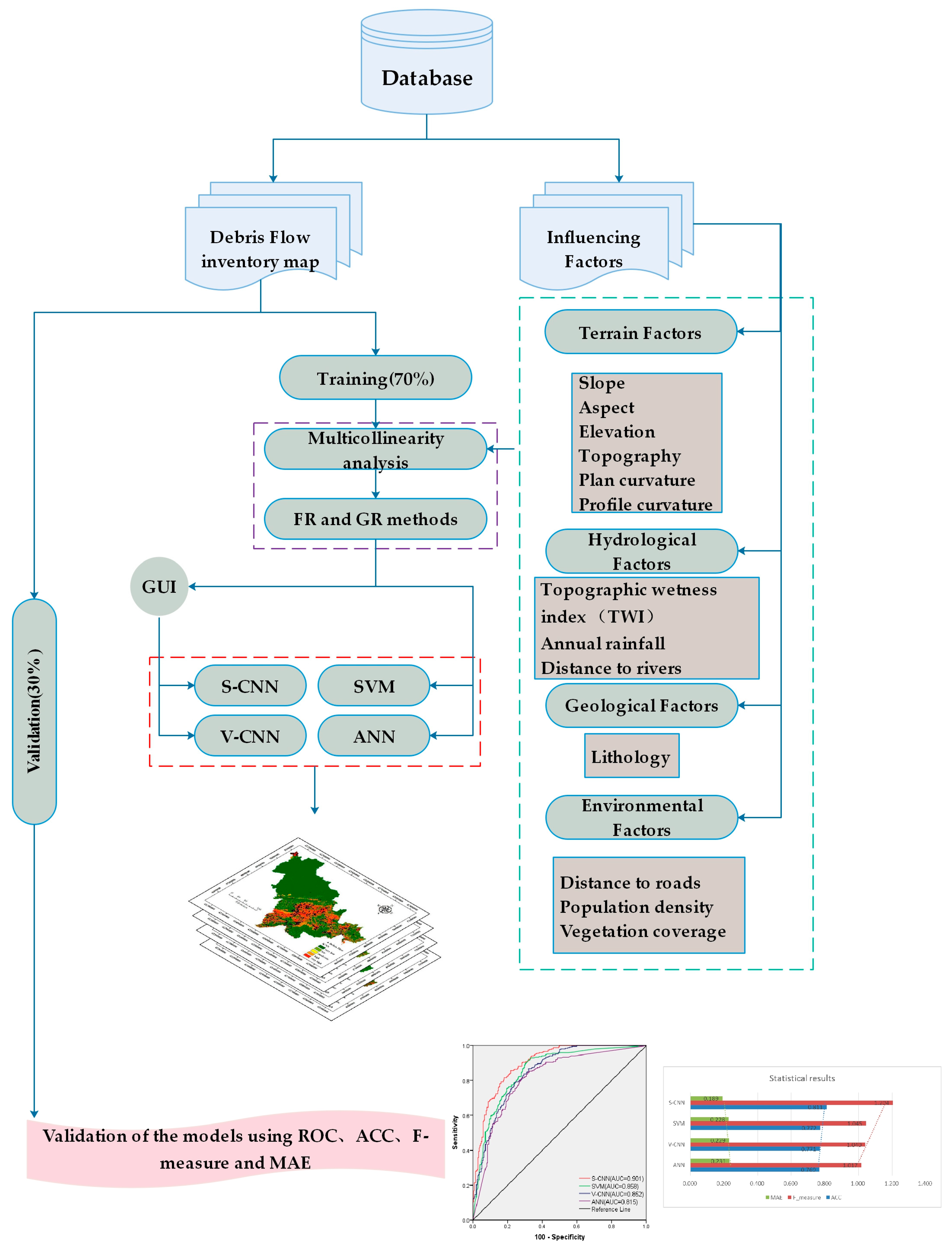
In this paper, the following four steps were used to complete the spatial prediction of debris–flow susceptibility in the study area. (1) Data preparation and selection of influencing factors. (2) Influencing factors analysis using Multicollinearity analysis, the frequency ratio (FR) method, and gain ratio (GR) method. (3) Establishment of models based on S–CNN, SVM, V–CNN, and ANN algorithms. (4) Models evaluations by using multiple evaluation indicators including the ROC curve, ACC, F–measure, and MAE. A flowchart is shown in Figure 2.

3.1. Data Preparation

The quality of a debris flow inventory map is vital and ultimately affects the evaluation results of the study area [38,39]. Therefore, a quality–assured data source will help to uncover potential relationships between the occurrence of debris flows and influencing factors. In this paper, a debris flow inventory map has been prepared from different sources, including field investigation, remote sensing interpretation, and official data. 868 debris flow locations and 868 non–debris flow locations were randomly selected in the debris flow and non–debris flow areas. The dataset was randomly split into a training set (70%) to train the models and a validation set (30%) to check the accuracy of the models, in which debris flow and non–debris flow locations were equally balanced. Figure 1 shows the specific location distribution of debris flow in Jilin Province, China.
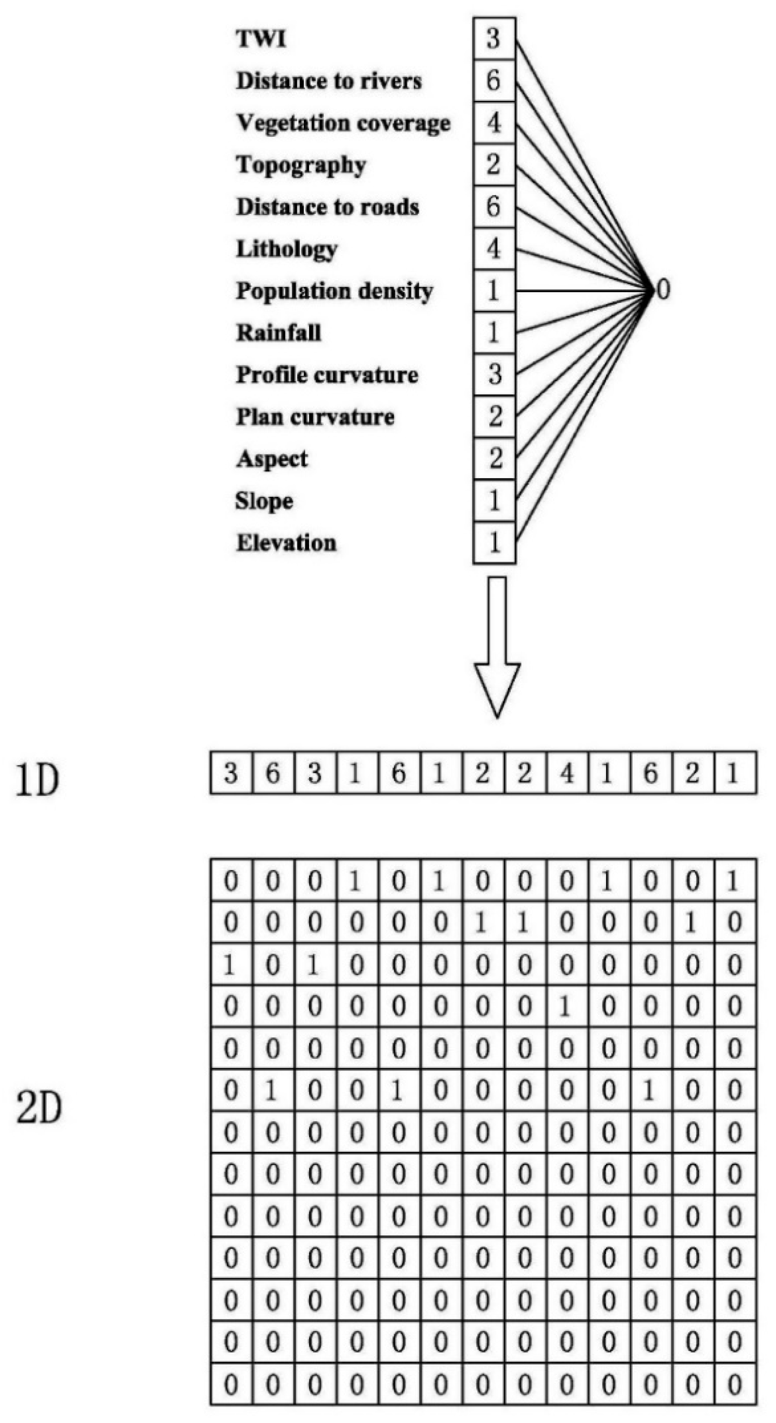
In ML algorithms, data can be read directly in text or table format. However, input data needs to be converted to matrices to feed to CNN. In this paper, thirteen influencing factors were used, so each grid cell had thirteen corresponding values. In a binary classification problem, 0 is usually used to represent non–debris flow location and 1 is used to represent debris flow location. Then some grid cells’ influencing factors values are shown in Figure 3.
In this paper, 2D–CNN was utilized to build the models. The conversion process of 1D to 2D is shown in Figure 4. Finally, the CNN data preparation was implemented by using a python–based graphical user interface (GUI).

3.2. Influencing Factors

Selecting high quality influencing factors is a crucial step in producing debris flow susceptibility maps because irrelevant factors or noise factors can damage the quality of the models and thus reduce the quality of DFSM. Unfortunately, there is not presently an accepted benchmark for the selection of debris flow influencing factors. Therefore, based on previous researches and experts experience [40], a total of thirteen influencing factors were selected, including elevation, slope, aspect, plan curvature, profile curvature, topographic wetness index (TWI), distance to roads, distance to rivers, lithology, population density, annual rainfall, topography, and vegetation coverage. The digital elevation model (DEM) was downloaded from Google Maps with a spatial resolution of 100 m. To improve the quality of DFSM, grid cells were used in this paper which are recognized by the majority of researchers. The database for influencing factors is shown in Table 2.
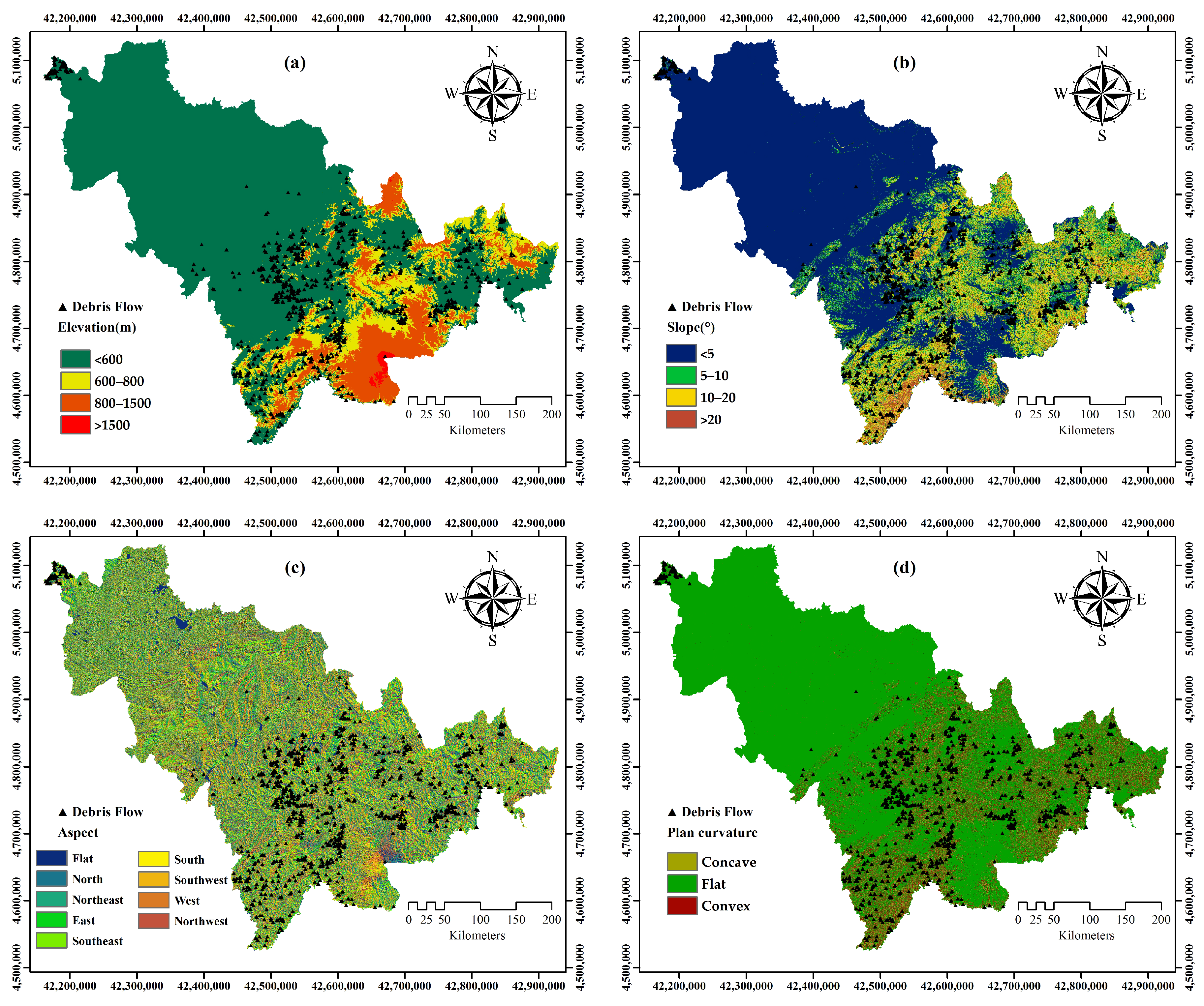
Elevation is a critical and widely used factor for DFSM [41,42,43]. Debris flows are also closely correlated with rainfall, vegetation cover, geologic bedrock, soil composition, and river discharge which vary at different altitudes. The altitude of Changbai Mountain is 800–1500 m which is located in the southeast of the research area. The main peak of Changbai Mountain and its surrounding peaks are over 2000 m, and the central plain is 600–800 m. Therefore, elevation was classified into four classes: <600 m, 600–800 m, 800–1500 m, and >1500 m (Figure 5a).
Slope is also a factor frequently used in DFSM [44]. Slope affects the shear strength, and runoff of the slope is closely related to the occurrence of debris flows [45]. In the northwest plain of Jilin Province, the slope is mainly 0–5°, while in the southeast mountainous area, the slope is usually 10°, with a few areas exceeding 20°. In this paper, slope was classified into four classes: 0–5°, 5–10°, 10–20°, and >20° (Figure 5b).
Aspect refers to the downslope direction. Aspect is affected by rainfall, duration of sunshine, wind direction, and weathering such as frost action [46,47]. These factors all play key roles in the occurrence of debris flows. Aspect was classified into nine classes: flat, north, northeast, east, southeast, south, southwest, west, and northwest (Figure 5c).
Plan curvature delineates the morphology of the topography and represents the ability of water divergence or convergence to affect the occurrence of debris flows [48,49]. Plan curvature was divided into three classes: concave, flat, and convex (Figure 5d).
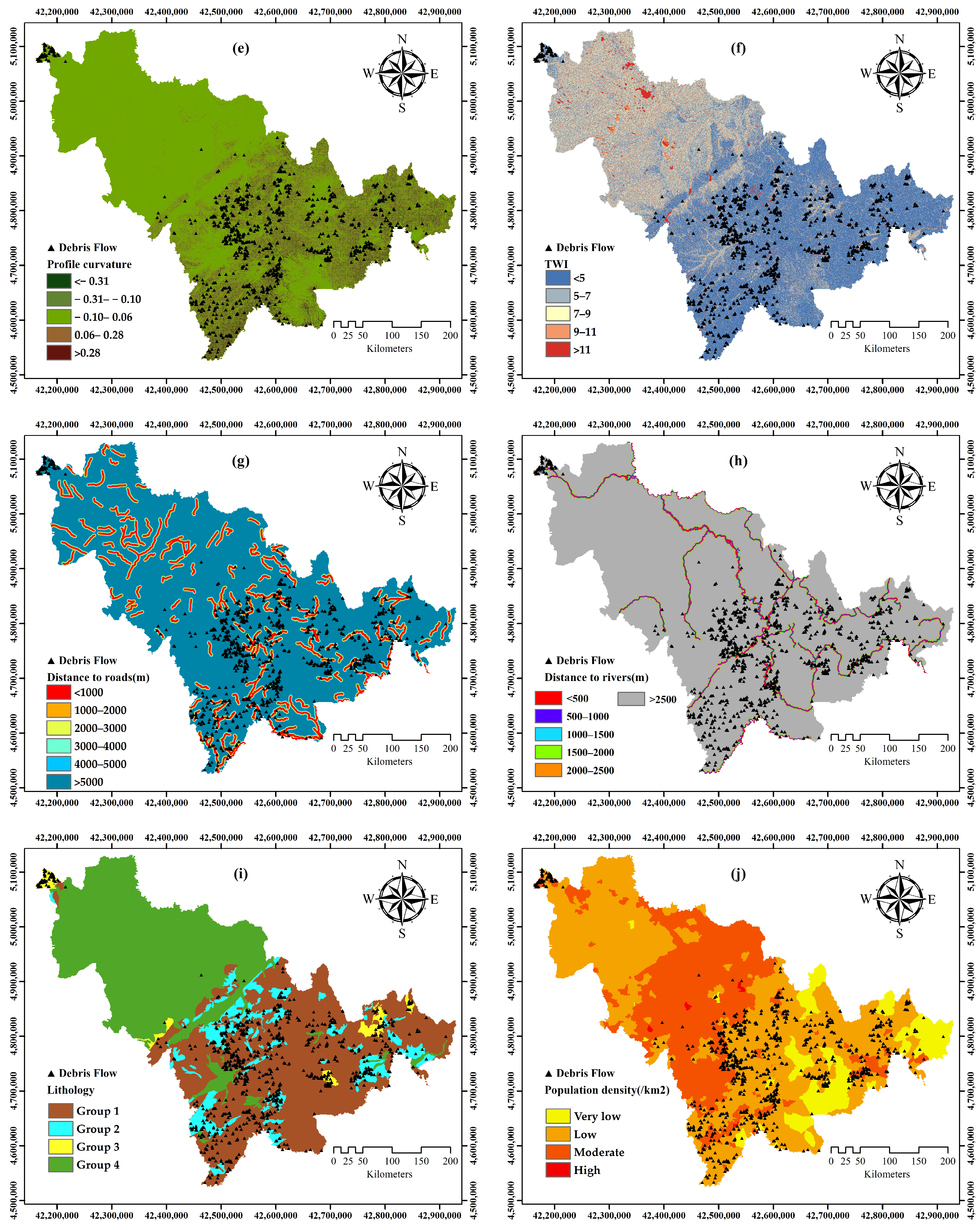
Profile curvature reflects the rate at which the aspect changes and affects the size of the catchment area, which is closely related to debris flow scales [50]. Profile curvature was classified into five classes by natural breaks method: <−0.31, −0.31–−0.10, −0.10–0.06, 0.06–0.28, and 0.28–2.10 (Figure 5e).
TWI is also a significant factor for DFSM [51]. The higher the TWI value, the easier it is for soil moisture to reach saturation, and the probability of debris flow occurring is increased. Most debris flows in Jilin Province occurred in areas with TWI less than 5. For the sake of a comprehensive analysis, TWI was classified into five classes using an interval of 2: <5, 5–7, 7–9, 9–11, and >11 (Figure 5f).
Distance to roads refers to the distance from the debris flow locations to a road. In general, the closer a debris flow location is to a road, the more lives and property of pedestrians are threatened. Additionally, debris flows are more likely to occur on slopes that are close to the roads because of human interference and so this is also a very important factor. Considering the reasonableness of the buffer distance in the study area, distance to roads was classified into six classes at 1000 m intervals: <1000 m, 1000–2000 m, 2000–3000 m, 3000–4000 m, 4000–5000 m, and >5000 m (Figure 5g).
Distance to the rivers can affect the hydrologic index of the slope and thus the slope stability. Slopes are more prone to debris flows which are closer to rivers because the distance describes the erosion power of streams [52]. Considering the influence of rivers on slope stability, distance to rivers was classified into six classes with intervals of 500 m: <500 m, 500–1000 m, 1000–1500 m, 1500–2000 m, 2000–2500 m, and >2500 m (Figure 5h).
Bedrock is a key factor with respect to the degree of weathering, mineral composition rock type, the orientation of discontinuities such as bedding, fractures, foliations with respect to slope direction (aspect). Rocks with phyllosilicate minerals are particularly prone to mass wasting such as claystones, shales, mudstones, tuffs, pyroclastic rocks, slate, and phyllite. Rocks with discontinuities inclined in the same direction as topographic slope are highly prone to mass wasting. The research area encompasses 370 lithostratigraphic units. Segoni et al. [53] have proposed several classification methods in complex geological settings. In the paper, we attached great importance to the anti–weathering ability of rocks. Debris flows are more likely to occur where the lithology is easily weathered, which is because the weathering crust is easily eroded under the action of external forces. For example, the slope composed of loose rock and soil will lead to debris flows with unpredictable consequences [54,55]. According to the anti–weathering ability of rocks, the lithology was classified into four classes: group 1 (granite, basalt, carbonate rock, gneiss, etc.), group 2 (glutenite, slate, phyllite, schist, etc.), group 3 (claystones, pyroclastic rock, etc.), and group 4 (soil) (Figure 5i).
Population density is a key factor for debris flow occurring. Human engineering activities can change the shape of slopes, vegetation cover, etc., which could provide sufficient conditions for debris flows [56]. According to the number of people per square kilometers, the population density was classified into four classes: very low (0–10), low (10–100), moderate (100–500), and high (>500) (Figure 5j).
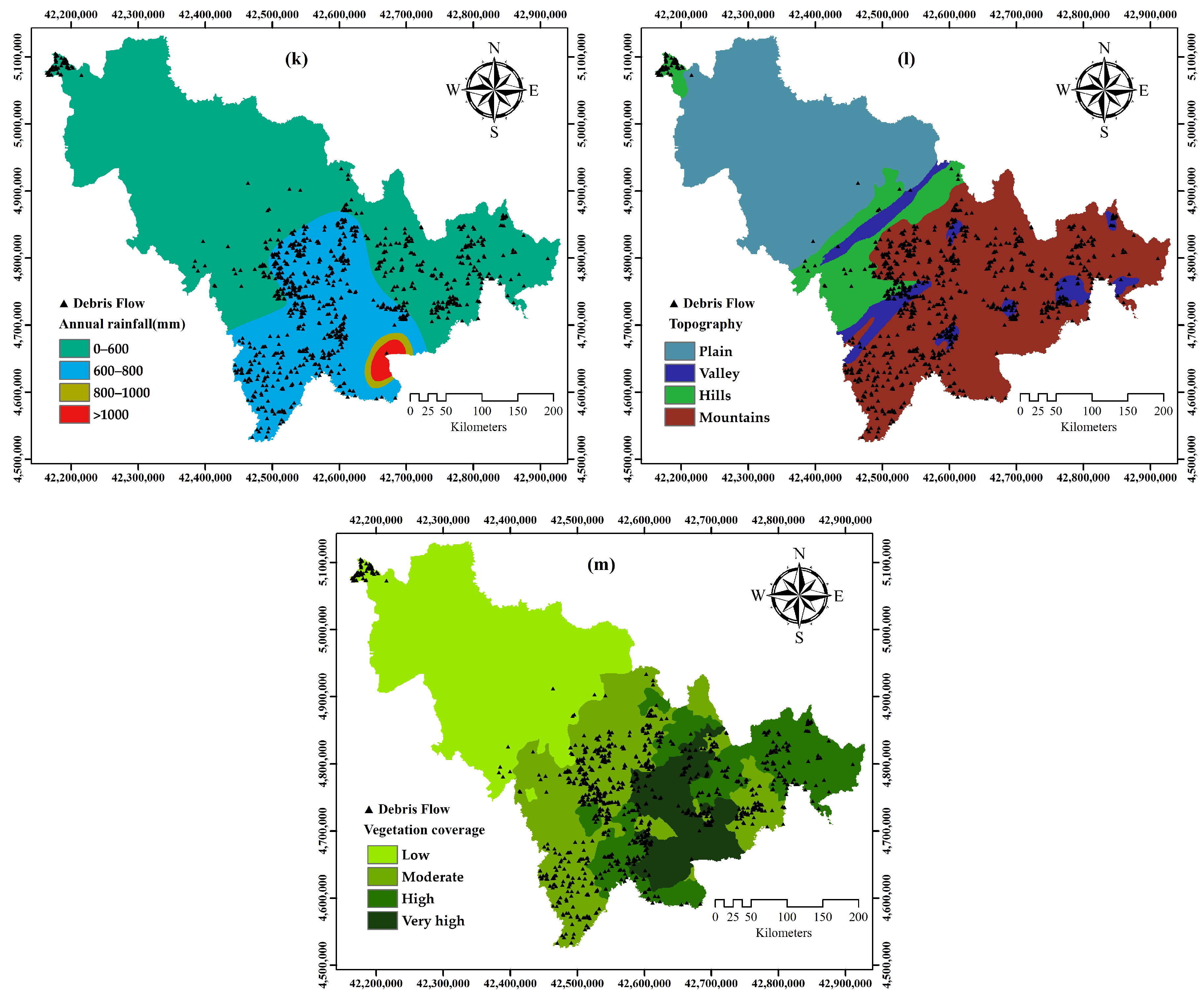
It is well known that most debris flows occur during the rainy season [57]. Because the continuous heavy rainfall increases the runoff and seepage flow, the possibility of debris flow occurring is greatly increased. According to the annual rainfall distribution in the study area, annual rainfall was classified into four classes: 0–600 mm, 600–800 mm, 800–1000 mm, and >1000 mm (Figure 5k).
Topography affects the size, formation, and movement of debris flows [58]. Based on existing studies and topography in Jilin Province, topography was classified into four classes: plain, valley, hills, and mountains (Figure 5l).
The level of vegetation coverage represents the growth status of vegetation in an area. Generally, the better the vegetation growth, the less prone an area is to debris flow. In Jilin Province, vegetation coverage of northwestern plain is less than 20%, while that of Changbai Mountain is more than 80%. The vegetation coverage in the central region is mainly 20% to 50%. Therefore, vegetation coverage was classified into four classes: low (<20%), moderate (20–50%), high (50–80%), and very high (>80%) (Figure 5m).

3.3. Evaluation of Influencing Factors

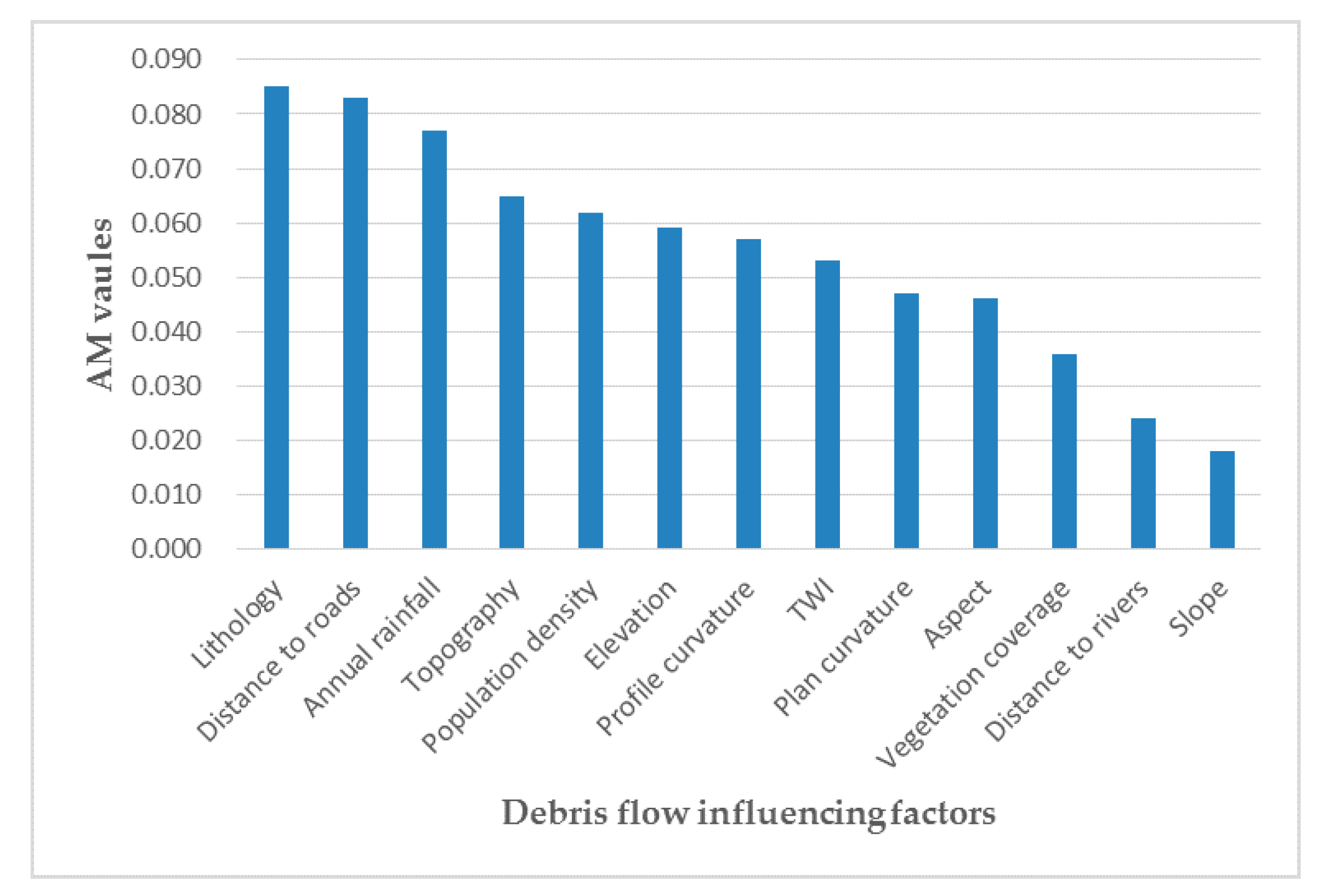
In the paper, thirteen influencing factors were selected through reference to previous research literature and expert experiences. Specifically, multicollinearity analysis was used to detect the collinearity between factors, and the FR method was utilized to ascertain the spatial relationship between each influencing factor and debris flows [59,60]. In addition, we used the GR method to quantify the predictive ability of the factors and exclude irrelevant factors.

3.3.1. Multicollinearity Analysis

Collinearity means that the influencing factors are not independent of each other, a situation that can damage a model’s quality [61]. Therefore, to improve the quality of DFSM, strong collinear factors must be discarded. Then tolerance and variance inflation factor (VIF) methods were used in the paper to quantify the collinearity between the factors. When the tolerance value is less than 0.1 or the VIF value is greater than 10, we assume that the collinearity of the factor satisfies the requirements. The formulas for calculating tolerance and VIF are as follows [62]:
T o l e r a n c e = 1 R j 2
V I F = [ 1 T o l e r a n c e ]
where is the coefficient of determination for the regression of the explanatory variable j on all the other explanatory variables.

3.3.2. Frequency Ratio Method

FR method is a geospatial assessment tool that can quantify the relationship between the influencing factors and debris flows [63]. This method uses the number of pixels dominating a particular area of a region and the number of pixels affected by a debris flow. In general, the slide ratio and the class ratio were utilized to calculate the FR value. In the relationship analysis, 1 is deemed to be the average value. When the FR value is greater than 1, it represents a higher connection between influencing factors and a debris flow. The formulas for calculating the FR value are as follows:
F R   v a l u e = S l i d e   r a t i o C l a s s   r a t i o
S l i d e   r a t i o = N u m b e r   o f   d e b r i s   f l o w   p i x e l s   i n   a   p a r t i c u l a r   c l a s s T o t a l   n u m b e r   o f   d e b r i s   f l o w   p i x e l s
C l a s s   r a t i o = N u m b e r   o f p i x e l s   i n   a   p a r t i c u l a r   c l a s s T o t a l   n u m b e r   o f p i x e l s

3.3.3. Gain Ratio Method

In the study area, the predictive ability of influencing factors is not the same. Some influencing factors may cause errors in the models and reduce the quality of debris–flow susceptibility maps. Therefore, it is necessary to evaluate the importance of influencing factors. In this study, the GR method was introduced to measure the predictive ability of influencing factors [64]. The average merit (AM) derived from the GR method uncovers the importance of influencing factors and debris flows occurrence. The formulas for calculating AM value of influencing factor A are as follows:
G R ( S , A ) = I n f o ( S ) I n f o ( S , A ) S p l i t I n f o ( S , A )
I n f o ( S ) = i = 1 2 p i log 2 ( p i )
I n f o ( S , A ) = i = 1 m p i I n f o ( S )
where S i is the training set and p i is the probability that a sample belongs to D i (debris flow, non–debris flow).
The amount of information that needs to split S into m parts and the formulas for S p l i t I n f o ( S , A ) is as follows:
S p l i t I n f o ( S , A ) = i = 1 m S i S log 2 S i S

3.4. V–CNN

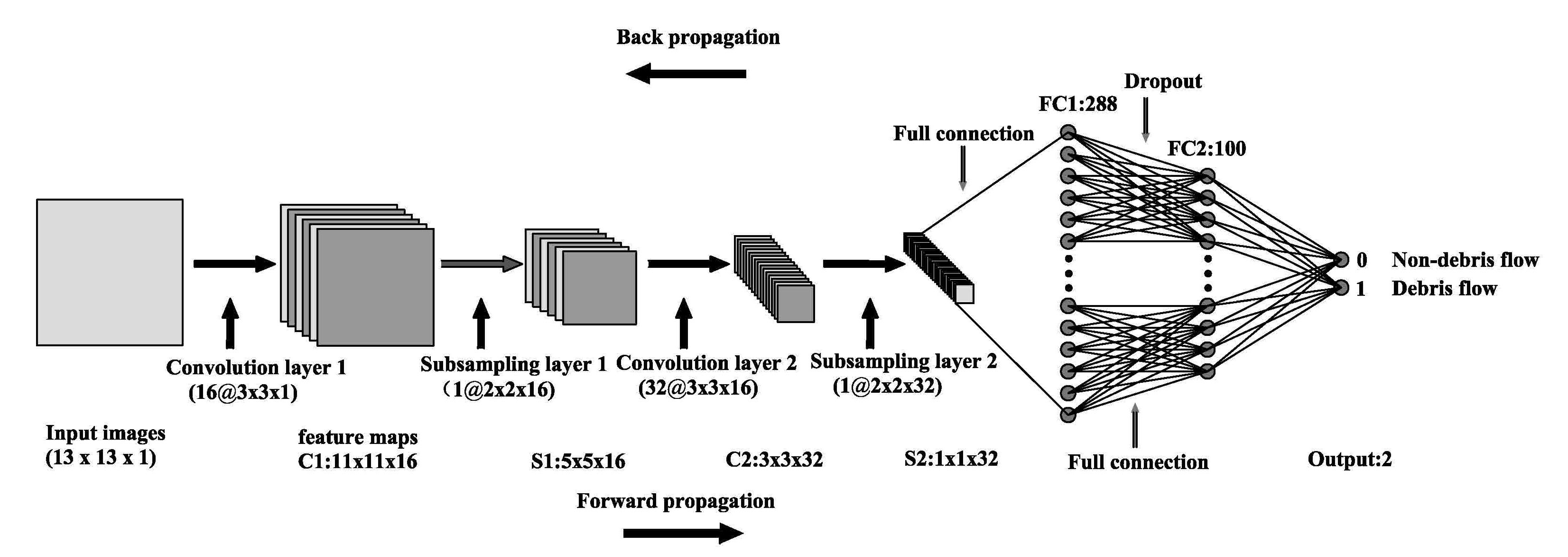
In the paper, the LetNet–5 structure was used which was the first proposed structure in the CNN algorithm [65]. The LetNet–5 structure (Figure 6) contains an input layer, two convolution layers, two subsampling layers, two full connection layers, and an output layer. The V–CNN based on the LetNet–5 structure was used in this research. Additionally, the backpropagation (BP) algorithm was utilized to modify the model parameters and increase model robustness. The V–CNN structure is shown in Figure 7.
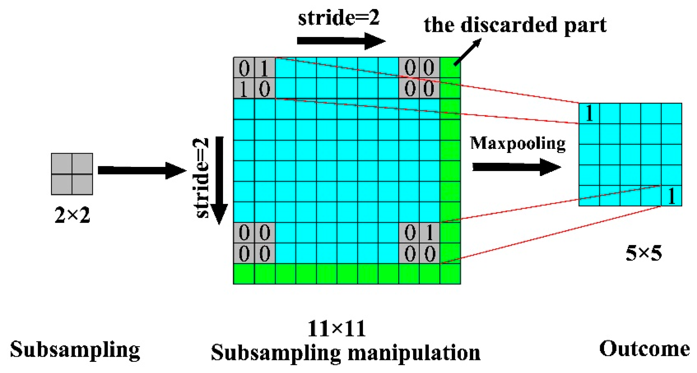
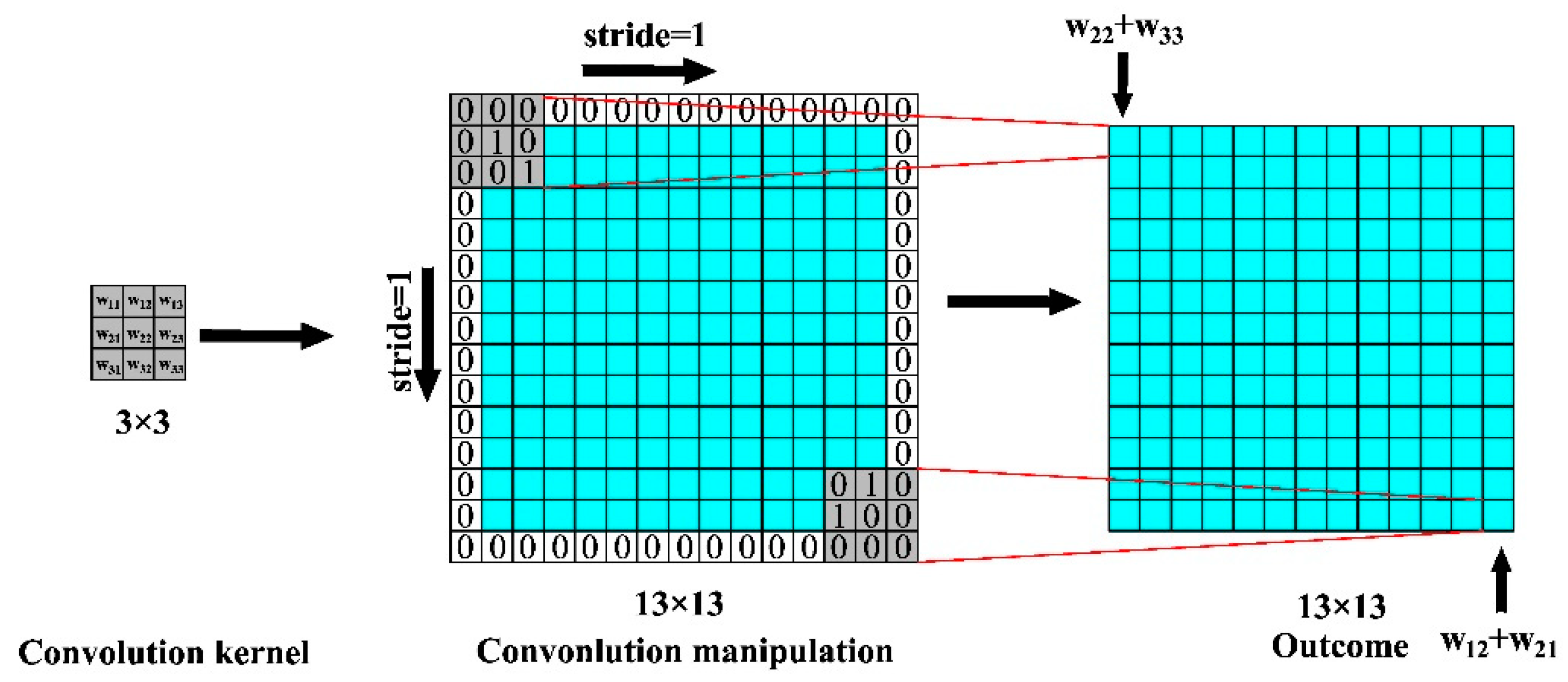
As we can see from the V–CNN structure, the input matrices become smaller after passing through the first convolution layer. VALID padding is used in this convolution manipulation, as shown in Figure 8. In this process, the sixteen convolution kernels with a size of 3 × 3 move across the matrices and perform the convolution calculation. Sixteen feature maps are obtained after the convolution manipulation and are fed into the first subsampling layer. Similarly, VALID padding is also used in the subsampling layer. The specific process used in the subsampling layer is shown in Figure 9. The max pooling manipulation takes the maximum value in a 2 × 2 region as the output. Because the subsampling kernels move two strides at a time, some data are directly discarded. After the matrices perform the first subsampling manipulation, sixteen feature maps with a size of 5 × 5 are produced.
Thirty–two convolution kernels with a size of 3 × 3 are utilized to perform the convolution manipulation. The matrices become smaller with a size of 3 × 3. After the second subsampling manipulation, the size of the matrices reduces to 1 × 1. Finally, the feature vectors are fed into the two full connection layers and the probability of debris flow occurring are determined by using the softmax classifier. To facilitate the adjustment of parameters and the establishment of the V–CNN model, a GUI based on python is used.
The V–CNN model is widely used for object recognition. During the convolution operation, the image edge information has limited use for object recognition. In other words, the image edge information is rarely used but the intermediate information is used many times, which results in an unbalanced use of information. During the subsampling operation, the V–CNN model discards the edge information, which has a limited impact on the main recognition process for the image. In this way, irrelevant data can be quickly discarded for the recognition of the photos to improve the recognition efficiency. It is important to note that if the size of the feature images is even, the subsampling operation will not discard the edge data but will still weaken the edge information of the image during the convolution operation. There is no doubt that the V–CNN model has the advantages of reduced computation time and rapid recognitions for objects. However, the purpose of this paper is not to identify objects but to search for the deep data relationships between debris flow data and the occurrence of debris flows. Therefore, it is not adequate to use VALID padding to process the data because debris flow data is too important to be discarded.

3.5. S–CNN

Compared to VALID padding, SAME padding approach is used for the first time in DFSM. The S–CNN model based on the SAME padding is proposed for use in this study, as shown in Figure 10.
As we can see from the S–CNN structure, after the input matrices pass through the first convolution layer, the matrix size does not change. The SAME padding approach is used in this convolution manipulation as shown in Figure 11. In the process of convolution manipulation, zeros are filled around the input matrices. For example, the input matrices are a size of p × p and the convolution kernel is a size of n × n. By using SAME padding, the matrices with a size of (p + n − 1) × (p + n − 1) are processed with convolution manipulation. Then, the feature maps with a size of p × p are created, which means that the size of the matrices before and after the convolution manipulation are the same. Next, the max pooling layer is used to perform the subsampling manipulation and zeros are filled around the feature maps as shown in Figure 12. It is obvious that no data were discarded by using SAME padding. After the second subsampling layer, the size of the matrices becomes 4 × 4 which means that more feature vectors are obtained. At last, by using two full connection layers and the softmax classifier, the probability distribution of two classified objects is obtained. Similarly, the GUI is used to adjust parameters and train the S–CNN model.
The S–CNN model is more suitable for the study of debris flows because this method uses the data in a balanced way and does not discard the edge information. During the convolution operation, to increase the efficiency of the use of matrices edge information and retain all data, the S–CNN model adds a certain range of blank areas around the matrices, but these areas have no impact on our calculation results. Therefore, the matrix size remains the same before and after each convolution operation, which means that all debris flow data are used equitably and kept intact. In the subsampling operation, to use the matrices edge information, a certain range of blank areas are also added to the matrices edge. These blank areas are still not involved in the calculation, thus increasing the use efficiency of debris flow data. No matter if the matrix size is odd or even, the data are not discarded during the subsampling operation. Debris flow data is very valuable, so the benefit of using SAME padding is to fully exploit the value of each piece of data. Therefore, the S–CNN model has great advantages compared with the V–CNN model in mining the relationship between debris flow data and debris flows occurring.

3.6. Model Evaluation

Without model evaluations, this research would be meaningless [66]. As far as we know, the ROC curve is normally used to evaluate the models in classification problems. The ROC curve distinguishes the two categories by a diagnostic test based on the distribution of correct and incorrect predictions according to a 2 × 2 contingency table (Table 3) [67]. The ROC curve takes 1–Specificity (FP rate) and Sensitivity (TP rate) as the abscissa and ordinate, respectively. In this paper, the TP rate represents the proportion of disaster locations that are correctly classified as debris flows, and the FP rate represents the proportion of non–disaster locations that are wrongly classified as debris flows. Additionally, the area under the ROC curve (AUC) is an important index to measure the predictive capability of a model. In general, the closer the AUC value is to 1, the better the model.
Some mathematical–statistical methods were also utilized to measure the predictive ability of the models, such as ACC, F–measure, and MAE. The formulas for these evaluation indicators are as follows [68]:
S e n s i t i v i t y = T P T P + F N
S p e c i f i c i t y = T N F P + T N
A C C = T P + T N T N + F N + T P + F P
F m e a s u r e = 2 × S e n s i t i v i t y × S p e c i f i c i t y / ( S e n s i t i v i t y + S p e c i f i c i t y )
M A E = | p 1 t 1 | + | p 2 t 2 | + + | p n t n | n
where TP and TN represent the proportion which were correctly classified, while FP and FN represent the proportion which were incorrectly classified and p i and t i are the predicted and true values, respectively.

4. Results and Analysis

4.1. Multicollinearity Analysis Results

The tolerance and VIF values calculated by thirteen factors are shown in Table 4. In general, a VIF value greater than 10 or a tolerance value less than 0.1 indicates that the factor had strong collinearity, and should be discarded. The results show that vegetation coverage had a minimum tolerance value of 0.476, and a maximum VIF value of 2.099. Therefore, all thirteen influencing factors meet the collinearity requirements.

4.2. The Results of FR Method

The FR values are used to represent the correlation between debris flows and influencing factors. The calculation results are shown in Table 5. In general, the results indicate that the corresponding area is more prone to debris flow occurring when the FR value is greater than 1 [69].
The results demonstrated that elevation lower than 600 m had the highest probability of debris flow occurring in Jilin Province, China. In terms of the slope, the trend of the FR values was convex. Slopes from 5° to 10° had the highest FR value (1.923). Similarly, the trend of FR values for the aspect was convex. In addition, the southeast–facing aspect had the highest FR value of 1.524. Plan curvature of the concave class (1.208) and profile curvature of between 0.06 and 0.28 class (2.634) had higher FR values than the other classes. Meanwhile, TWI had the highest FR value of 2.199 between 9 and 11 and the lowest value of 0.677 between 5 and 7.
Additionally, the results also showed that distance to roads of less than 1000 m (1.353) was prone to debris flow, which had the highest FR value compared to other classes. On the other hand, distance to rivers of between 2000 m and 2500 m (1.975) and greater than 2500 m (0.950) had the highest and lowest probability of debris flow occurring, respectively. From the lithology point of view, group 3 has the highest FR value (5.462). The results also revealed that population density and annual rainfall values ranging from 10–100/km2 (1.239) and 600–800 mm (2.314), respectively, had a higher probability of debris flow occurring. For the topography factor, the valley areas obtained the highest FR value (2.370). Compared to the four classes of vegetation coverage, we found that the moderate class (1.933) and the low class (0.172) had the highest and lowest FR values.

4.3. The Results of GR Method

The results are shown in Figure 13. The selection of influencing factors can be supported by the GR method. Factors with higher AM values are more significant to the models, whereas factors with AM values of 0 cannot contribute to debris flow susceptibility modeling and should be excluded. It was obvious that lithology had the highest AM values of 0.085, followed by distance to roads (0.083), rainfall (0.077), topography (0.065), population density (0.062), elevation (0.059), profile curvature (0.057), TWI (0.053), plan curvature (0.047), aspect (0.046), vegetation coverage (0.036), distance to rivers (0.024), and slope (0.018). Therefore, all influencing factors have sufficient predictive ability to complete the establishment of models.

4.4. Production of the Debris Flow Susceptibility Maps

In the paper, grid cells with a size of 100 m × 100 m were utilized to make the debris flow susceptibility maps. We used the LetNet–5 structure to build the S–CNN and V–CNN models by using the same training set. All codes are implemented using Python under the TensorFlow framework. TensorFlow is a Google open–source software that is widely used in DL algorithms [70,71]. The main compiler was PyCharm5.0.3, which was used for building the S–CNN and V–CNN models and doing the GUI production. The adjustment of hyperparameters was mainly carried out by using the GUI, and the final parameters were determined through a trial–and–error method and previous experts’ previous experience, as shown in Table 6.
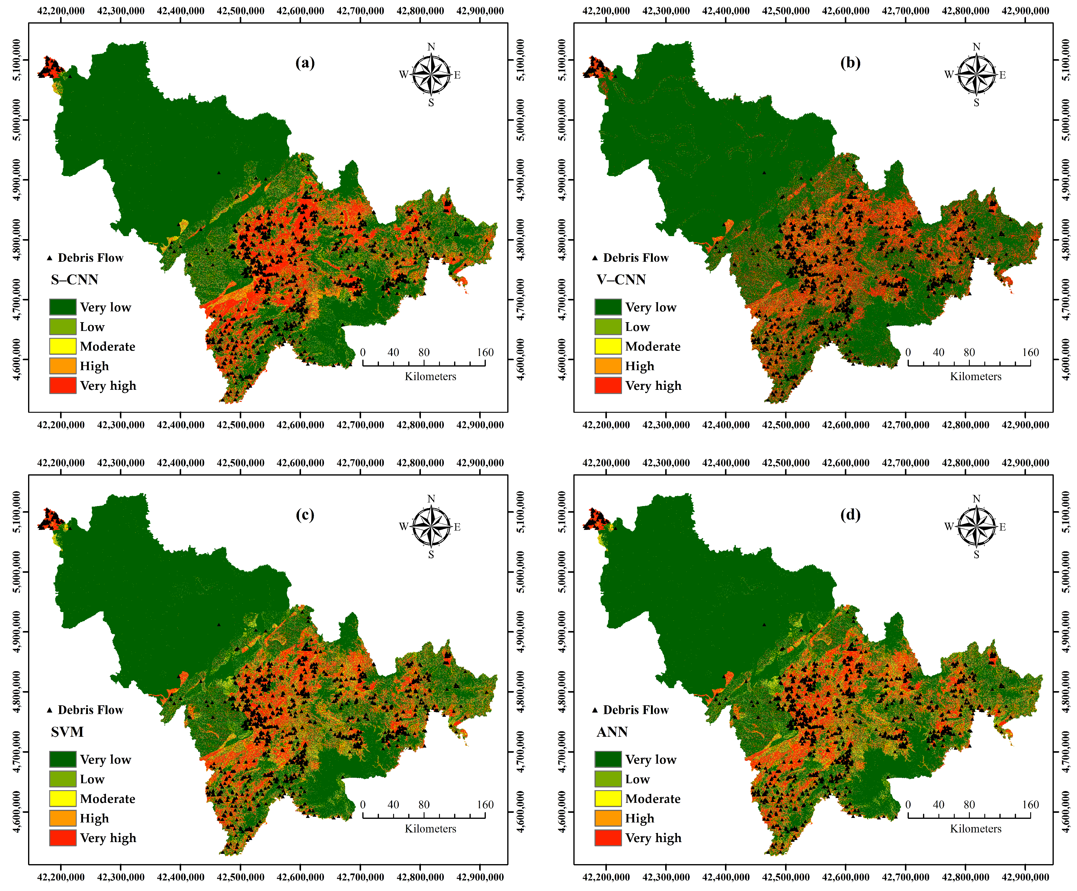
Next, we used the training set to train the S–CNN model, and the model applied to the whole research area after the validation set reached a certain accuracy. The probability of debris flow in each grid cell was obtained. The debris flow susceptibility map was generated in an arcgis10.5 environment by using the point to raster tool. For better visualization, the debris flow susceptibility map was divided into five classes of very low, low, moderate, high, and very high by natural breaks method, as shown in Figure 14a. The area percentages of each class were 69.92% (very low), 4.11% (low), 3.92% (moderate), 5.32% (high), and 16.73% (very high). To facilitate the comparison of susceptibility maps, the same break values of the classes as the S–CNN model were used for all the maps.
The V–CNN model was applied to the study area similarly. Then the debris flow susceptibility map using the V–CNN model was produced, as shown in Figure 14b. And the area percentages of each class were 73.36% (very low), 2.15% (low), 2.01% (moderate), 3.66% (high), and 18.82% (very high).
In the SVM model, the radial basis function (RBF) kernel was applied [72,73,74]. The penalty coefficient C and kernel width γ were used after the trial–and–error method. In the optimization function, the penalty coefficient C mainly balanced the relationship between the complexity of the model and the misclassification rate, which can be understood as the regularization coefficient and kernel width γ mainly defined the influence of a single sample on the entire classification hyperplane [73]. Finally, the optimized C and γ were determined to be 1, and 0.1, respectively. The model building process and the production of debris–flow susceptibility maps were mainly implemented in an IBM SPSS Modeler18.0 and arcgis10.5 environment. Similarly, the debris flow susceptibility map was also reclassified into five classes of very low, low, moderate, high, and very high, as shown in Figure 14c. The results showed that the very low class had the largest percentage of 68.42%, followed by very high (14.46%), low (6.55%), high (5.65%), and moderate (4.92%).
In this paper, the multilayer perceptron with two hidden layers was used to build the ANN model [75,76,77]. To ascertain whether the convolutional layers and subsampling layers can mine more information from the data, the two hidden layers used the same number of neurons as the full connection layers. Meanwhile, the logistic sigmoid was utilized to determine the probability of a debris flow occurring. Then the ANN model was constructed using the training set in an IBM SPSS Modeler18.0 environment. Similarly, the debris flow susceptibility map was produced in an arcgis10.5 environment. In the same way, the debris flow susceptibility map was reclassified into five classes as very low, low, moderate, high, and very high, as shown in Figure 14d. The results showed that the very low class had the largest percentage of 72.35%, followed by very high (12.64%), high (9.26%), moderate (3.12%), and low (2.63%).

4.5. Model Validation

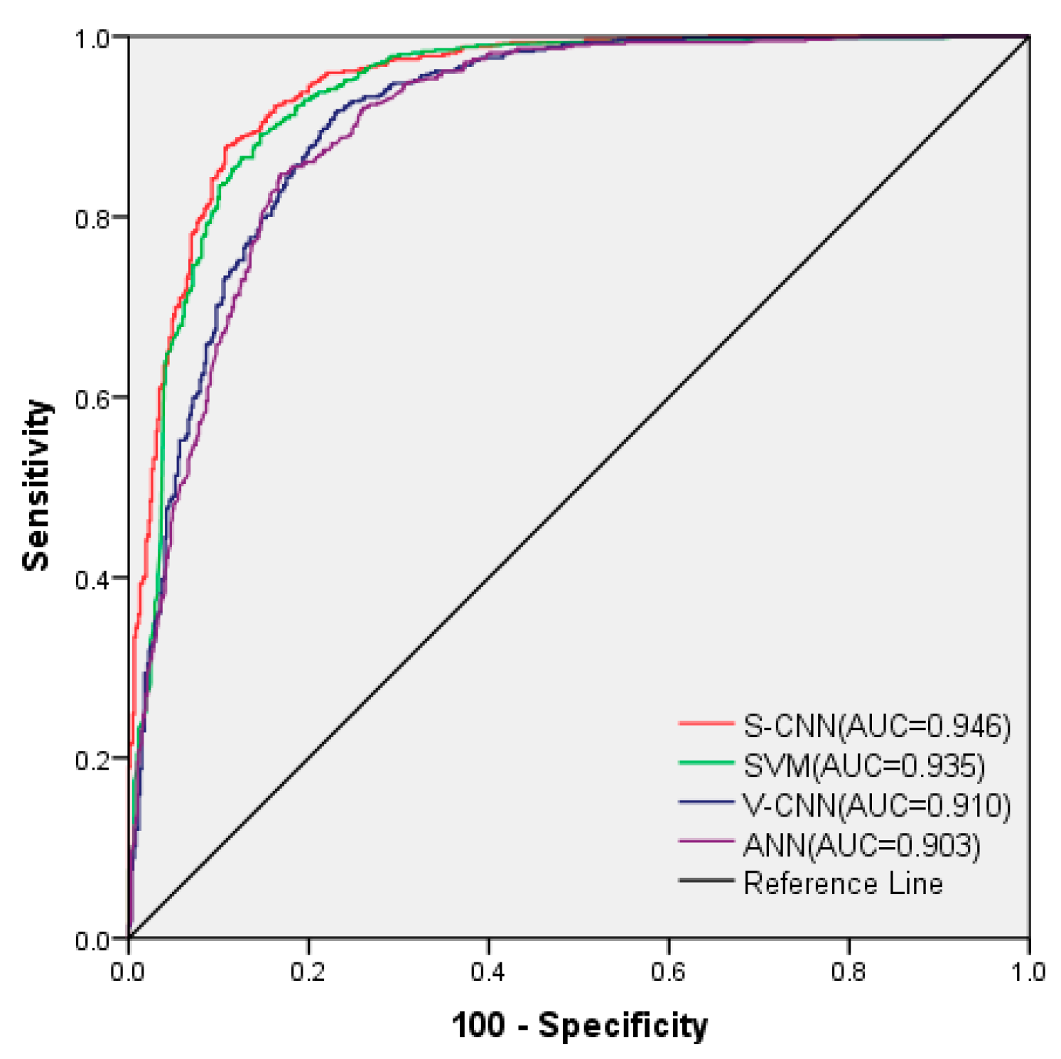
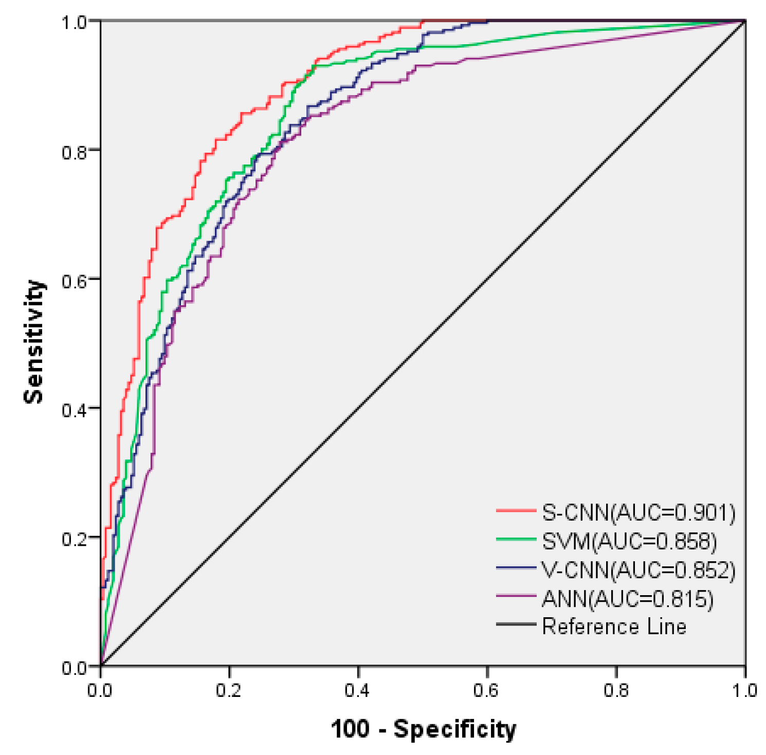
The results of the ROC curves and AUC values of the four models using the training set and validation set are shown in Figure 15 and Figure 16. It was obvious that the S–CNN model had the highest AUC value of 0.946 in the training set, followed by the SVM model (0.935), the V–CNN model (0.910), and the ANN model (0.903). In addition, the validation set showed that the S–CNN model had the highest AUC value of 0.901, followed by the SVM model (0.858), the V–CNN model (0.852) and the ANN model (0.815) which meant that the S–CNN model had the best predictive ability over the other three models.
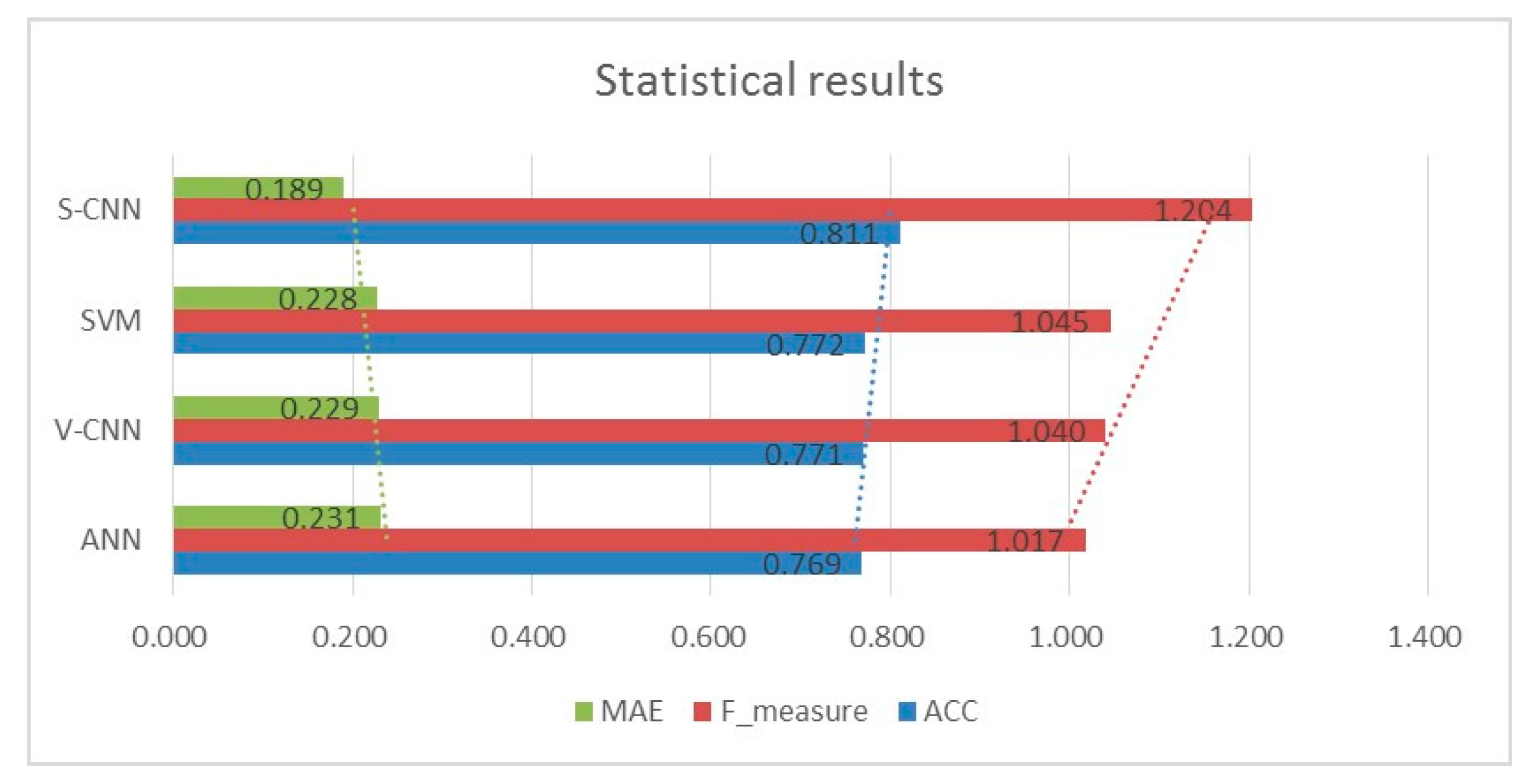
Additionally, three other statistical methods, ACC, F–measure, and MAE, were also used to compare the model’s accuracy using the validation set. The results were shown in Figure 17. It was obvious that the S–CNN model had the highest ACC value (0.811), the highest F–measure value (1.204), and the lowest MAE value (0.189), which meant that the S–CNN model was better than the other three models. The comparison results of the statistical methods and ROC curves were consistent, which proved that the S–CNN model can effectively improve the spatial prediction accuracy of DFSM.
Figure 18 shows the percentage of the five classes of the different models in DFSM. The results of the four models were acceptable according to the hierarchical distribution. In the very low grade, the V–CNN model had the highest proportion of 73.36% and the SVM model had the lowest proportion of 68.42%, which indicated that most of the research area was in the very low grade. In the low grade, the highest value was 6.55% in the SVM model and the lowest value was 2.15% in the V–CNN model. In the moderate grade, the proportion of the four models was significantly different, including the SVM model (4.92%), the S–CNN model (3.92%), the ANN model (3.12%) and the V–CNN model (2.01%). In the high grade, the ANN model had the highest value of 9.26% and the V–CNN model had the lowest value of 3.66%. For the very high grade, the V–CNN model had the highest value of 18.82%, followed by the S–CNN model (16.73%), the SVM model (14.46%), and the ANN model (12.64%). To more accurately compare susceptibility maps, a comparison of the susceptibility values was carried out on a pixel–by–pixel basis, to reveal spatial patterns in the differences among susceptibility maps [78]. And the results were shown in Figure 19. The model with a higher AUC value was selected as the benchmark, and six comparison maps were obtained, namely “S–CNN and SVM”, “S–CNN and V–CNN”, “S–CNN and ANN”, “SVM and V–CNN”, ”SVM and ANN”, and “V–CNN and ANN”. It was obvious that the relevant differences were encountered and not evenly distributed. Some spatial features can be observed in almost every comparison map. The difference was mainly in the southeast of Jilin Province, where 94% debris flows occurred. It can be inferred that the greater the difference of AUC values between models, the more obvious the relevant difference in the comparison maps.

5. Discussion

DFSM is one of the most effective approaches for debris flow evaluation and management tasks. Although many methods have been applied to DFSM, there is no benchmark for model selection. In this paper, four models (S–CNN, V–CNN, SVM, ANN) were used to study the spatial distribution of debris–flow susceptibility in Jilin Province, China.
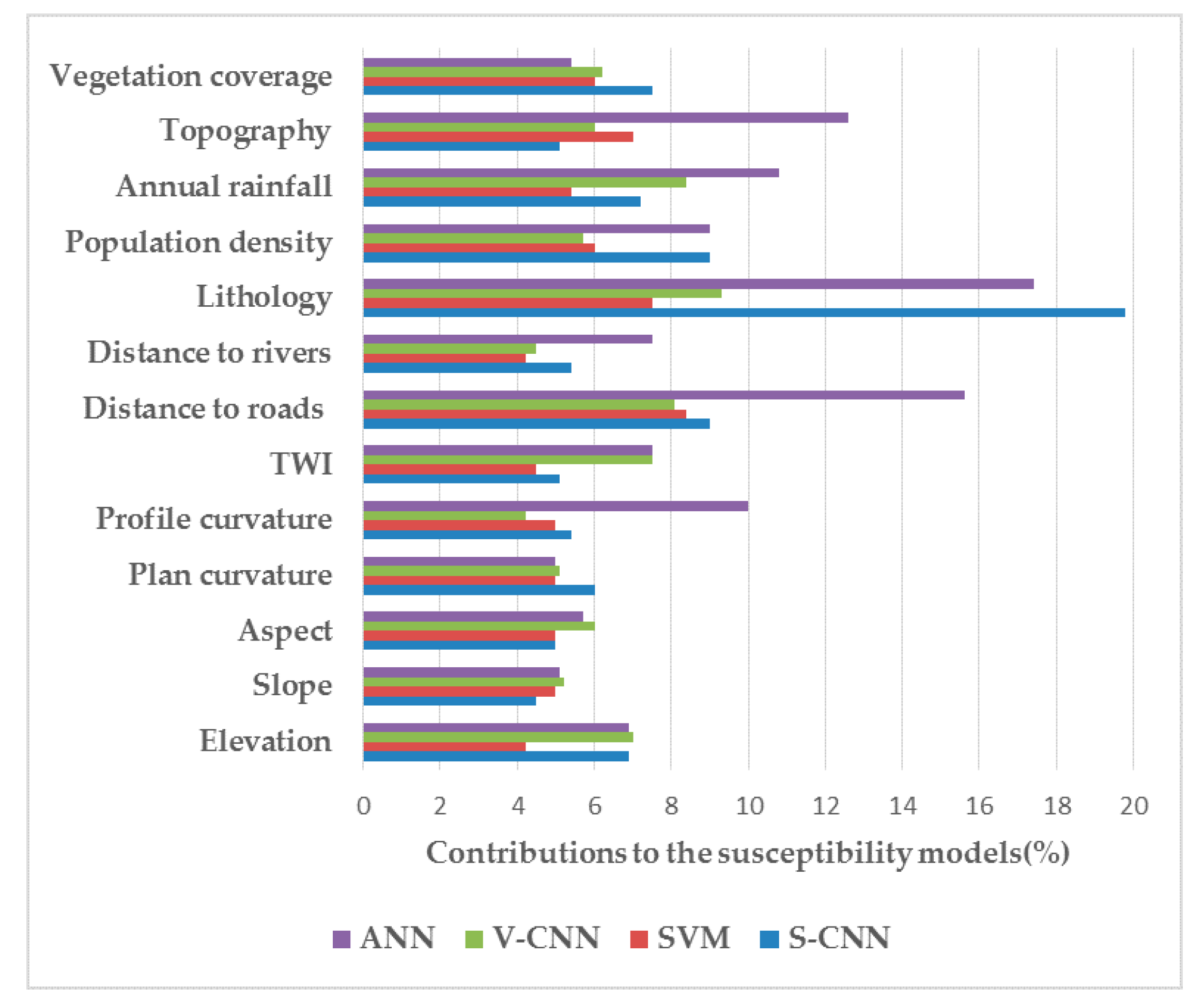
To ensure the quality of the models, influencing factors selection is essential. Then a multicollinearity test was prepared. The results showed that all influencing factors were independent and effective (Table 4). The results of the GR method (Figure 13) showed that all influencing factors had enough predictive ability for the occurrence of debris flows. In addition, the FR method was introduced to measure the relationships between influencing factors and debris flows (Table 5). The results showed that debris flows had the greatest impact on low elevation terrain. The reason may be that the area with low elevation has a larger slope value in the research area. Slopes from 5° to 10° had the highest FR value (1.923). The main reason may be that there are less vegetation coverage and sufficient rain in this area. The southeast aspect had the highest effect on debris flows because the southeast aspect may have the most wetness among other aspects. Regarding the plan curvature, the concave had the highest effect on debris flows occurring. This result may be closely related to human engineering activities. The relationships between profile curvature and debris flows were roughly linear. The profile curvature between 0.06 and 0.28 had the highest impact on debris flow occurrences which had the biggest catchment area. TWI represents the ability of soil moisture to reach saturation. In this research, TWI values between 9 and 11 had the highest impact on debris flows. The distances less than 1000 m from the road exerted the highest impact on debris flow occurring since the closer to the road, the stronger the human activity. The distances between 2000 to 2500 m from the river had the highest FR value (1.975). This may be related to the density of the river networks. Although most debris flows are distributed in group 1 and group 2 area, group 3 had the highest relationship on debris flow occurrences. This may be closely related to the terrain conditions and the anti–weathering ability of rocks in the southeast of Jilin Province. Population density between 10 and 100/km2 had the highest FR value. It can be inferred from the topography factor that the class (10–100/km2) is located in mountainous areas, so it is closely related to the occurrence of debris flows. From the perspective of annual rainfall, the 600–800 mm class was most closely associated with debris flows. This may be related to the dual effect of rainfall and soil. In addition, the valley area was most closely related to debris flows among the four topography class. This is mainly due to the dense distribution of rivers and the large slope of the slope in the area. It can be seen from vegetation cover that debris flows mostly occurred in areas with more vegetation because the areas are mostly mountainous and receive plenty of rain. To find out the contribution of influencing factors to the distribution of debris–flow susceptibility, we excluded one factor in turn to construct the four models. The results were shown in Figure 20. All influencing factors have contributed to the distribution of debris–flow susceptibility. Lithology has the highest contribution value of 19.8% in the S–CNN model, while elevation and distance to rivers have the lowest contribution value of 4.2% in the SVM model. The same factor has different contributions on different models. The difference between the SVM and V–CNN models is small, but the difference between the S–CNN and ANN models is large.
The ROC curve results showed that the accuracy of the S–CNN model was far higher than that of the other three models, which indicated that the CNN structure that used SAME padding had the highest accuracy in a debris flow susceptibility evaluation. Then some detailed comparisons can be summarized as follows. First, for the V–CNN and ANN models, the accuracy of the V–CNN model was 0.852 in the validation set, which was higher than that of the ANN model (0.815) when they were inputted with the same data, indicating that the convolution layers and subsampling layers uncovered more effective information from the data that made the model more accurate. This comparative case showed that the CNN model was indeed available and better than the ANN model for debris flow susceptibility assessments. Second, by comparing the SVM and V–CNN models, we found that the accuracy of the SVM model was 0.6% higher than that of the V–CNN model in the validation set. The reason was that the convolution layers and subsampling layers used VALID padding to process the data, resulting in the loss of debris flow information (See Figure 8 and Figure 9), which made the accuracy of the V–CNN model lower than that of the SVM model.
Therefore, we used a different method named SAME padding to process the data. On this basis, the S–CNN model can make full use of all the information in the process of convolution and subsampling operations compared with the V–CNN model (See Figure 11 and Figure 12). As we can see, the matrices became smaller after the convolution operation by the use of VALID padding. It meant that the edge information of the matrices was used only once but the information in the middle of the images was used many times, which led to the unbalanced use of the information. In contrast, SAME padding added a certain range of blank areas around the matrices during the convolution manipulation, which meant that all the data were used evenly. During the max pooling manipulation, VALID padding discarded the edge information of the matrices, which resulted in the loss of debris flow data. However, SAME padding also added a certain range of blank areas around the matrices, and then all the information can be used effectively. Therefore, the S–CNN model can definitely obtain a more accurate debris flow susceptibility map compared with the V–CNN model. Finally, it was found that the accuracy of the S–CNN model was 4.3% higher than that of the SVM model in the validation set, which meant that SAME padding was more suitable to handle the debris flow data than VALID padding because SAME padding in the CNN structure can make full use of the debris flow data and extract more valuable information than the V–CNN model.
The differences between CNN and traditional ML algorithms (SVM and ANN) can be summarized as follows. First, the format of input data is different. The input data of CNN and traditional ML algorithms are 4D–tensor and text format, respectively. Second, the structures of the algorithms are different. The convolution and subsampling layers are unique structures in CNN. The function of convolution layers is to extract different features of input data. The subsampling layers are used to compress the extracted features. Third, the means of building models are different. CNN and traditional ML algorithms are based on TensorFlow framework and SPSS Modeler software to build models, respectively.
The strength of this paper is the successful application of 2D–CNN to a susceptibility evaluation of debris flow and the use of the S–CNN model for the first time to study the debris flow susceptibility in Jilin Province. Compared with the traditional ML methods, the S–CNN model used the convolution and subsampling operations to dig out more rules from the data. In contrast to the V–CNN model, the S–CNN model can retain data and use it completely. The ROC curves and three statistical methods results show that the S–CNN model had the best performance. And the shortcomings of this paper are the uncertainty of the CNN model parameters and structure. At present, there is no accepted standard for selecting CNN parameters and structures. Both the parameters and the structure are the local optimal solutions acquired after continuous attempts. This paper used the LetNet–5 structure, and the size of the convolution and subsampling layers were derived from experience, which made the precision of the CNN model was not necessarily optimal. This also points out a potential new direction for our research, namely, the optimization of CNN parameters.

6. Conclusions

In debris flow prone areas, it is very important to establish a robust, stable and accurate model for the spatial prediction of debris flow susceptibility. Although many well–performing models have been used in regional research, there is still room for improvement in increasing model accuracy. For this reason, we have carried out the research in this paper. Then the following conclusions can be inferred.
  • The AUC value of the V–CNN model (0.852) was higher than that of the ANN model (0.815). And three mathematical statistical methods also showed that the V–CNN model had smaller errors. The research indicated that the convolution layers and max pooling layers can extract more data patterns than pure full connection layers. Therefore, CNN models are more suitable for studying debris flow susceptibility than traditional ML methods such as ANN.
  • The CNN models based on VALID padding still have some shortcomings. From the ROC caves and mathematical statistics, the accuracy of the V–CNN model was lower than that of the SVM model. This indicated that the method of VALID padding processing of the data was not the optimal choice. Therefore, SAME padding was selected to process debris flow data in this paper.
  • SAME padding is more suitable for processing debris flow data compared with VALID padding. The S–CNN model obtained the highest AUC value and the minimum error. Obviously, the S–CNN model can make full use of the data and dig out more valuable information than the other three models.
  • We compare the susceptibility maps on a pixel–by–pixel basis and six comparison maps are produced. By observing the differences distribution of comparison maps, we draw a conclusion that the highest AUC map may not have the best predictive ability in some areas. This may be related to geotechnical and geomorphological reasons of differences and systematic errors.

Author Contributions

Conceptualization, S.Q.(Shengwu Qin) and Y.C.; methodology, Y.C.; software, Y.C.; validation, W.C., Y.C., G.S., and J.Y.; formal analysis, Y.C.; data curation, Q.D. and Y.C.; writing—original draft preparation, Y.C., U.E.N.; writing—review and editing, Y.C., S.Q.(Shuangshuang Qiao), and J.Y.; visualization, Y.C.; supervision, S.Q.(Shengwu Qin); project administration, S.Q.(Shengwu Qin); funding acquisition, S.Q.(Shengwu Qin). All authors have read and agreed to the published version of the manuscript.

Funding

This research was funded by the Jilin Provincial Science and Technology Department (No.20190303103SF). National Natural Science Foundation of China (Grant no 41977221).

Conflicts of Interest

The authors declare no conflict of interest.

References

  1. Dowling, C.A.; Santi, P.M. Debris flows and their toll on human life: A global analysis of debris–flow fatalities from 1950 to 2011. Nat. Hazards 2014, 71, 203–227. [Google Scholar] [CrossRef]
  2. Xu, Q.; Zhang, S.; Li, W.L.; van Asch, T.W.J. The 13 August 2010 catastrophic debris flows after the 2008 Wenchuan earthquake, China. Nat. Hazards Earth Syst. Sci. 2012, 12, 201–216. [Google Scholar] [CrossRef]
  3. Iverson, R.M. Debris flows: Behavior and hazard assessment. Geol. Today 2014, 30, 15–20. [Google Scholar] [CrossRef]
  4. Zhou, G.G.D.; Cui, R.; Tang, J.B.; Chen, H.Y.; Zou, Q.; Sun, Q.C. Experimental study on the triggering mechanisms and kinematic properties of large debris flows in Wenjia Gully. Eng. Geol. 2015, 194, 52–61. [Google Scholar] [CrossRef]
  5. Westen, C.J.V.; Asch, T.W.J.V.; Soeters, R. Landslide hazard and risk zonation—why is it still so difficult? Bull. Eng. Geol. Environ. 2006, 65, 167–184. [Google Scholar] [CrossRef]
  6. Brabb, E.E. Innovative approaches to landslide hazard mapping. In Proceedings of the Fourth International Symposium on Landslides, Canadian Geotechnical Society, Toronto, SD, Canada, 16–21 September 1984; pp. 307–324. [Google Scholar]
  7. Reichenbach, P.; Rossi, M.; Malamud, B.D.; Mihir, M.; Guzzetti, F. A review of statistically–based landslide susceptibility models. Earth-Sci. Rev. 2018, 180, 60–91. [Google Scholar] [CrossRef]
  8. Pourghasemi, H.R.; Yansari, Z.T.; Panagos, P.; Pradhan, B. Analysis and evaluation of landslide susceptibility: A review on articles published during 2005–2016 (periods of 2005–2012 and 2013–2016). Arab. J. Geosci. 2018, 11, 193. [Google Scholar] [CrossRef]
  9. Wu, Y.; Li, W.; Liu, P.; Bai, H.; Wang, Q.; He, J.; Liu, Y.; Sun, S. Application of analytic hierarchy process model for landslide susceptibility mapping in the Gangu County, Gansu Province, China. Environ. Earth Sci. 2016, 75, 422. [Google Scholar] [CrossRef]
  10. Quan, H.; Lee, B. GIS–based landslide susceptibility mapping using analytic hierarchy process and artificial neural network in Jeju (Korea). KSCE J. Civ. Eng. 2012, 16, 1258–1266. [Google Scholar] [CrossRef]
  11. Quan, H.; Moon, H.D.; Jin, G. Landslide Susceptibility Analysis in Baekdu Mountain Area Using ANN and AHP Method. J. Korean Geoenviron. Soc. 2014, 15, 79–85. [Google Scholar] [CrossRef] [Green Version]
  12. Dhianaufal, D.; Kristyanto, T.H.W.; Indra, T.L.; Syahputra, R. Fuzzy Logic Method for Landslide Susceptibility Mapping in Volcanic Sediment Area in Western Bogor. AIP Conf. Proc. 2018, 2023, 020190. [Google Scholar] [CrossRef]
  13. Basofi, A.; Fariza, A.; Dzulkarnain, M.R. Landslides Susceptibility Mapping Using Fuzzy Logic: A Case Study in Ponorogo. In Proceedings of the 2016 International Conference on Data and Software Engineering (ICoDSE), East Java, Indonesia, 26–27 October 2016. [Google Scholar]
  14. Pradhan, B. Use of GIS–based fuzzy logic relations and its cross application to produce landslide susceptibility maps in three test areas in Malaysia. Environ. Earth Sci. 2011, 63, 329–349. [Google Scholar] [CrossRef]
  15. Hong, H.; Ilia, I.; Tsangaratos, P.; Chen, W.; Xu, C. A hybrid fuzzy weight of evidence method in landslide susceptibility analysis on the Wuyuan area, China. Geomorphology 2017, 290, 1–16. [Google Scholar] [CrossRef]
  16. Regmi, A.D.; Yoshida, K.; Pourghasemi, H.R.; Dhital, M.R.; Pradhan, B. Landslide susceptibility mapping along Bhalubang—Shiwapur area of mid–Western Nepal using frequency ratio and conditional probability models. J. Mt. Sci. 2014, 11, 1266–1285. [Google Scholar] [CrossRef]
  17. Razavizadeh, S.; Solaimani, K.; Massironi, M.; Kavian, A. Mapping landslide susceptibility with frequency ratio, statistical index, and weights of evidence models: A case study in northern Iran. Environ. Earth Sci. 2017, 76, 499. [Google Scholar] [CrossRef]
  18. Huang, F.; Cao, Z.; Guo, J.; Jiang, S.; Li, S.; Guo, Z. Comparisons of heuristic, general statistical and machine learning models for landslide susceptibility prediction and mapping. Catena 2020, 191, 104580. [Google Scholar] [CrossRef]
  19. Aditian, A.; Kubota, T.; Shinohara, Y. Comparison of GIS–based landslide susceptibility models using frequency ratio, logistic regression, and artificial neural network in a tertiary region of Ambon, Indonesia. Geomorphology 2018, 318, 101–111. [Google Scholar] [CrossRef]
  20. Kavzoglu, T.; Sahin, E.K.; Colkesen, I. Landslide susceptibility mapping using GIS–based multi–criteria decision analysis, support vector machines, and logistic regression. Landslides 2014, 11, 425–439. [Google Scholar] [CrossRef]
  21. Kumar, D.; Thakur, M.; Dubey, C.S.; Shukla, D.P. Landslide susceptibility mapping & prediction using Support Vector Machine for Mandakini River Basin, Garhwal Himalaya, India. Geomorphology 2017, 295, 115–125. [Google Scholar]
  22. Kalantar, B.; Pradhan, B.; Naghibi, S.A.; Motevalli, A.; Mansor, S. Assessment of the effects of training data selection on the landslide susceptibility mapping: A comparison between support vector machine (SVM), logistic regression (LR) and artificial neural networks (ANN). Geomat. Nat. Hazards Risk 2018, 9, 49–69. [Google Scholar] [CrossRef]
  23. Tsangaratos, P.; Ilia, I. Comparison of a logistic regression and Naive Bayes classifier in landslide susceptibility assessments: The influence of models complexity and training dataset size. Catena 2016, 145, 164–179. [Google Scholar] [CrossRef]
  24. Gelisli, K.; Kaya, T.; Babacan, A.E. Assessing the factor of safety using an artificial neural network: Case studies on landslides in Giresun, Turkey. Environ. Earth Sci. 2015, 73, 8639–8646. [Google Scholar] [CrossRef]
  25. Dieu, T.B.; Tran, A.T.; Klempe, H.; Pradhan, B.; Revhaug, I. Spatial prediction models for shallow landslide hazards: A comparative assessment of the efficacy of support vector machines, artificial neural networks, kernel logistic regression, and logistic model tree. Landslides 2016, 13, 361–378. [Google Scholar]
  26. Pourghasemi, H.R.; Kerle, N. Random forests and evidential belief function–based landslide susceptibility assessment in Western Mazandaran Province, Iran. Environ. Earth Sci. 2016, 75. [Google Scholar] [CrossRef]
  27. Kim, J.; Lee, S.; Jung, H.; Lee, S. Landslide susceptibility mapping using random forest and boosted tree models in Pyeong–Chang, Korea. Geocarto Int. 2018, 33, 1000–1015. [Google Scholar] [CrossRef]
  28. Xiong, K.; Adhikari, B.R.; Stamatopoulos, C.A.; Zhan, Y.; Wu, S.; Dong, Z.; Di, B. Comparison of Different Machine Learning Methods for Debris Flow Susceptibility Mapping: A Case Study in the Sichuan Province, China. Remote Sens. 2020, 12, 295. [Google Scholar] [CrossRef] [Green Version]
  29. Esper Angillieri, M.Y. Debris flow susceptibility mapping in a portion of the Andes and Preandes of San Juan, Argentina using frequency ratio and logistic regression models. Earth Sci. Res. J. 2013, 17, 159–167. [Google Scholar]
  30. Wang, Y.; Fang, Z.C.; Hong, H.Y. Comparison of convolutional neural networks for landslide susceptibility mapping in Yanshan County, China. Sci. Total Environ. 2019, 666, 975–993. [Google Scholar] [CrossRef]
  31. Ma, Z.; Qin, S.; Cao, C.; Lv, J.; Li, G.; Qiao, S.; Hu, X. The Influence of Different Knowledge–Driven Methods on Landslide Susceptibility Mapping: A Case Study in the Changbai Mountain Area, Northeast China. Entropy 2019, 21, 372. [Google Scholar] [CrossRef] [Green Version]
  32. Qiao, S.; Qin, S.; Chen, J.; Hu, X.; Ma, Z. The Application of a Three-Dimensional Deterministic Model in the Study of Debris Flow Prediction Based on the Rainfall–Unstable Soil Coupling Mechanism. Processes 2019, 7, 99. [Google Scholar] [CrossRef] [Green Version]
  33. Ghorbanzadeh, O.; Blaschke, T.; Gholamnia, K.; Meena, S.R.; Tiede, D.; Aryal, J. Evaluation of Different Machine Learning Methods and Deep–Learning Convolutional Neural Networks for Landslide Detection. Remote Sens. 2019, 11, 196. [Google Scholar] [CrossRef] [Green Version]
  34. Vu, D.P.; Quoc–Huy, N.; Huu–Duy, N.; Van–Manh, P.; Van Manh, V.; Quang–Thanh, B. Convolutional Neural Network & x2014; Optimized Moth Flame Algorithm for Shallow Landslide Susceptible Analysis. IEEE Access 2020, 8, 32727–32736. [Google Scholar]
  35. Ullo, S.L.; Langenkamp, M.S.; Oikarinen, T.P.; Del Rosso, M.P.; Sebastianelli, A.; Piccirillo, F.; Sica, S. Landslide Geohazard Assessment With Convolutional Neural Networks Using Sentinel–2 Imagery Data. In Proceedings of the IEEE International Symposium on Geoscience and Remote Sensing IGARSS, Yokohama, Japan, 28 July–2 August 2019. [Google Scholar] [CrossRef] [Green Version]
  36. Cheng, G.; Ma, C.; Zhou, P.; Yao, X.; Han, J. Scene classification of high resolution remote sensing images using convolutional neural networks. In Proceedings of the 2016 IEEE International Geoscience and Remote Sensing Symposium (IGARSS), Beijing, China, 10–15 July 2016. [Google Scholar]
  37. Krizhevsky, A.; Sutskever, I.; Hinton, G. ImageNet Classification with Deep Convolutional Neural Networks. Adv. Neural Inf. Process. Syst. 2012, 25, 6. [Google Scholar] [CrossRef]
  38. Galli, M.; Ardizzone, F.; Cardinali, M.; Guzzetti, F.; Reichenbach, P. Comparing landslide inventory maps. Geomorphology 2008, 94, 268–289. [Google Scholar] [CrossRef]
  39. Guzzetti, F.; Mondini, A.C.; Cardinali, M.; Fiorucci, F.; Santangelo, M.; Chang, K. Landslide inventory maps: New tools for an old problem. Earth-Sci. Rev. 2012, 112, 42–66. [Google Scholar] [CrossRef] [Green Version]
  40. Dou, Q.; Qin, S.W.; Zhang, Y.C.; MA, Z.J.; Chen, J.; Qiao, S.; Hu, X.; Liu, F. A Method for Improving Controlling Factors Based on Information Fusion for Debris Flow Susceptibility Mapping: A Case Study in Jilin Province, China. Entropy 2019, 21, 695. [Google Scholar] [CrossRef] [Green Version]
  41. Conforti, M.; Pascale, S.; Robustelli, G.; Sdao, F. Evaluation of prediction capability of the artificial neural networks for mapping landslide susceptibility in the Turbolo River catchment (northern Calabria, Italy). Catena 2014, 113, 236–250. [Google Scholar] [CrossRef]
  42. Pant, A.K.P.A. Landslide hazard mapping based on geological attributes. Eng. Geol. 1992, 32, 81–100. [Google Scholar]
  43. Süzen, M.L.; Doyuran, V. Data driven bivariate landslide susceptibility assessment using geographical information systems: A method and application to Asarsuyu catchment, Turkey. Eng. Geol. 2004, 71, 303–321. [Google Scholar] [CrossRef]
  44. Lee, S.; Min, K. Statistical analysis of landslide susceptibility at Yongin, Korea. Environ. Geol. 2001, 40, 1095–1113. [Google Scholar] [CrossRef]
  45. De Vita, P.; Napolitano, E.; Godt, J.W.; Baum, R.L. Deterministic estimation of hydrological thresholds for shallow landslide initiation and slope stability models: Case study from the Somma–Vesuvius area of southern Italy. Landslides 2013, 10, 713–728. [Google Scholar] [CrossRef]
  46. Aksoy, B.; Ercanoglu, M. Landslide identification and classification by object–based image analysis and fuzzy logic: An example from the Azdavay region (Kastamonu, Turkey). Comput. Geosci. 2012, 38, 87–98. [Google Scholar] [CrossRef]
  47. Cevik, E.; Topal, T. GIS–based landslide susceptibility mapping for a problematic segment of the natural gas pipeline, Hendek (Turkey). Environ. Geol. 2003, 44, 949–962. [Google Scholar] [CrossRef]
  48. Dou, J.; Yunus, A.P.; Dieu, T.B.; Sahana, M.; Chen, C.; Zhu, Z.; Wang, W.; Binh, T.P. Evaluating GIS–Based Multiple Statistical Models and Data Mining for Earthquake and Rainfall–Induced Landslide Susceptibility Using the LiDAR DEM. Remote Sens. 2019, 11, 638. [Google Scholar] [CrossRef] [Green Version]
  49. Fernandes, N.F.; Guimares, R.F.; Gomes, R.A.T.; Vieira, B.C.; Greenberg, H. Topographic controls of landslides in Rio de Janeiro: Field evidence and modeling. Catena 2004, 55, 163–181. [Google Scholar] [CrossRef]
  50. Nefeslioglu, H.A.; Duman, T.Y.; Durmaz, S. Landslide susceptibility mapping for a part of tectonic Kelkit Valley (Eastern Black Sea region of Turkey). Geomorphology 2008, 94, 401–418. [Google Scholar] [CrossRef]
  51. He, Q.; Shahabi, H.; Shirzadi, A.; Li, S.; Chen, W.; Wang, N.; Chai, H.; Bian, H.; Ma, J.; Chen, Y.; et al. Landslide spatial modelling using novel bivariate statistical based Naive Bayes, RBF Classifier, and RBF Network machine learning algorithms. Sci. Total Environ. 2019, 663, 1–15. [Google Scholar] [CrossRef]
  52. Dai, F.C.; Lee, C.F.; Li, J.; Xu, Z.W. Assessment of landslide susceptibility on the natural terrain of Lantau Island, Hong Kong. Environ. Geol. 2001, 40, 381–391. [Google Scholar]
  53. Segoni, S.; Pappafico, G.; Luti, T.; Catani, F. Landslide susceptibility assessment in complex geological settings: Sensitivity to geological information and insights on its parameterization. Landslides 2020. [Google Scholar] [CrossRef] [Green Version]
  54. Pachauri, A.K.; Gupta, P.V.; Chander, R. Landslide zoning in a part of the Garhwal Himalayas. Environ. Geol. 1998, 36, 325–334. [Google Scholar] [CrossRef]
  55. Song, Y.; Gong, J.; Sheng, G.; Wang, D.; Cui, T.; Yi, L.; Wei, B. Susceptibility assessment of earthquake–induced landslides using Bayesian network: A case study in Beichuan, China. Comput. Geosci. 2012, 42, 189–199. [Google Scholar] [CrossRef]
  56. Gan, B.; Liu, X.; Yang, X.; Wang, X.; Zhou, J. The impact of human activities on the occurrence of mountain flood hazards: Lessons from the 17 August 2015 flash flood/debris flow event in Xuyong County, south–western China. Geomat. Nat. Hazards Risk 2018, 9, 816–840. [Google Scholar] [CrossRef] [Green Version]
  57. Nguyen, T.L.; De Smedt, F. Analysis and Mapping of Rainfall–Induced Landslide Susceptibility in A Luoi District, Thua Thien Hue Province, Vietnam. Water 2019, 11, 51. [Google Scholar]
  58. Yu, B.; Wang, T.; Zhu, Y.; Zhu, Y. Topographical and rainfall factors determining the formation of gully–type debris flows caused by shallow landslides in the Dayi area, Guizhou Province, China. Environ. Earth Sci. 2016, 75, 551. [Google Scholar] [CrossRef]
  59. Chen, W.; Yan, X.; Zhao, Z.; Hong, H.; Bui, D.T.; Pradhan, B. Spatial prediction of landslide susceptibility using data mining–based kernel logistic regression, naive Bayes and RBFNetwork models for the Long County area (China). Bull. Eng. Geol. Environ. 2019, 78, 247–266. [Google Scholar] [CrossRef]
  60. Dou, J.; Yunus, A.P.; Dieu, T.B.; Merghadi, A.; Sahana, M.; Zhu, Z.; Chen, C.; Khosravi, K.; Yang, Y.; Binh, T.P. Assessment of advanced random forest and decision tree algorithms for modeling rainfall–induced landslide susceptibility in the Izu–Oshima Volcanic Island, Japan. Sci. Total Environ. 2019, 662, 332–346. [Google Scholar] [CrossRef]
  61. O’Brien, R.M. A caution regarding rules of thumb for variance inflation factors. Qual. Quant. 2007, 41, 673–690. [Google Scholar] [CrossRef]
  62. Al-Juaidi, A.E.M.; Nassar, A.M.; Al-Juaidi, O.E.M. Evaluation of flood susceptibility mapping using logistic regression and GIS conditioning factors. Arab. J. Geosci. 2018, 11, 1–10. [Google Scholar] [CrossRef]
  63. Kumar, A.; Sharma, R.K.; Bansal, V.K. GIS–based comparative study of information value and frequency ratio method for landslide hazard zonation in a part of mid–Himalaya in Himachal Pradesh. Innov. Infrastruct. Solut. 2019, 4, 28. [Google Scholar] [CrossRef]
  64. Quinlan, J.R. Programs for Machine Learning; Morgan Kaufmann Publishers Inc.: Burlington, MA, USA, 1992. [Google Scholar]
  65. Lecun, Y.; Bottou, L.; Bengio, Y.; Haffner, P. Gradient–based learning applied to document recognition. Proc. IEEE 1998, 86, 2278–2324. [Google Scholar] [CrossRef] [Green Version]
  66. Chung, C.; Fabbri, A.G. Validation of spatial prediction models for landslide hazard mapping. Nat. Hazards 2003, 30, 451–472. [Google Scholar] [CrossRef]
  67. Cantarino, I.; Angel Carrion, M.; Goerlich, F.; Martinez Ibanez, V. A ROC analysis–based classification method for landslide susceptibility maps. Landslides 2019, 16, 265–282. [Google Scholar] [CrossRef]
  68. Chen, W.; Zhang, S.; Li, R.; Shahabi, H. Performance evaluation of the GIS–based data mining techniques of best–first decision tree, random forest, and naive Bayes tree for landslide susceptibility modeling. Sci. Total Environ. 2018, 644, 1006–1018. [Google Scholar] [CrossRef] [PubMed]
  69. Oh, H.; Pradhan, B. Application of a neuro–fuzzy model to landslide–susceptibility mapping for shallow landslides in a tropical hilly area. Comput. Geosci. 2011, 37, 1264–1276. [Google Scholar] [CrossRef]
  70. Albatayneh, O.; Forslof, L.; Ksaibati, K. Image Retraining Using TensorFlow Implementation of the Pretrained Inception–v3 Model for Evaluating Gravel Road Dust. J. Infrastruct. Syst. 2020, 26, 2. [Google Scholar] [CrossRef]
  71. Khan, M.N.; Ahmed, M.M. Trajectory–level fog detection based on in–vehicle video camera with TensorFlow deep learning utilizing SHRP2 naturalistic driving data. Accid. Anal. Prev. 2020, 142, 105521. [Google Scholar] [CrossRef]
  72. Lin, G.; Chang, M.; Huang, Y.; Ho, J. Assessment of susceptibility to rainfall–induced landslides using improved self–organizing linear output map, support vector machine, and logistic regression. Eng. Geol. 2017, 224, 62–74. [Google Scholar] [CrossRef]
  73. Chen, W.; Chai, H.; Zhao, Z.; Wang, Q.; Hong, H. Landslide susceptibility mapping based on GIS and support vector machine models for the Qianyang County, China. Environ. Earth Sci. 2016, 75, 6. [Google Scholar] [CrossRef]
  74. Huang, Y.; Zhao, L. Review on landslide susceptibility mapping using support vector machines. Catena 2018, 165, 520–529. [Google Scholar] [CrossRef]
  75. Can, A.; Dagdelenler, G.; Ercanoglu, M.; Sonmez, H. Landslide susceptibility mapping at Ovack–Karabuk (Turkey) using different artificial neural network models: Comparison of training algorithms. Bull. Eng. Geol. Environ. 2019, 78, 89–102. [Google Scholar] [CrossRef]
  76. Chauhan, S.; Sharma, M.; Arora, M.K.; Gupta, N.K. Landslide Susceptibility Zonation through ratings derived from Artificial Neural Network. Int. J. Appl. Earth Obs. Geoinf. 2010, 12, 340–350. [Google Scholar] [CrossRef]
  77. Tian, Y.; Xu, C.; Hong, H.; Zhou, Q.; Wang, D. Mapping earthquake–triggered landslide susceptibility by use of artificial neural network (ANN) models: An example of the 2013 Minxian (China) Mw 5.9 event. Geomat. Nat. Hazards Risk 2019, 10, 1–25. [Google Scholar] [CrossRef] [Green Version]
  78. Xiao, T.; Segoni, S.; Chen, L.; Yin, K.; Casagli, N. A step beyond landslide susceptibility maps: A simple method to investigate and explain the different outcomes obtained by different approaches. Landslides 2020, 17, 627–640. [Google Scholar] [CrossRef] [Green Version]
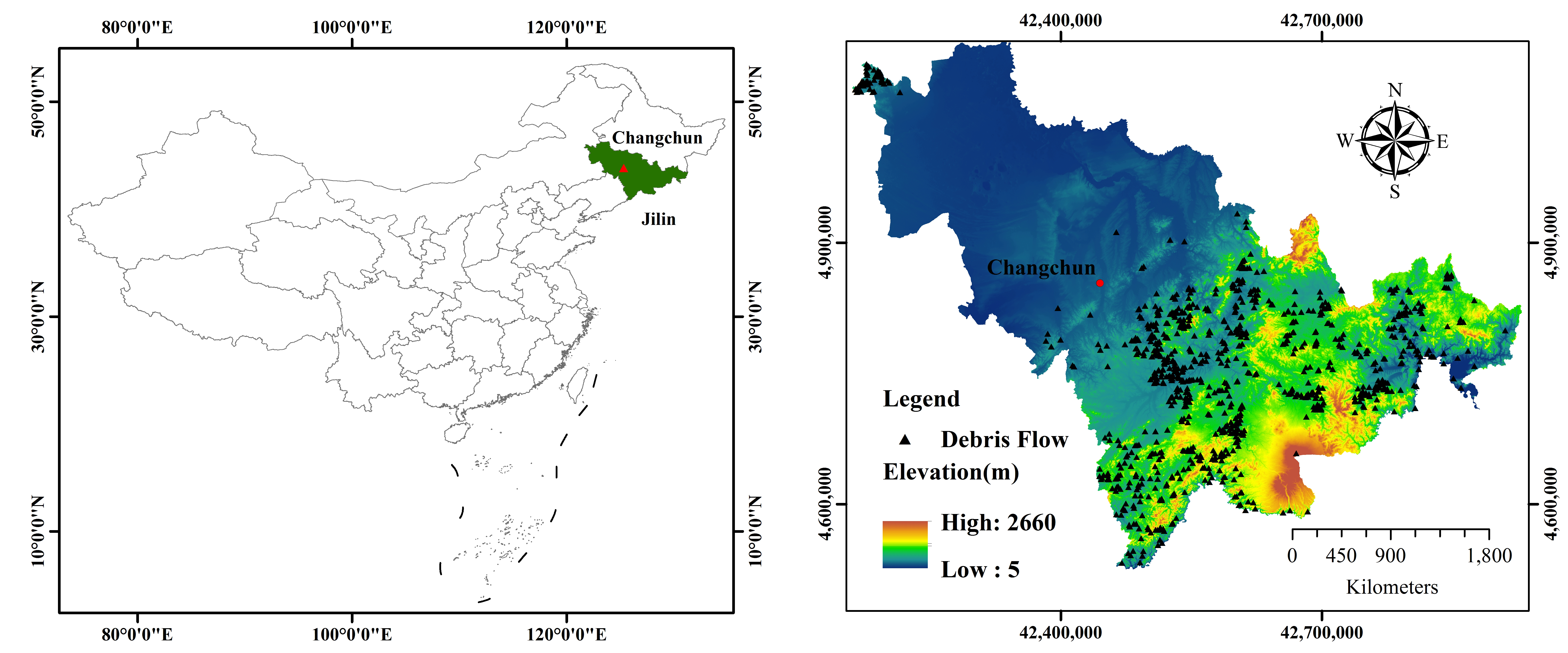
Figure 1. Location of study area and distribution of debris flow.
Water 12 02079 g001
Figure 2. The flowchart of the methodology used in this study.
Water 12 02079 g002
Figure 3. The one–dimensional corresponding relationship between thirteen influencing factor values and whether a debris flow occurs.
Water 12 02079 g003
Figure 4. One–dimensional to two–dimensional schematic.
Water 12 02079 g004
Figure 5. Debris flow influencing factors used in this study: (a) elevation, (b) slope, (c) aspect, (d) plan curvature, (e) profile curvature, (f) topographic wetness index (TWI), (g) distance to roads, (h) distance to rivers, (i) lithology, (j) population density, (k) annual rainfall, (l) topography, (m) vegetation coverage.
Water 12 02079 g005aWater 12 02079 g005bWater 12 02079 g005c
Figure 6. The LetNet–5 structure.
Water 12 02079 g006
Figure 7. The VALID padding convolutional neural network (V–CNN) structure and the procedure of debris flow data processing.
Water 12 02079 g007
Figure 8. The convolution manipulation (VALID padding).
Water 12 02079 g008
Figure 9. The subsampling manipulation (VALID padding).
Water 12 02079 g009
Figure 10. The SAME padding (S–CNN) structure and the principle and process of debris flow data processing.
Water 12 02079 g010
Figure 11. The convolution manipulation (SAME padding).
Water 12 02079 g011
Figure 12. The subsampling manipulation (SAME padding).
Water 12 02079 g012
Figure 13. Average merit (AM) values of influencing factors using the gain ratio (GR) method.
Water 12 02079 g013
Figure 14. Debris flow susceptibility maps: (a) 2D–CNN based on SAME padding (S–CNN), (b) 2D–CNN based on VALID padding (V–CNN), (c) Support Vector Machines (SVM), (d) Artificial Neural Network (ANN).
Water 12 02079 g014
Figure 15. The ROC curves and AUC values of the four models on the training set.
Water 12 02079 g015
Figure 16. The ROC curves and AUC values of the four models on the validation set.
Water 12 02079 g016
Figure 17. The mathematical statistics of the four models.
Water 12 02079 g017
Figure 18. The proportion of the prediction results of different models in the susceptibility level.
Water 12 02079 g018
Figure 19. Comparison maps of the susceptibility values of the four models: (a) comparison map of S–CNN and SVM, (b) comparison map of S–CNN and V–CNN, (c) comparison map of S–CNN and ANN, (d) comparison map of SVM and V–CNN, (e) comparison map of SVM and ANN, (f) comparison map of V–CNN and ANN.
Water 12 02079 g019
Figure 20. Relative importance of influencing factors to the four models.
Water 12 02079 g020
Table 1. Main geology and lithology in the study area.
SystemStratum CodeGroupMain Lithology
Archean eonAr1YangjiadianDark black, columnar structure, including plagioclase, hornblende, pyroxene
Ar2LaoniugouPyroxene granulite, hornblende metagranite, pyroxene magnetite rock
Proterozoic eonPt1LinjiangThe phyllite, sericite phyllite and diorite schist
Cambrian PeriodЄ1ChangpingGray medium–thin limestone, asphaltene limestone, dolomite limestone
Є2ZhangxiaBlue–grey bioclastic limestone, gray thin layered limestone
Є3GushanPurple siltstone, shale with thin limestone
Ordovician periodO1MajiagouLight gray dolomite limestone, flint nodular limestone
Silurian PeriodS1TaoshanGray, dark gray fine sandstone, siltstone, silty slate with mud limestone.
Devonian PeriodD2WangjiajieGray medium–thick layer limestone, bioclastic limestone
Carboniferous PeriodC2ShanxiDark coarse sandstone, siltstone, shale, and coal, with a thin layer of limestone
Permian periodP2SunjiagouRed mudstone, silty mudstone, and feldspar sandstone
Triassic PeriodT3DaxinggouVolcanic rocks with sedimentary clastic rocks and thin coal seams
Jurassic PeriodJ1HongqiSandstone, siltstone, mudstone
J2WanbaoSandstone, siltstone, carbonaceous mudstone
J3ShaheziGray sandstone, siltstone with five layers of coal
Cretaceous periodK1YaojiaInterlayer of brown–red mudstone and gray–green mudstone, siltstone
K2NenjiangMainly gray–black mudstone, with gray–green fine sandstone, siltstone
Tertiary periodE1FufengshanGray–green olive basalt, stomatal basalt, almond–shaped basalt
E2ShulanGray–green sandstone, siltstone, and mudstone coal seam
Quaternary periodQ1SihaiBlack basaltic volcanic slag and volcanic ash, black soil layer with clumps
Table 2. Database for influencing factors.
Influencing FactorsData TypeScale
ElevationGrid100 m × 100 m
SlopeGrid100 m × 100 m
AspectGrid100 m × 100 m
Plan curvatureGrid100 m × 100 m
Profile curvatureGrid100 m × 100 m
TWIGrid100 m × 100 m
Distance to roadsPolygon1:5,000,000
Distance to riversPolygon1:5,000,000
LithologyPolygon1:1,800,000
Population densityPolygon1:1,800,000
Annual rainfallPolygon1:5,000,000
TopographyPolygon1:1,800,000
Vegetation coveragePolygon1:1,800,000
Table 3. The meaning of each indicator in the receiver operative characteristic (ROC) curve.
TruePositive (Debris Flow)Negative (Non–Debris Flow)
Predicted
Positive (debris flow)TP (true positive)FP (false positive)
Negative (non–debris flow)FN (false negative)TN (true negative)
Table 4. The results of multicollinearity analysis.
Debris FlowCollinearity Statistics
Influencing FactorsToleranceVIF
TWI0.7531.328
distance to river0.9691.032
Vegetation coverage0.4762.099
topography0.5251.905
distance to road0.9881.013
lithology0.4892.047
population density0.9141.094
rainfall0.6871.455
profile curvature0.7881.268
plan curvature0.8411.19
aspect0.9921.008
slope0.6261.596
elevation0.7351.360
Table 5. The spatial relationship between influencing factors and debris flows by the frequency ratio (FR) method.
Influencing FactorsClassesPercentage of Domain (%,a)Percentage of Debris Flow (%,b)FR (b/a)
Elevation (m)<60075.68686.4061.142
600–80012.98313.0181.003
800–150010.9460.4610.042
>15000.3850.1150.299
Slope (°)<564.32353.6870.835
5–1015.33629.4931.923
10–2016.56815.4380.932
>203.7731.3820.366
AspectFlat11.0215.6450.512
North11.5328.7560.759
Northeast11.65511.1750.959
East11.07616.3591.477
Southeast11.34317.2811.524
South10.44313.0181.247
Southwest11.64412.5581.078
West11.0727.6040.687
Northwest10.2157.6040.744
Plan curvature (100/m)concave6.0107.2581.208
flat84.06085.0231.011
convex9.9307.7190.777
Profile curvature (100/m)<−0.312.2750.3460.152
−0.31–−0.107.9083.6870.466
−0.10–0.0672.62152.5350.723
0.06–0.2813.99536.8662.634
0.28–2.103.2016.5672.052
TWI<546.20850.8061.100
5–731.15121.0830.677
7–911.86410.8290.913
9–115.39611.8662.199
>115.3815.4151.006
Distance to roads (m)<10008.83012.2121.383
1000–20002.9662.8800.971
2000–30002.9823.4561.159
3000–40002.9901.6130.540
4000–50002.9992.3040.768
>500079.23377.5350.979
Distance to rivers (m)<5002.5763.3411.297
500–10002.0833.2261.549
1000–15001.9432.0741.067
1500–20001.8652.5351.359
2000–25001.8093.5711.975
>250089.72485.2530.950
LithologyGroup 146.54365.0921.399
Group 29.20921.1982.302
Group 31.85610.1385.462
Group 442.3923.5710.084
Population density (/km2)0–1010.4105.1840.498
10–10056.83570.3921.239
100–50032.54024.3090.747
>5000.2150.1150.536
Annual rainfall (mm)0–60072.08939.1710.543
600–80026.19260.5992.314
800–10000.8270.1150.139
>10000.8910.1150.129
TopographyPlain37.6330.4610.012
Valley6.31914.9772.370
Hills10.56512.4421.178
Mountains45.48372.1201.586
Vegetation coverageLow41.5337.1430.172
Moderate28.66355.4151.933
High18.62225.0001.343
Very high11.18212.4421.113
Table 6. Parameter settings of the CNNs.
MethodS–CNNV–CNN
Parameters
Number of iterations20002000
Convolutional kernel size3 × 33 × 3
Max pooling kernel size2 × 22 × 2
Activation functionReLUReLU
OptimizerAdamAdam
Dropout0.70.7
Learning rate0.00010.0001
The first full connection288288
The second full connection100100