Article

Numerical Study on Dynamical Structures and the Destratification of Vertical Turbulent Jets in Stratified Environment

1
State Key Laboratory of Hydrology-Water Resources and Hydraulic Engineering, Hohai University, Nanjing 210098, China
2
College of water Conservancy and Hydropower Engineering, Hohai University, Nanjing 210098, China
*
Author to whom correspondence should be addressed.
Water 2020, 12(8), 2085; https://doi.org/10.3390/w12082085
Submission received: 20 April 2020 / Revised: 28 May 2020 / Accepted: 21 July 2020 / Published: 23 July 2020
(This article belongs to the Special Issue Hydraulic Dynamic Calculation and Simulation)

Abstract

:
The law of pollutant emission and diffusion in stratified waters is a common issue. In this paper, numerical study on the interaction between vertical turbulent jets and the pycnocline is carried out to study the problems of jet’s emission through the large eddy simulation (LES). A trigonometric function disturbance (TFD) method is developed to ensure the velocity distribution of the jet in the horizontal plane yield to Gaussian profile. Numerical simulations are carried out in the range of 1.11 < Frp < 4.77, corresponding to 1393 < Rep < 5979, where the Froude number Frp and the Reynolds number Rep are defined at the entrance of pycnocline. The coherent structure and internal waves are observed at the pycnocline during the process of jets impinging. After the impingement, the destratification effects can be found. It can be found that Frp = 3 is a threshold value for the interaction between jets and the pycnocline. When Frp > 3, the interaction becomes intensely. Furthermore, the fitting formula of the radial momentum flux dissipation rate that is used to describe the decay of energy contained by the jets during the impinging process, is established through the dimensionless analysis. As a result, the influence range of the jet on the horizontal plane can be evaluated by Rep. It is also found that the destratification of jets is mainly affected by the velocity of the internal wave induced by jets. In addition, by employing the dimensionless time T related to that velocity, the law of destratification varies with dimensionless time is obtained, which can be summarized as follows: Due to the influence of the first internal wave, the thickness of the pycnocline increases rapidly and reaches a critical value at T = 1.4, after that, the increase of the thickness of the pycnocline becomes linear.

1. Introduction

The pollutant emission and diffusion in water environment is a common issue and these problems, such as the leakage of wastewater [1] and oil [2], can be generalized as the problems of jets [3]. In addition, the jet is also one of the motivations that cause the movement of fluid near jet’s trajectory, which may lead to the changes of water environment. For example, particles would be resuspended [4] with the influence of jets, which causes the changes of sedimentation in reservoirs and lakes [5]. As a result, there are many studies concerning properties of the jet in unstratified water. On the other hand, pycnocline can be commonly found in oceans, estuaries and lakes, normally produced by salinity or seasonal temperature stratification. The existence of stratification has many adverse effects on the water environment, such as substantial hypolimnetic oxygen depletion, which has a negative impact on aquatic systems and water quality [6]. Therefore, in stratified lakes and reservoirs with weak hydrodynamics, artificial destratification measures are often used to control stratification [7,8,9,10], mainly including underwater aeration [11] and mechanical disturbance [12]. However, the destratification of jets has not attracted people’s attention yet. Furthermore, the properties of jets in stratified water are quietly different from that in unstratified environment. Camassa [13] claimed that the rising height of the jet was affected by the density gradient, and it could not penetrate through the pycnocline if the momentum of the jet is not large enough. That is to say, the development of jets would be restricted by the pycnocline. So, it is necessary to study the interaction between jets and the pycnocline and it will provide reference for studying the emission law of pollutant and the destratification of jets.
Many studies indicated that the properties of jets in unstratified environment could be indicated by the values of some dimensionless parameters [14,15,16]. Turner [14] defined the initial density Froude number ( F r 0 = u 0 / r 0 g 0 , where the subscript ‘0′ refers to values at the source; u 0 is the vertical velocity of the jet; r 0 is the radius of the nozzle; g 0 is the reduced gravity), and studied the rise height of negatively buoyant fountains in the range of 0.55 < Fr0 < 11.8. The result indicated that the fountain stopped at the initial maximum rise height zm due to the negative buoyance. Then, the fountain fell back down around the up-flowing fountain core and settled at a steady-state height zs, and the rise height ratio λ = zm/zs ≈ 1.43. Burridge [15,16] studied the negatively buoyant fountain in the range of 0.4 < Fr0 < 45 and presented that the range of λ was 0.5~2.0. Furthermore, the negatively buoyant jet was divided into four classes: very weak, weak, intermediate, and forced.
With reference to dimensionless parameters of jets in unstratified water, researchers also defined some parameters to study jets in the stratified environment. Ezhova [17] defined the Froude number before the jet reaching the pycnocline F r t = 0.5 U max / R t g , where Umax and Rt are the maximum velocity and the radius of the jet at the entrance to the thermocline, and studied the penetration height of jets under stratified environment in the range of 0.6 < Frt < 1.89 by both experimental and numerical simulation. Druzhinin [18] defined the Froude number of the jet as Fr = w0/N0D0, (where w0 is the initial velocity of the jet; D0 is the nozzle diameter of the vertical jet; N 0 = g ρ 0 Δ ρ D 0 is the buoyancy frequency at the center of the pycnocline; ρ 0 is the density at the center of the pycnocline; Δ ρ is the density difference between upper and lower layers) and studied the interaction between jets and the pycnocline by DNS.
The interaction between jets and the pycnocline is studied based on the parameters mentioned above. During the rising process, the density of the jet at the pycnocline entrance is equal to the density of lower layer due to the jet entrains the surrounding fluid [17]. After the jet penetrates the pycnocline, the momentum of the core of upward flow rapidly decays due to negative buoyancy when the jet penetrates through the pycnocline. Then the jet falls back and impinges on the pycnocline after reaching the maximum penetration height. As a result, internal waves are generated at the pycnocline [19,20,21,22]. Figure 1 is the schematic diagram. Ezhova [19,20,21] compared the theoretical results based on the conservation of energy with the LES results and indicated that the theoretical penetration height was related to F r t 2 , but the penetration height was overestimated at the largest Frt because turbulence during the entrainment was not taken into account. Cotel [22] analyzed the entrainment and the coherent structure after the jet penetrated into the upper layer. It was found that with the effect of the shear force caused by the counterflow of the jet, vortices with opposite directions were formed in pair on both sides of the pycnocline. Druzhinin [18] indicated that the jet maintained a stable state after breaking through the pycnocline when the Froude number was less than 2. However, when the Froude number was greater than 2, the jet began to oscillate, which would be accompanied by the generation of internal waves.
The phenomenon of the jet penetrating the pycnocline is similar to the scheme of the bubble plume that is usually applied to destratification. Mcdougall [23] first put forward the double plume model of bubble plume in a stratified environment. Kim [24] studied the relationship between bubble size, diffusing area, and de-stratification efficiency through physical experiments. Destratification of a single-phase buoyant jet is similar to bubble plume. Neto [25] compared bubble plume with single-phase plume and indicated that bubble plume also generated a fountain at the pycnocline. In addition, the height of fountain and entrainment properties of the bubble plume were also similar to the single-phase plume, and the generation of internal waves could be seen from the experimental results. Therefore, it is necessary to research the destratification of single-phase jet.
In this study, a three-dimensional (3D) LES model is established to study the interaction between vertical jets and the pycnocline and the destratification effects of jets. The research is carried out with the following three aspects: (1) Analyzing the impingement process and coherent structure of the jet under stratified environment; (2) obtaining hydraulic properties of interaction between jets and a pycnocline; (3) developing destratification function of jets. In Section 2, the numerical models together with the TFD method are introduced. In Section 3, verifications and parameters of the model are introduced. In Section 4, the simulation results are discussed. The results of this study can provide theoretical basis for hydraulic and entrainment properties during the emission of pollutants in the stratified environment.

2. Governing Equations and Numerical Methods

2.1. Model Description

As shown in Figure 2, a 3D numerical model is established to study hydraulic properties of the interaction between a vertical jet and a pycnocline. The size of water tank is 1 m × 1 m × 0.5 m in x, y and z direction respectively. The non-uniform grid system is adopted to save computation costs. As shown in Figure 3, the whole computational domain is discretized into 100 × 100 × 80 nodes, and the time step is 0.001 s corresponding to the grid scale. Due to the inaccuracy in simulating the round nozzle with rectangular grid, a rectangular nozzle is adopted instead, which is also used by Chen [26]. The nozzle (width L0 = 0.88 cm) is located at the center of the bottom in the stratified environment. The velocity of jets in our cases is in the range of 0.2 m/s to 1.0 m/s. The pycnocline is located at z = 0.25 m. ρu and ρd are the density of upper and lower layers, respectively. hu and hd are the height of the upper and lower layers, respectively. The density of the jet is the same as that of the lower layer.
The dimensionless nozzle size is 0.0088 that is calculated by the width of nozzle and the horizontal size of the computational domain. There are many references about the horizontal dimensionless nozzle size both in numerical simulations and experiments. Table 1 shows the comparison of the dimensionless nozzle size between previous researches and this study. It can be found that the dimensionless nozzle size is suitable in this paper.

2.2. Governing Equations

The 3D, unsteady, incompressible, filtered continuity and Navier–Stokes equations (NSEs) with the Boussinesq approximation in rectangular coordinates are written as:
Continuity equation:
u ¯ i x i = 0
Momentum equations:
u ¯ i t + u ¯ j u i ¯ x j = 1 ρ a p ¯ x i + x j ( ν u i ¯ x j τ i j ) + ( ρ ρ a ) g i
Scalar transport equation:
c ¯ t + ( u ¯ j c ¯ ) x j = x j [ ( α + α t ) c ¯ x j ]
where the subgrid Reynolds stresses τ i j = 2 ν t S i j ¯ = ν t ( u ¯ i x j + u ¯ j x i ) , the turbulent viscosity coefficient ν t = ( C s Δ ) 2 2 S i j ¯ S i j ¯ , the Smagorinsky coefficient Cs is taken as a constant in this study and Cs = 0.10, Δ = ( Δ x Δ y Δ z ) 1 3 . gi is the gravitational acceleration; ρ a is the density of the ambient water; the molecular diffusion coefficient α = ν P r ; the turbulent diffusion coefficient α t = ν t P r t . In this study, the Prandtl Number (Pr) and the turbulent Prandtl Number (Prt) are set to 0.7 and 0.3, respectively.
The fluid density ρ is related to the scalar concentration, which can be given by:
ρ = ρ 0 + β c
where ρ0 = 998 kg/m3 (pure water); β is the concentration contraction coefficient; and c is the concentration.

2.3. Numerical Methods and Boundary Conditions

An operator splitting method is used to solve the governing equations mentioned above. At each time step, the flow equations are split into three steps: advection, diffusion and pressure propagation steps, while the transport equation is split into two steps: advection and source steps. In this study, a combination of the Lax-Wendroff and the quadratic backward characteristic methods is employed to solve the flow advection. The central difference method is used to discretize the diffusion step. The projection method is used with the help of the continuity Equation (1) to solve the additional terms, including the pressure and the gravitational forces in the NSEs. A stable and robust conjugate gradient stabilized method (CGSTAB) is employed to solve the Poisson pressure equation. The details of the numerical method are to be found in Zhu’s [28] and Lin’s [29] study.
Zero gradient condition is adopted at the wall of the tank, and sponge boundary [30] with a thickness of 10 cm is imposed near the wall in order to reduce the influence of the wall. Rigid lid assumption is used on the free surface due to the jet is far enough from the surface. No slip boundary condition is adopted at the bottom of tank. Initial condition is a stable stratified water environment. The vertical velocity distribution of the jet is given by top-hat function:
w 0 ( x ) = w 0 [ 1 ( x 2 L 0 2 ) 3 ]
where w0 is the initial velocity of the jet; x is the coordinate defined by Figure 2; L0 is the initial width of the jet.
It is necessary to add disturbance at the jet inlet boundary in order to simulate turbulence characteristics of jets. A trigonometric function disturbance (TFD) method is developed based on S.Menow’s [31] azimuthal forcing method. Compared with S. Menow’s azimuthal forcing method, a random angle θr and an extra cosine function are employed in the TFD method to ensure velocity distribution of the jet in the horizontal plane yield to Gaussian profile. The disturbance formulas are written as follows:
u = A u w 0 ( r ) n = 1 N sin ( 2 π f t / n + θ r )
v = A v w 0 ( r ) n = 1 N cos ( 2 π f t / n + θ r )
where Au and Av are the amplitudes of fluctuation in x and y direction, respectively; θr is the random angle varying from 0 to π with time; N is the number of modes (set to 6); f is the frequency determined by the jet preferred mode corresponding to a Strouhal number. Strouhal number of the jet is roughly between 0.2 and 0.8, thus, in this study Strouhal number is set to 0.3.
Although employing the azimuthal forcing method can achieve ideal vertical velocity decay of jets by several scholars [32,33], the velocity distribution of the jet in the horizontal plane is difficult to yield to the Gaussian distribution. Because only sine function is used in azimuthal forcing method which causes the correlation between u and v. After applying the TFD method, there is a difference with a period of π/2 in disturbances between the x and the y directions. Therefore, it can be guaranteed that the u and v components of the jet velocity are uncorrelated. In order to compare the traditional azimuthal forcing method with the TFD method, the u and v at the plane of Z = 20 from the results simulated through two methods are extracted and a plot of the values of u/wc and v/wc is shown in Figure 4. It can be seen that the points obtained through the TFD method distribute randomly in the uv plane, while the points obtained through the traditional azimuthal forcing method almost make up a line of u = v, namely the u and v are uncorrelated by employing the TFD method.
In addition, the comparisons between the results simulated via the azimuthal forcing method and the TFD method are shown in Figure 5. It can be observed that the profiles of vertical velocity and concentration simulated through the TFD method are better yield to Gaussian profile than that simulated through azimuthal forcing method. More validations can be found in Chapter 3.

2.4. Dimensionless Description

Dimensionless numbers in this study are defined as follows:
R = r / L 0 ,   ( X , Y , Z ) = ( x , y , z ) / L 0 ,   ( U , V , W ) = ( u , v , w ) / w 0 H = h / L 0 ,   H c = h c / L 0 ,   P i = p i / L 0 P s = p s / L 0 ,   R inf = r inf / L 0 ,   T = c w t / r g
where L0 is the width of the nozzle; u, v, and w are velocity components in x, y, and z directions; h is the initial pycnocline thickness; hc is the critical pycnocline thickness; pi is the initial penetration height of jets; ps is the stable penetration height of jets; rinf is influence range of jets in horizontal direction; cw is the velocity of the first internal wave produced by the jet; rg is the radial distance from the observation point to the axis of jet, in this study rg is set to 0.3 m.
Druzhinin [18] claimed that jet dynamics were governed by the values of the Froude Number and Reynolds number. Burridge’s [15] study indicated that the nozzle size and the velocity of the jet could be described through the dimensionless Froude Number and Reynolds number. In order to extend our model to the real scale in the stratified environment, the Froude number and Reynolds number at the entrance of pycnocline, which are based on the characteristics of jets and the pycnocline, are defined as follow:
F r p = 0.5 w c p / r p g
Re p = w c p r p v
where g = g Δ ρ / ρ 0 is one of the characteristics of the stratified water environment; ρ 0 is the density of the upper layer; Δ ρ is the density difference between upper and lower layers; w c p is the velocity of jet axis at the entrance to the pycnocline; r p is the half-width of jets at the entrance to the pycnocline. w c p and r p represent the properties of jet at the entrance of pycnocline.
In addition, the initial Froude number and Reynolds number of jets at the source is defined as:
F r 0 = w 0 / L 0 g
Re 0 = w 0 L 0 v
where w0 is the initial vertical velocity of jets; L0 is the width of the nozzle.

3. Model Validation

Numerical cases are detailed in Table 2. Cases A0 and A1 are used for validation. Cases A1~A9 are the jets with different momentums and same initial pycnocline thickness. These cases are used to study the hydraulic properties of the vertical turbulent jets interacting with the pycnocline. The velocities of jets in cases B1~B2 and B3~B4 are 0.5 m/s and 0.8 m/s, respectively. While the dimensionless initial thicknesses of the pycnocline in cases B1, B3 and B2, B4 are 2 and 4, respectively. Cases B1~B4 are used to study the destratification effects of jets.

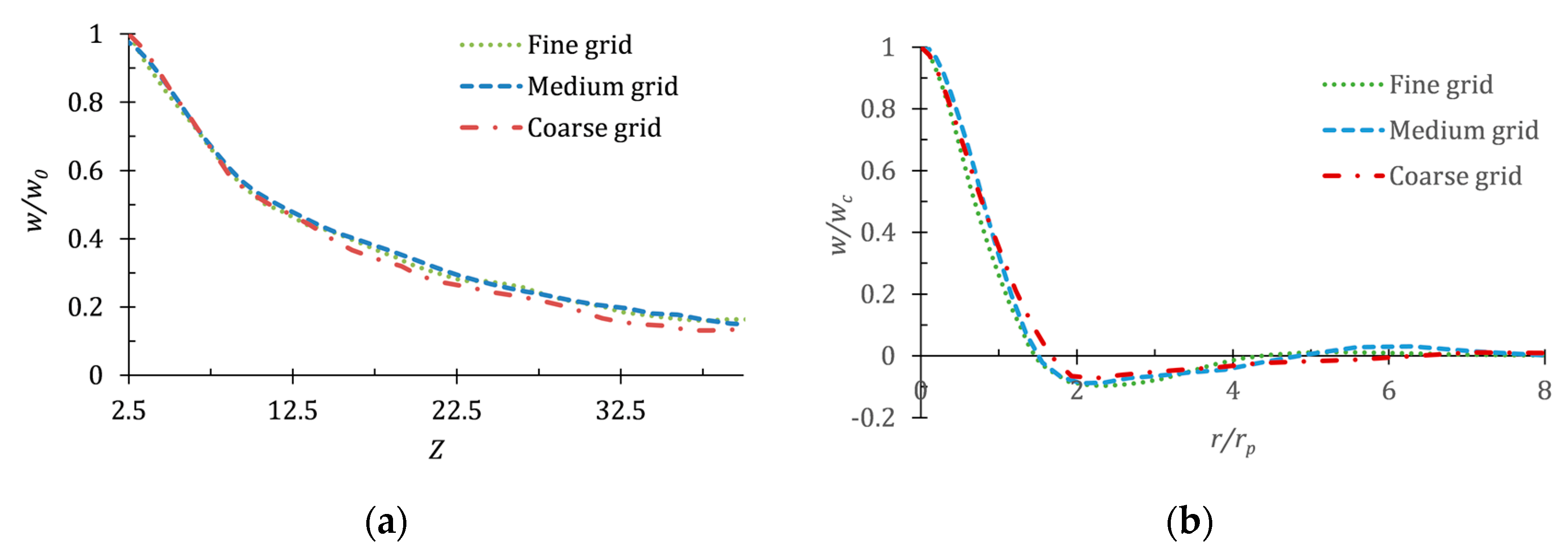
3.1. Mesh Refinement Study

To illustrate that the grid size used in this paper does not affect the calculation results, cases A0 and A9 are separately simulated by a coarse grid system (80 × 80 × 60) and a fine grid system (150 × 150 × 110). The comparisons between these two grid systems with medium grid system (100 × 100 × 80) which is adopted in the verification are shown in Figure 6. As shown in Figure 6a, the vertical velocities at the jet axis in three different grid systems have little differences. It proves that the medium grid size can accurately simulate the jet. As shown in Figure 6b, the vertical velocity profiles of jets at the pycnocline in fine and medium grid systems have little differences. It proves that the medium grid size can accurately simulate the interaction between jets and the pycnocline.
In our model, the courant (CFL) number in all three directions are controlled to be less than 1.0. The CFL number in X, Y, and Z directions are defined as follows:
C F L x = Δ t u Δ x ,   C F L y = Δ t v Δ y ,   C F L z = Δ t w Δ z
The initial time step is set to 0.001 s in our model, and the maximal velocity is 1.0 m/s at the jet nozzle, and the minimum grid size is 0.0011 m at the jet nozzle. It can be estimated that the maximum CFL number is about 0.9 in our model. Furthermore, the dynamic time step method is used in our LES code to avoid CFL exceeding the threshold value, namely 1.0. If the CFL number is larger than 1.0, sub-steps (Δt1) will be employed for computation automatically instead of the original time step Δt. In addition, case A9 is chosen to analyze the CFL number. Figure 7 shows the mean CFL number varying with Z at the central line of the jet. It can be found that the CFL number is always less than 1.0.

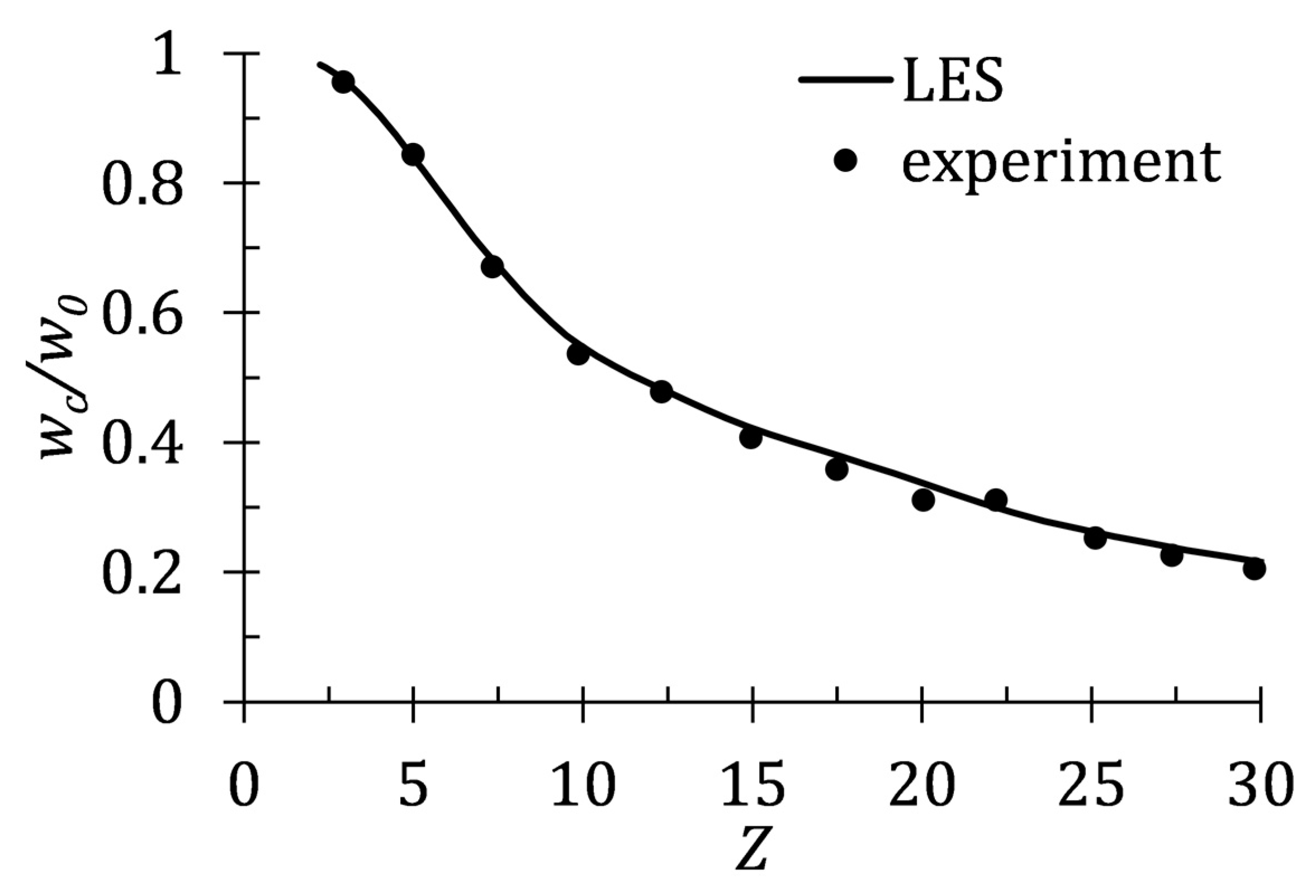
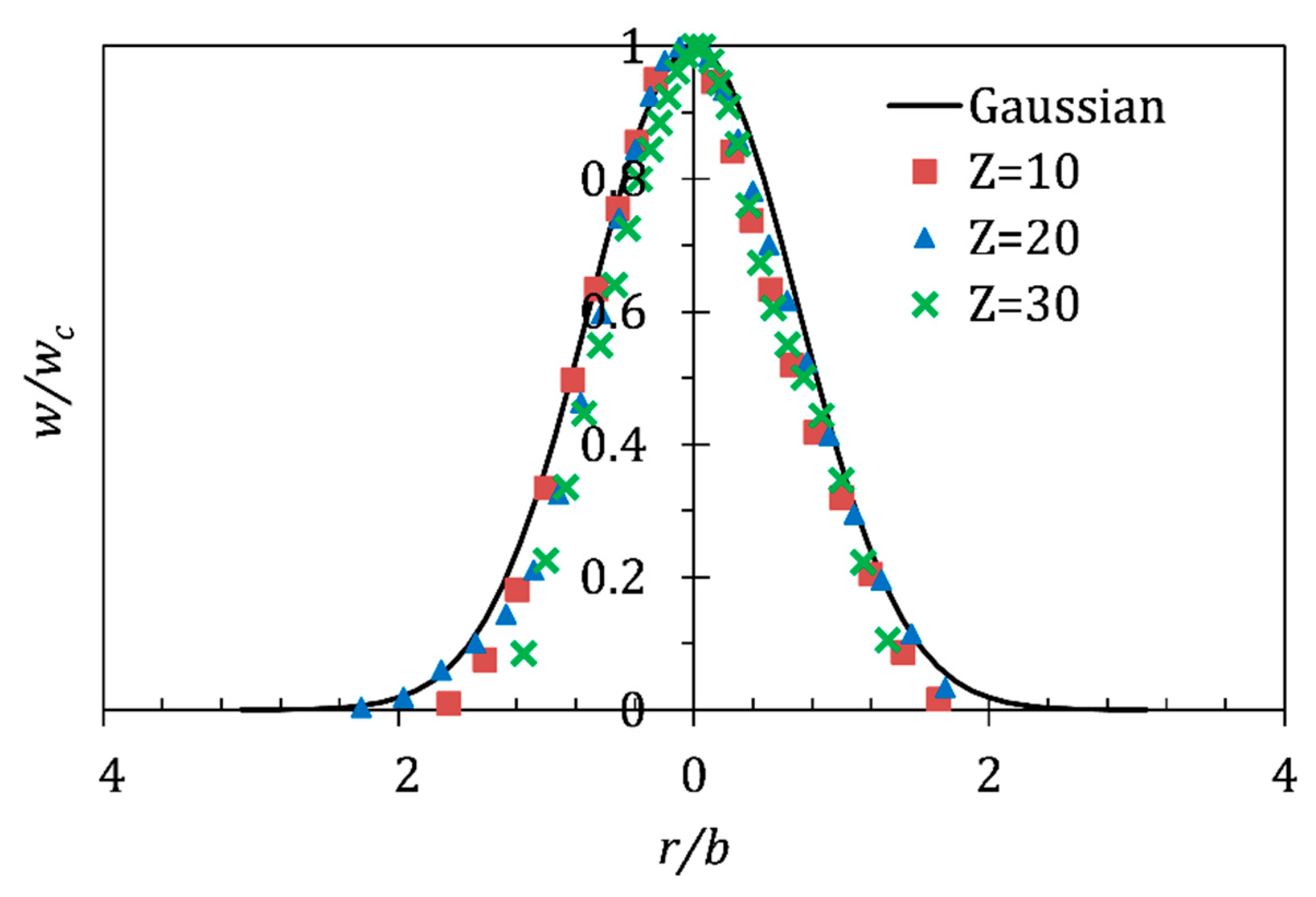
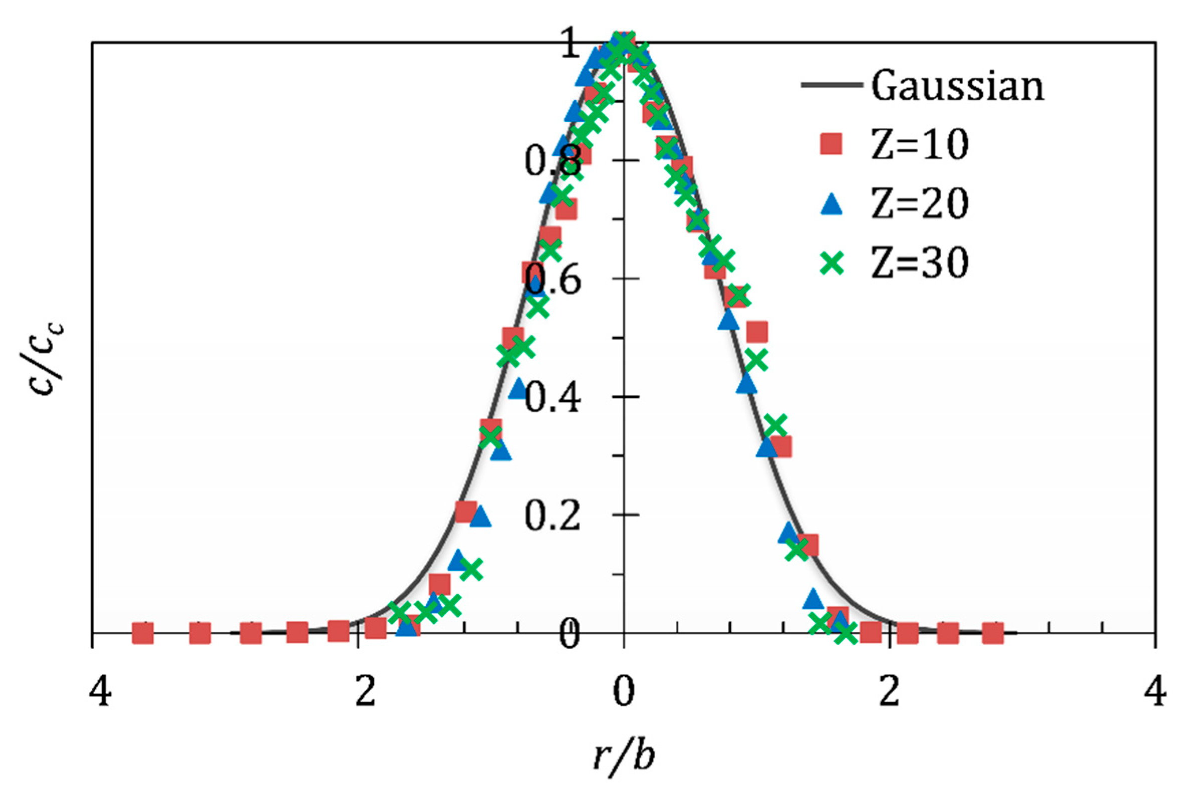
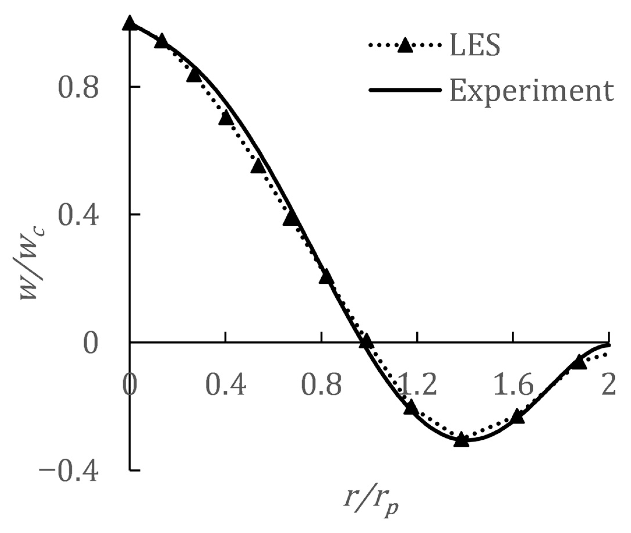
3.2. Validation for the Turbulent Jet in a Unstratified Fluid

In order to validate the fully developed jet adopting the TFD method, a case (A0) of a turbulent jet in a homogeneous fluid is carried out and mean vertical velocity are compared with the result of Xu’s laboratory experiments [34]. The size of computational domain and the number of grids are described in Section 2.1. The initial velocity of the vertical jet at the bottom is 0.88 m/s, and the jet density is the same as the environment fluid. A numerical concentration contained by the jet is initially set as 10 mg/L to trace the jet trajectory, which actually, has no effects on the fluid density.
Figure 8 shows the comparison between numerical results and experimental results of Xu’s work. It can be seen that the decay of the axial vertical velocity of the jet in the LES is in good agreement with Xu’s experimental results.
The profiles of the velocity and concentration of the jet in horizontal plane yield to the Gaussian distribution:
w w c = exp [ ( r b ) 2 ]
c c c = exp [ ( r b ) 2 ]
where wc is the vertical velocity of jet axis; cc is the concentration of jet axis, b is the half width of the jet.
Numerical concentration and velocity of Z = 10, Z = 20, Z = 30 are extracted for verification. As can be seen from Figure 9 and Figure 10, the velocity and the concentration distribution are close to Gaussian distribution.

3.3. Validation of the Jet in a Stratified Fluid

The laboratory experiment of a vertical jet in a stratified environment by Ezhova [21] is adopted to verify the development of the jet in the stratified environment in our model. The Frp of case A1 is the same as that of the laboratory experiment; thus, case A1 is used to verify the vertical velocity profile of the jet at the pycnocline. Comparison of the result from the LES model (Frp = 1.11) with the vertical velocity at the thermocline from the experiment of Ezhova and Troitskaya is shown in Figure 11.

4. Results

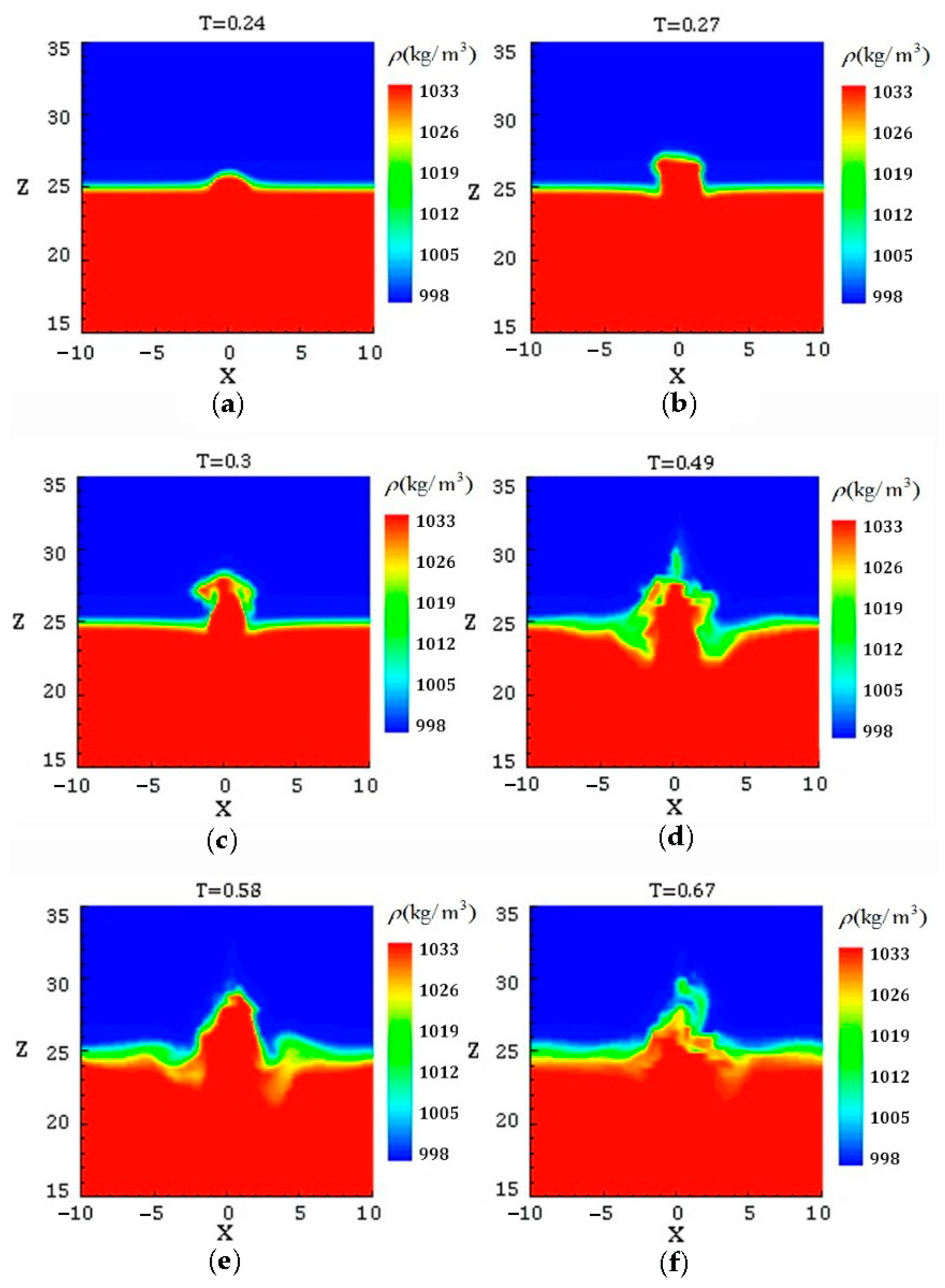
4.1. The Process of Impingement

As shown in Figure 12, the process of the interaction between the jet and the pycnocline, and the generation of internal waves are illustrated by the instantaneous fields of density during T = 0.24~0.67 in case A3. When the jet penetrates into the upper layer at dimensionless time T = 0.24, a domelike structure is formed at the top of the jet. Meanwhile, the jet does not break up and there is no obvious vortex at the pycnocline. Then at T = 0.27, the vertical velocity at the top area of the jet decreases to 0 due to the negative buoyance, but the core of the jet below the top area still retains some momentum and keep rising. Then at T = 0.3, part of the fluid falls back from the top of the jet, and core of the jet rises to its highest level before complete collapse. This level is defined as the initial penetration height Pi in this study. When T = 0.49, the jet collapses, and the counterflow penetrates into the lower layer under the action of momentum, which causes a sag generated at the pycnocline around the jet. Meanwhile, the pycnocline around the jet becomes thick with the influence of turbulence. At T = 0.58, the pycnocline around the jet bounces back and internal waves generated during this process. According to the last contours of Figure 12 at T = 0.67, the pycnocline settles after the internal wave propagates far away. The pycnocline becomes thicker compared with that at T = 0.24~0.3. Subsequently, a fountain, which oscillates up and down around a certain level, is formed as a result of the interaction between the jet and the pycnocline. Thus, the mean penetration height is a constant value defined as stable penetration height Ps. The schematic of the comparison between the initial penetration height Pi and the stable penetration height Ps is shown in Figure 13, and the penetration height is further analyzed in Section 5.1.

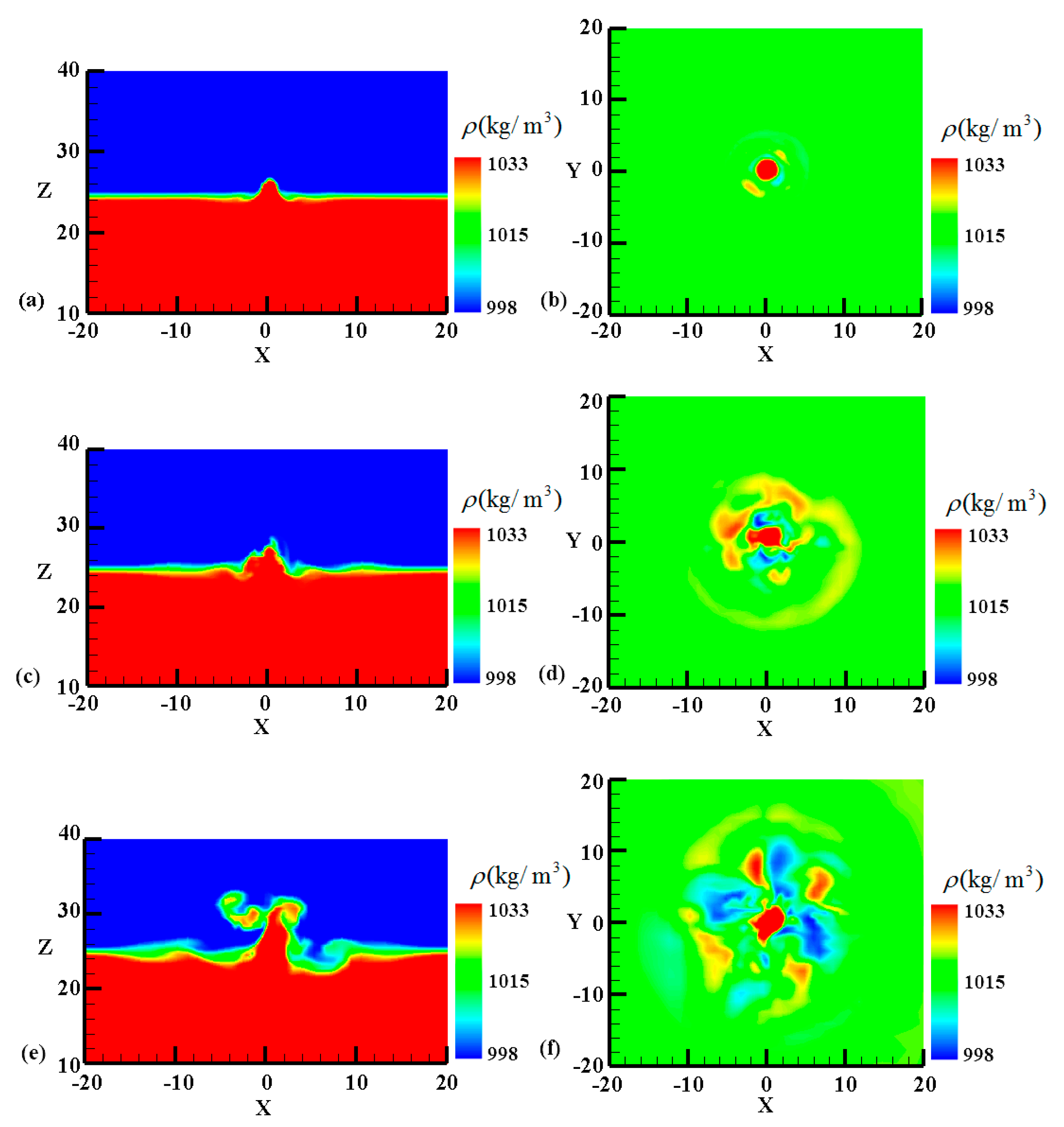
4.2. Generation of Coherent Structures.

The coherent structures caused by the interaction between the jet and the pycnocline directly affects the diffusion characteristic of the jet. These coherent structures are illustrated by the instantaneous fields of density at dimensionless T = 0.6, which are shown in Figure 14. The first observation is that the greater the Frp is, the greater the degree of jets’ breaking up is after penetrating through the pycnocline. It can be also found that the greater the Frp is, the higher the jets penetrate into the upper stratification layer. In addition, the counterflow is more evident with the increasing Froude number. As a result, more obvious internal waves are generated under the influence of the counterflow impinging on the pycnocline. In the case A1 with the minimum Frp, the jet does not break up after penetrating through the pycnocline, and no internal waves are generated. In the case A3 with a greater Frp, although the jet breaks up after penetrating through the pycnocline and internal waves are generated, the turbulence is not strong and the amplitudes of internal waves are small. In the case A9 with the largest Frp, the jet flow has a more complicated structure, in the meanwhile, strong turbulence and internal waves with large amplitude are generated.
To quantify the coherent structures illustrated above, we calculate the turbulent kinetic energy ( q = ( u 2 + v 2 + w 2 ) / 3 ) of five observation points at (±2, 0, 26), (0, ±2, 26), and (0, 0, 26) after jets penetrate through the pycnocline. Figure 15 shows the sum of turbulent kinetic energy at five observation points in each case. According to the turbulent kinetic energy, we can divide the intensity of the interaction between the jet and the pycnocline into four classes. (1) No turbulence. When Frp is small enough such as the case A1 (Frp = 1.11), the jet does not break up after penetrating through the pycnocline and the turbulent kinetic energy is close to 0. (2) Weak turbulence. Jets begin to break up after penetrating through the pycnocline. Such as cases A2~A4 where Frp is in the range of 1.37 to 2.83. Linear regression is used to fit the increase of q with the growth of Frp. The slope of the fitting line is only 0.015 and the turbulent kinetic energy maintains at about 0.1 which means that the increasing rate of q is very slow in these cases. The reason for this phenomenon is that the turbulence caused by the interaction between jets and the pycnocline is not strong enough. (3) Intermediate. In cases A5 (Frp = 3.19) and A6 (Frp = 3.66), the change of turbulence energy experiences an obvious increase. (4) Intense turbulence. When Frp is large enough, the jet completely breaks up due to the interaction with the pycnocline. Such as cases A7~A9 where Frp is in the range of 4.07 to 4.77. The growth law of q in this class is similar to Class 2. The slope of the fitting line is 0.014 and the turbulent kinetic energy maintains at about 0.2. It is because that the turbulence already reaches its most intense state, thus the turbulent kinetic energy can not increase any more.
For further studying on the coherent structure caused by the interaction between the jet and the pycnocline, Ω-vortex identification method proposed by Liu [35] is used to draw 3D coherent structures. The instantaneous coherent structures of case A6 are shown in Figure 16. From the streamlines in Figure 16a, it can be seen that the jet cannot penetrate through the pycnocline completely. Part of fluids penetrates through the pycnocline, and falls back to the pycnocline again. Hence, vortices are formed on the upper of the pycnocline by the shear force due to the horizontal flow. The other part which is blocked by the pycnocline also causes vortices formed under the pycnocline. As a result, vortices with opposite directions are formed in pair on both sides of the pycnocline, and the coherent structure is shown in Figure 16b.

4.3. Destratification of Jets

In order to illustrate the destratification of jets, the thicknesses of the pycnocline at about 60 s after impingement are extracted and the average of the dimensionless thicknesses ( Δ H ¯ ) are calculated from R = 15 to R = 35. Figure 17a shows variations of Δ H ¯ with Frp in cases A1~A9. According to Figure 17a, the thicknesses of pycnocline in all cases obviously increase with the influence of jets, which proves the destratification of the jet. It can be also found that the destratification effects have little differences when Frp < 3, however, the destratification effects obviously increase when Frp > 3. Figure 17b shows the distributions of the pycnocline thickness in cases A3, A6, and A9. The changes of ΔH are small between the different R, thus it is reasonable to use Δ H ¯ regardless of variation of R to illustrate the destratification of jets. In addition, the destratification effect can be observed in a wide range around the jet.

5. Discussions

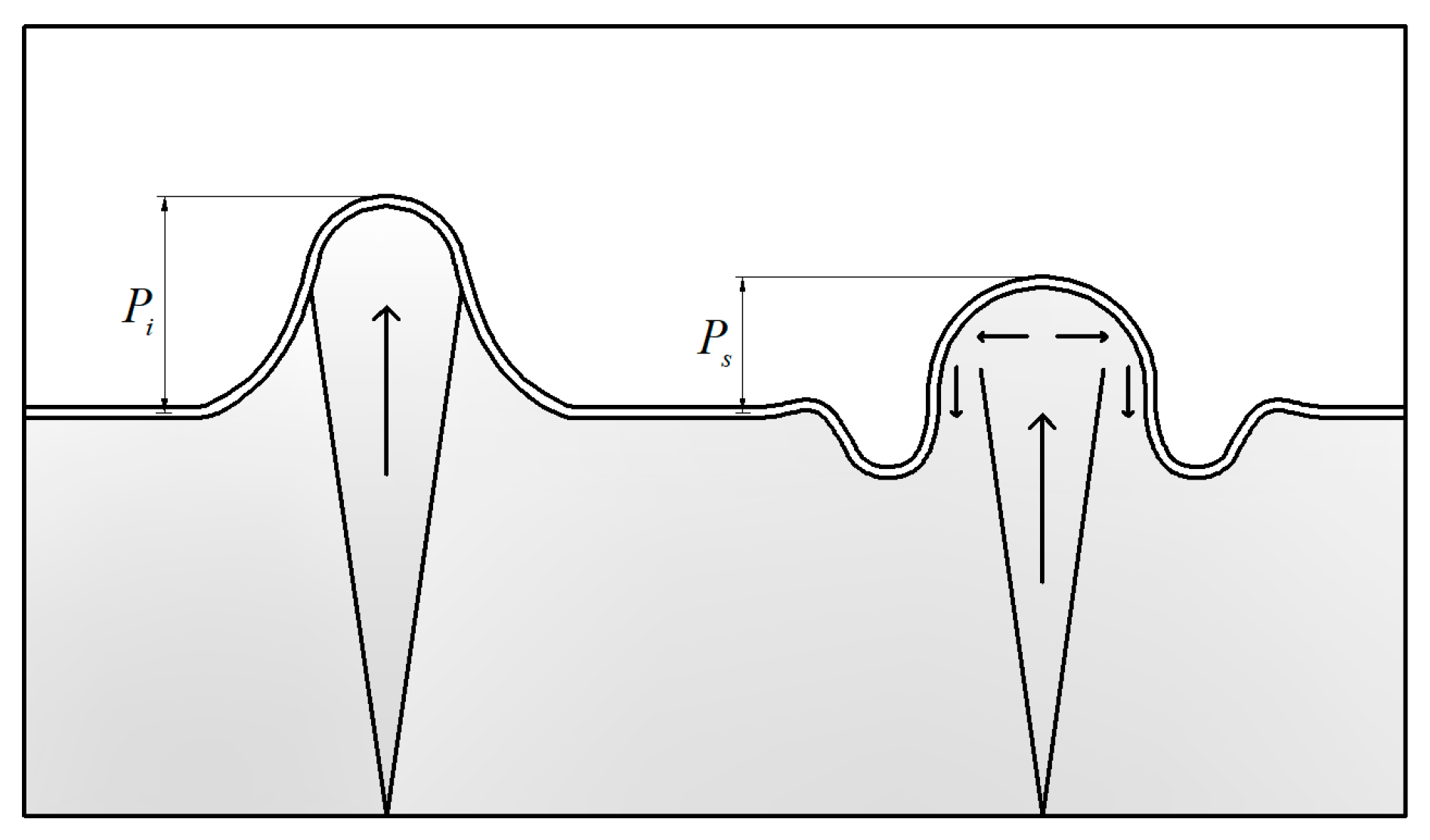
5.1. Quantitative Analysis of Hydraulic Properties of Jets Around the Pycnocline

The hydraulic properties near the jet impinging site at the pycnocline are discussed quantitatively in this section including the penetration height and momentum flux dissipation rate due to those properties directly affect the diffusion of jets around the pycnocline.
The initial penetration height Pi and stable penetration height Ps mentioned in Section 4.1 are defined referred to the penetration height of the buoyant jet in the unstratified environment. The later one has been well studied at present. The radial dynamical characteristic near the pycnocline is also different from that in an unstratified environment due to the influence of the interaction between jets and the pycnocline. In order to identify how far the jet can affects at the horizontal plane around the pycnocline, the radius of the region where the radial velocity (ur) is greater than 1% of the initial velocity of the jet is defined as the horizontal influence radius Rinf.
Figure 18a shows the relationship between dimensionless penetration height and Frp. The results indicate that Pi increases linearly with the growth of Frp when Frp < 3, and Pi/Ps is around 1.4 which is similar to the experimental results of Turner’s [14] and Hunt’s [15] studies, despite their studies in the unstratified fluid. When Frp > 3, the value of Pi oscillates irregularly because the momentum of jets before impinging on the pycnocline is large, as a result, the collapse of jets occurs at different speeds after jets penetrate through the pycnocline. While Ps still increases linearly. Figure 18b shows the relationship between the dimensionless horizontal influence radius Rinf and Frp. When Frp < 3, the value of Rinf is very small and increasing slowly with the growth of Frp. However, Rinf increases rapidly when Frp > 3, in other words, the jet has a greater effect on the disturbance of the surrounding water at the pycnocline.
Both the results of initial penetration height and the horizontal influence radius indicate that Frp = 3 is a threshold value, and that when Frp > 3 the turbulence caused by the interaction between the jet and the pycnocline becomes larger. This turbulence also causes the dissipation of jets’ momentum. Using mean data to calculate the momentum flux dissipation rate Kd of the jet, the expressions are written as follows:
K d = 1 F L h 20 F L j e t = 1 Z 1 Z 2 2 R ρ U U r d z 0 ρ U w r d r
where FLh20 is the radial momentum flux at R = 20 (where the pycnocline is not affected by the strong turbulence caused by the fountain). In this study, Z1 and Z2 are 15 and 35, respectively. FLjet is vertical momentum flux of the jet at Z = 19 (where the jet is not obviously affected by the pycnocline); U is the velocity; Ur is the radial velocity of the jet.
Figure 19 shows the relationship between Kd and Frp. It shows that Kd increases with the growth of Frp before Frp reaches 3. After Frp = 3, Kd becomes stable around 0.9. It claims that the turbulence becomes strong after Frp = 3, therefore, the momentum of jets decay rapidly. The mentioned results further prove that Frp = 3 is a threshold value for the interaction between jets and the pycnocline.
The mean data is used to calculate the radial momentum flux dissipation rate with Kh = FLh/FLh5 (Where FLh is the radial momentum flux; FLh5 is the radial momentum flux at R = 5). The radial momentum flux is calculated with an interval of R = 2.5 in the range of R = 5~30. The distribution of radial momentum dissipation is shown in Figure 20. In cases A1~A3, the tendency of the radial momentum dissipation rate is not obvious due to the weak hydraulic properties. However, for cases A4~A9, the exponential function is used to fit the calculation results of A4~A9, and the regression formula is:
K h = 0.19 + 1.25 e 250.88 R 5 Re p ,   3500 < Re p < 6000
where the Reynolds number at the entrance of pycnocline in this study is defined as Re p = w c p r p / v , and it is detailed in Section 3.

5.2. Quantitative Analysis of the Destratification of Jets

As illustrated in Section 4.1, pycnocline becomes thick with the influence of internal waves generated by the jet. Furthermore, the growth of pycnocline thickness H with the variation of time is analyzed in this section. In order to link the destratification with internal waves generated by jets, the time t is standardized by employing velocity of the first internal wave generated by the jet during the impingement. The definition of the dimensionless time T is detailed in Section 2.4.
Only cases A3~A9 are chosen to study the destratification effect of jets, as there are no obvious internal waves in cases A1 and A2. Furthermore, the destratification effects of jets with different initial pycnocline thickness are studied through cases B1~B4. The average thickness of four points (X = ± 30, Y = 0; X = 0, Y = ±30) is measured as the thickness of pycnocline at R = 30.
Figure 21 shows the relationship between the thickness of the pycnocline at R = 30 and the dimensionless time T. The change processes of the thickness can be divided into two stages. The first stage is T < 1.4. The pycnocline is stable when jets are far away from the pycnocline. When T = 1, the first internal wave reaches R = 30, and the thickness of the pycnocline begins to increase obviously with the influence of internal waves. Then (T = 1.4), the thickness of the pycnocline approaches to a certain value with the effect of the first internal wave. We define this value as the critical thickness Hc, and the critical thickness in different cases are very close. Even in the cases with the largest initial pycnocline thickness, Hc is a little bit thicker than the cases with small initial pycnocline thickness. The second stage is T > 1.4, the increasing rate of the thickness slows down, and the process tends to be linear. The reason is that the influence of internal waves on the thickness of the pycnocline becomes smaller when the pycnocline thickness is larger than critical value. The relationship between the H and T in the range of 1.4 < T <6 is fitted only through cases A3~A9 while cases B1~B4 in which the T only ends at 4 are used for further testing. The fitting formula is shown as follows:
H = 1.06 T + 3.27
where H = h / L 0 is the dimensionless thickness and T = c w t / r g is the dimensionless time as defined in Section 2.4.
Nash–Sutcliffe efficiency coefficient (donated as Ens below), which is widely used to evaluate the performance of hydrological model, is employed to evaluate the performance of the fitting line Equation (18) in different Frp. The definition of Ens is shown as follows:
E n s = 1 i = 1 n ( S i F i ) 2 i = 1 n ( S i S ¯ ) 2
where Si is simulated value; Fi is fitted value; S ¯ is the average of simulated values. The result of Ens varying with Frp is shown in Figure 22.
It can be found that Ens in all cases are larger than 0.5, which represents the good performance of the fitting line [36], despite that the results of B1~B4 are not used for fitting. Thus, the fitting formula can be extended to the cases with different initial pycnocline thicknesses. However, Ens is relatively small in the cases with the largest initial pycnocline thickness (Cases B2 and B4). In addition, in the cases with large Frp, such as A8 and A9, Ens decreases with the growth of Frp because the destratification effects of A8 and A9, as shown in Figure 21, are much greater than that of the cases with a smaller Frp.
In order to find the reason that causes the change process of the thickness of pycnocline in Figure 21, the vorticity in y direction is calculated as ω y = u z w x . The instantaneous contour of ωy at the plane of Y = 0 in case A6 is shown as Figure 23. Figure 23a is plotted at the time when the first internal wave arrives at R = 30. Moreover, the vorticity contour in T = 2.2 when the pycnocline thickness is larger than the critical value is shown in Figure 23b. In Figure 23a, the vorticity in the pycnocline is large; thus, the thickness of the pycnocline has a sudden increase at around T = 1.1, and this state can be sustained until T = 1.4. However, the vorticity in the pycnocline becomes obviously smaller after the thickness of the pycnocline reaches the critical value. This is the reason that the increasing rate of the thickness apparently slows down when T > 1.4. Moreover, there are still some vortices at the pycnocline, and this is why the thickness remains increasing when T > 1.4. Above all, it could be concluded that the destratification effect is weaker when the thickness of the pycnocline reaches the critical value.

6. Conclusions

In order to study the law of pollutant emission and diffusion in stratified waters, the LES method with the TFD method on inlet boundary of jets is used to study the hydraulic properties of vertical turbulent jets interacting with a pycnocline and the destratification effects of jets. The conclusions are listed as follows.
1.
The TFD method on inlet boundary of jets is developed to simulate the 3D turbulent jet, and the results of vertical velocity decay and horizontal velocity distribution are in good agreements with experimental data.
2.
In terms of the degree of jets’ breaking up and the turbulent kinetic energy of the cases in this study, the intensity of the interaction between the jet and the pycnocline can be divided into four classes: No turbulence, weak turbulence, intermediate and intense turbulence.
3.
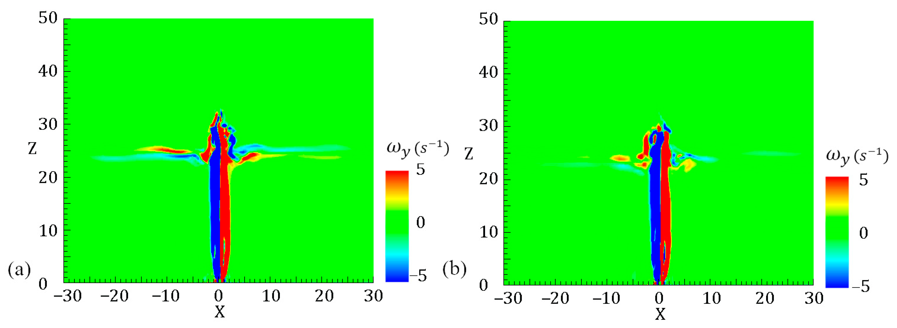
According to the flow field, it can be concluded that the jet can’t penetrate through the pycnocline completely in the range of 1.11 < Frp < 4.77. One part penetrates through the pycnocline, and falls back to the pycnocline again. The other part is blocked by the pycnocline. As a result, vortices with opposite directions are formed in pair on both sides of the pycnocline.
4.
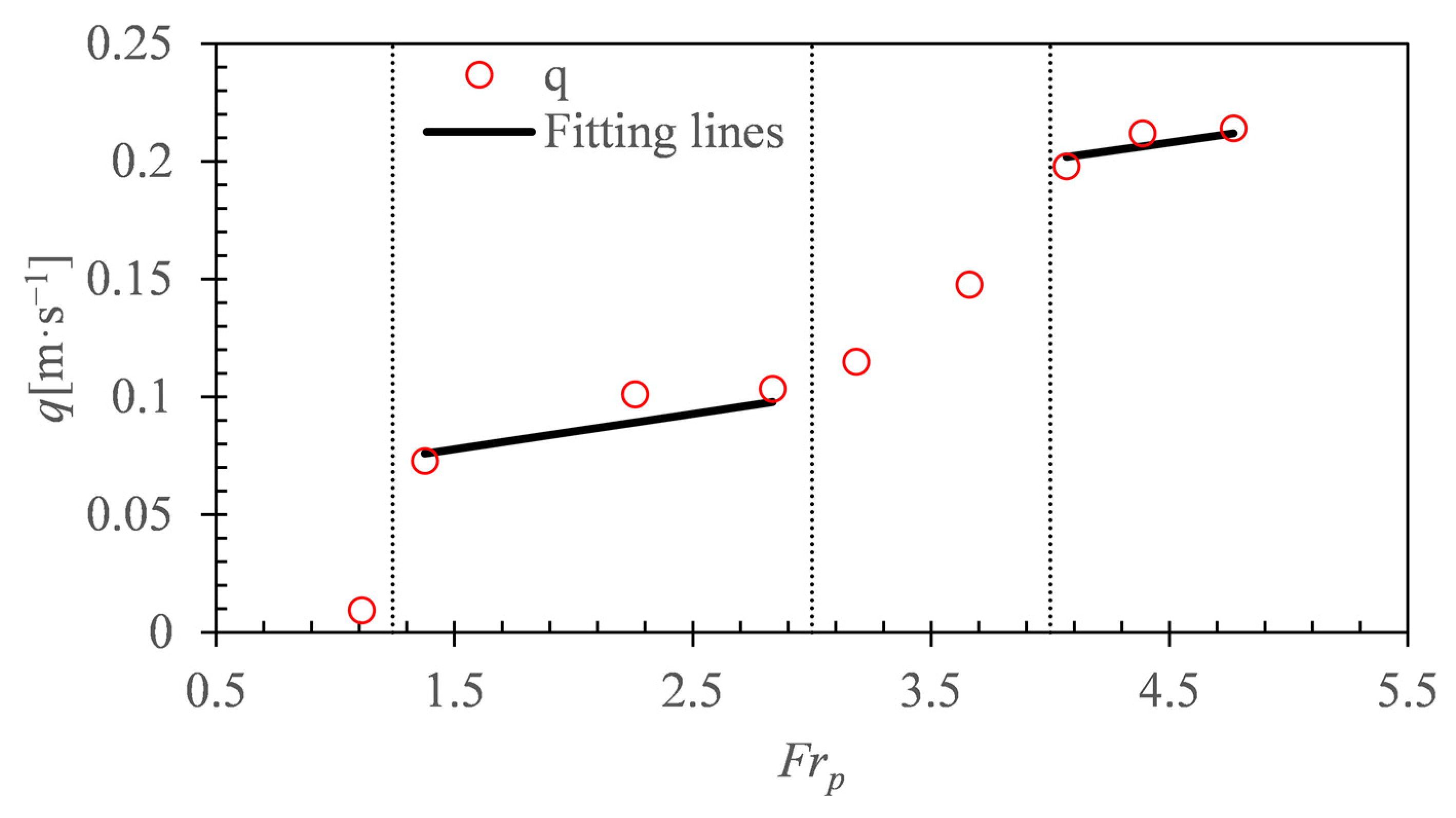
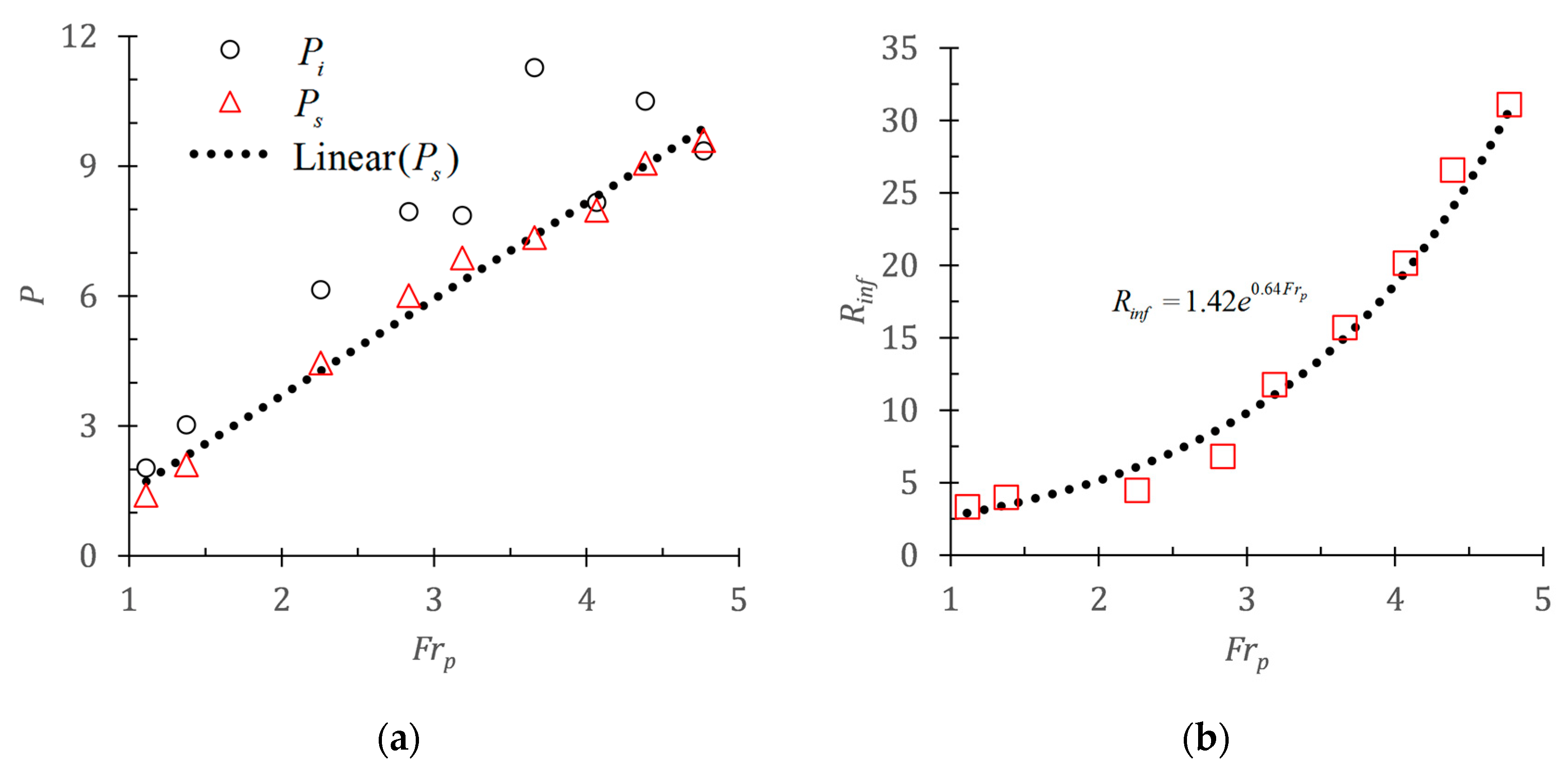
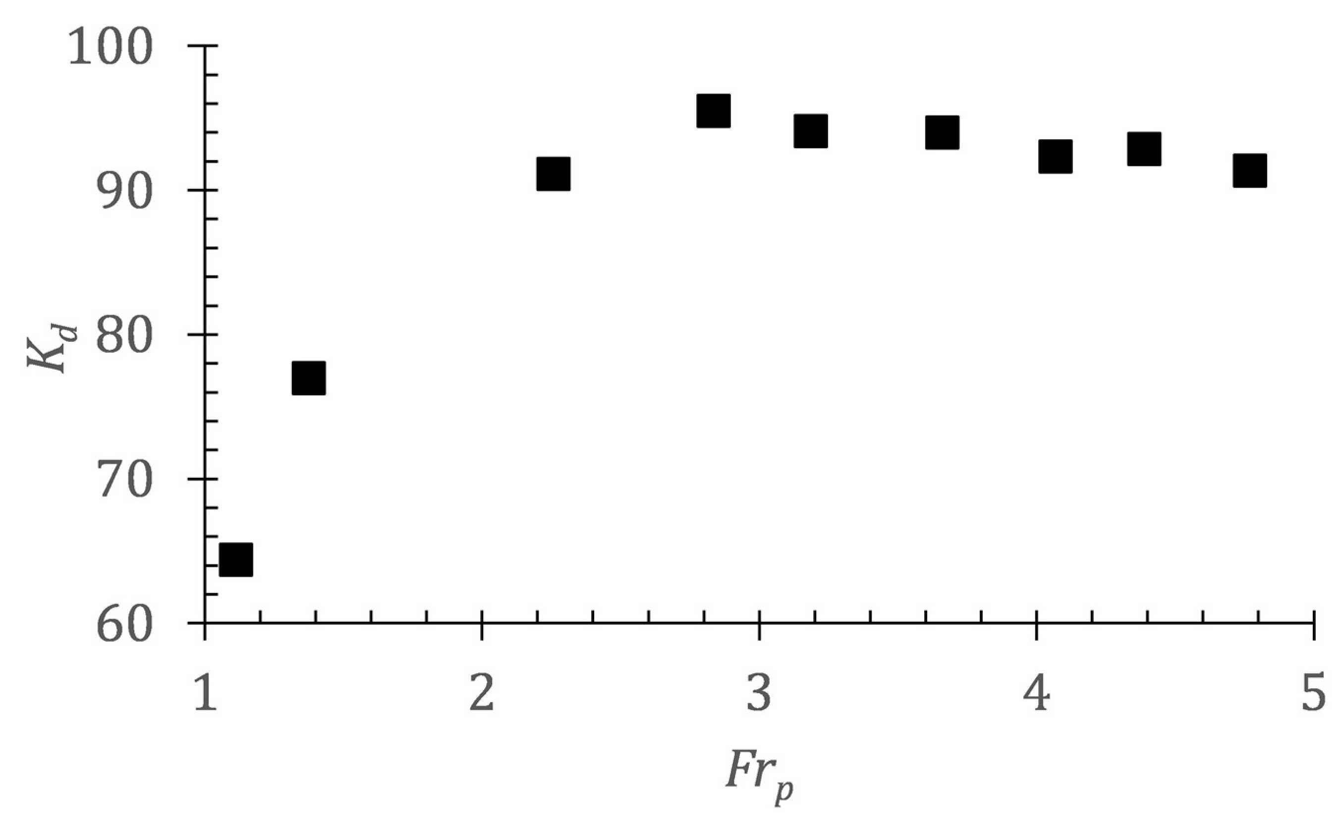
Frp = 3 is a threshold value of the interaction between jets and the pycnocline. When Frp > 3, the interaction becomes intensely. Hence, the jet affects a wider range under the influence of the strong turbulence, and the momentum of the jet is dissipated more efficiently, with a greater destratification effect of jets. In addition, the fitting formula of the radial momentum flux dissipation rate is established through dimensionless analysis.
5.
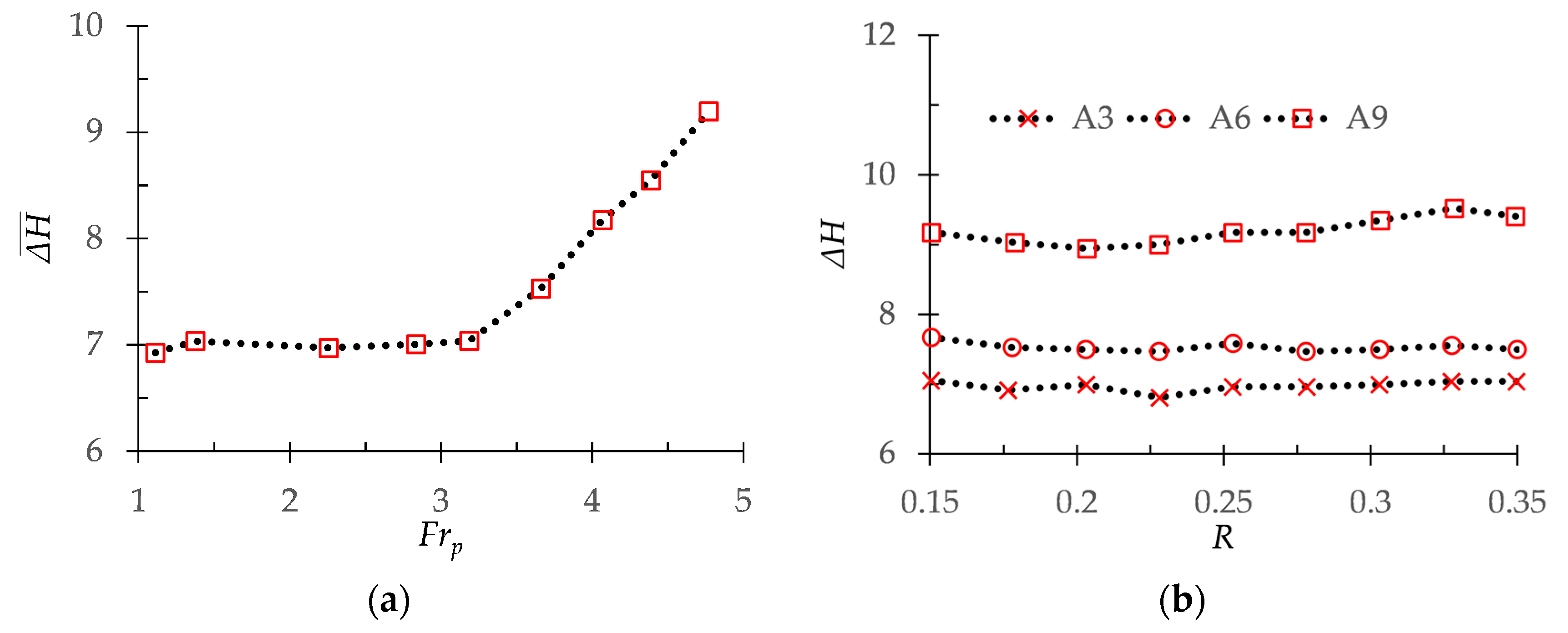
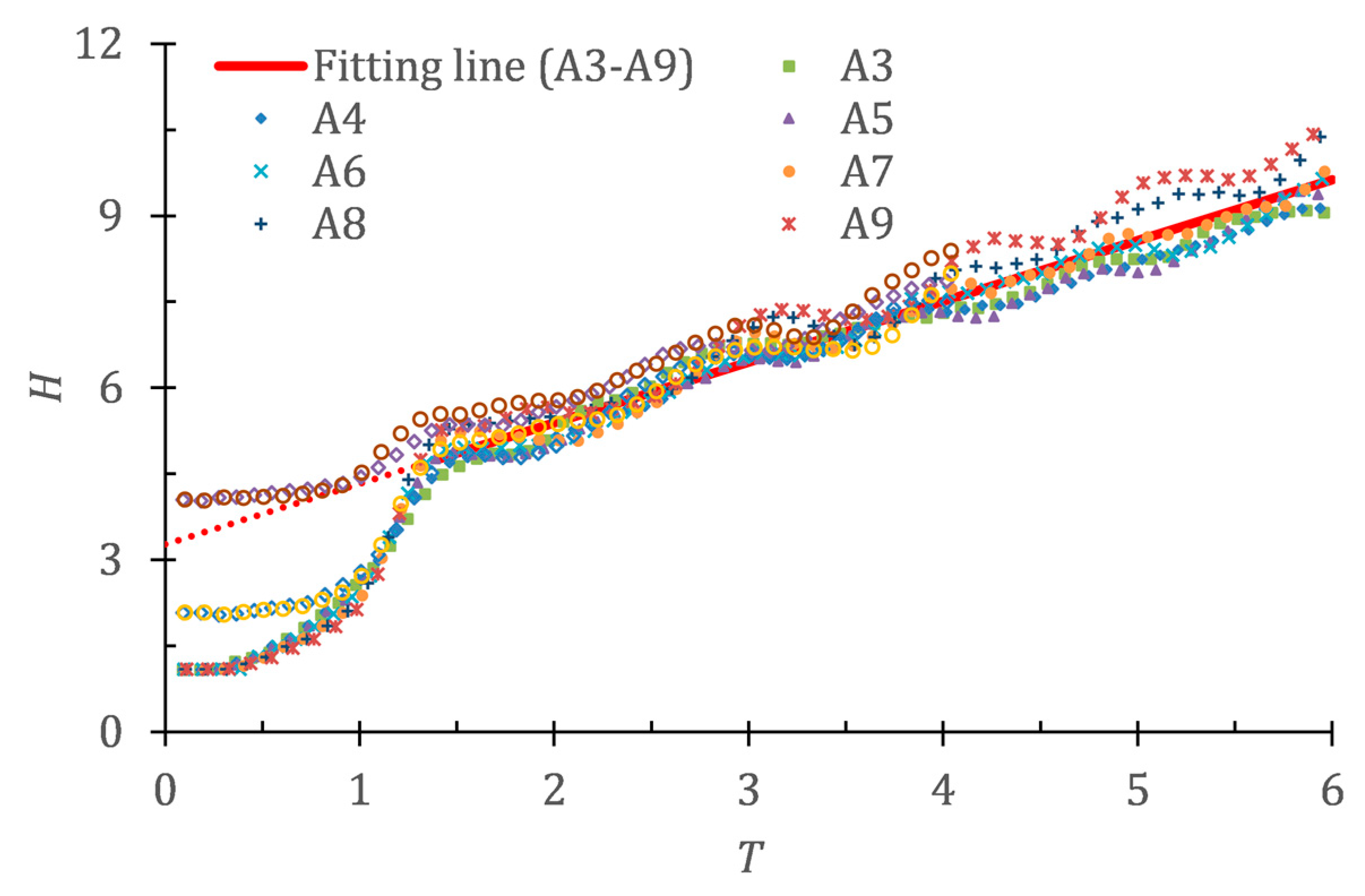
It is found that the destratification of the jet is mainly affected by the velocity of the internal waves produced by the jet. Regardless of the value of initial pycnocline thickness or Frp, the pycnocline thickness reaches the critical value at T = 1.4 with the influence of the first internal wave. When T > 1.4, the increasing rate apparently slows down and the pycnocline thickness increases linearly in all cases due to the vorticity in the pycnocline becomes small obviously after the thickness of the pycnocline reaches the critical value.
Additionally, re-suspension and entrainment of particles can be caused by jets, which is a common feature and is a complex problem in stratified environments. The study in this paper would give a potential factor of re-suspension and entrainment of particles caused by jets.

Author Contributions

Supervision, L.-l.W.; Writing—original draft, X.H.; Writing—review & editing, J.X. All authors have read and agreed to the published version of the manuscript.

Funding

This research was funded by National Key R&D Program of China (2017YFC0405605); National Natural Science Foundation of China (51879086); The 111 Project (B17015).

Conflicts of Interest

The authors declare no conflict of interest.

References

  1. Jirka, G.; Lee, J. Waste disposal in the ocean. In Water Quality and Its Control; Hino, M., Ed.; Balkema: Rotterdam, The Netherlands, 1994; Volume 5, pp. 193–242. [Google Scholar]
  2. Camilli, R.; Reddy, C.M.; Yoerger, D.R. Tracking hydrocarbon plume transport and biodegradation at deepwater horizon. Science 2010, 330, 201–204. [Google Scholar] [CrossRef]
  3. Ahmad, N.; Suzuki, T. Study of dilution, height, and lateral spread of vertical dense jets in marine shallow water. Water Sci. Technol. 2016, 73, 2986–2997. [Google Scholar] [CrossRef] [PubMed]
  4. Zordan, J.; Juez, C.; Schleiss, A.J.; Franca, M.J. Entrainment, transport and deposition of sediment by saline gravity currents. Adv. Water Resour. 2018, 115, 17–32. [Google Scholar] [CrossRef]
  5. Schleiss, A.J.; Franca, M.J.; Juez, C.; Cesare, G.D. Reservoir sedimentation. J. Hydraul. Res. 2016, 1–20. [Google Scholar] [CrossRef]
  6. Li, Y.; Huang, T.L.; Tan, X.L.; Zhou, Z.Z.; Ma, W.X. Destratification and oxygenation efficiency of a water-lifting aerator system in a deep reservoir: Implications for optimal operation. J. Environ. Sci. 2018, 73, 13–23. [Google Scholar] [CrossRef] [PubMed]
  7. Stephens, R.; Jörg, I. Reservoir destratification via mechanical mixers. J. Hydraul. Eng. 1993, 119, 438–457. [Google Scholar] [CrossRef]
  8. Fast, A.W. Effects of artificial destratification on primary production and Zoobenthos of El Capitan Reservoir California. Water Resour. Res. 1973, 9, 607–623. [Google Scholar] [CrossRef]
  9. Steinberg, C. Effects of artificial destratification on the phytoplankton populations in a small lake. Freshw. Biol. 1983, 5, 855–864. [Google Scholar] [CrossRef]
  10. Hamilton, D.P.; Chan, T.; Robb, M.S.; Robb, M.S.; Pattiaratchi, C.B.; Herzfeld, M. The hydrology of the upper Swan River Estuary with focus on an artificial destratification trial. Hydrol. Process. 2001, 15, 2465–2480. [Google Scholar] [CrossRef]
  11. Schladow, S.G. Lake destratification by bubble-plume systems: Design methodology. J. Hydraul. Eng. 1993, 119, 350–368. [Google Scholar] [CrossRef]
  12. Hill, D.F.; Vergara, A.M.; Parra, E.J. Destratification by mechanical mixers: Mixing efficiency and flow scaling. J. Hydraul. Eng. 2008, 134, 1772–1777. [Google Scholar] [CrossRef] [Green Version]
  13. Camassa, R.; Lin, Z.; Mclaughlin, R.M.; Mertens, K.; Tzou, C.; Walsh, J.; White, B. Optimal mixing of buoyant jets and plumes in stratified fluids: Theory and experiments. J. Fluid Mech. 2016, 790, 71–103. [Google Scholar] [CrossRef] [Green Version]
  14. Turner, J.S. Jets and plumes with negative or reversing buoyancy. J. Fluid Mech. 1966, 26, 779–792. [Google Scholar] [CrossRef]
  15. Burridge, H.C.; Hunt, G.R. The rise heights of low- and high-Froude-number turbulent axisymmetric fountains. J. Fluid Mech. 2012, 691, 392–416. [Google Scholar] [CrossRef]
  16. Burridge, H.C.; Hunt, G.R. The rhythm of fountains: The length and time scales of rise height fluctuations at low and high Froude numbers. J. Fluid Mech. 2013, 728, 91–119. [Google Scholar] [CrossRef]
  17. Ezhova, E.V.; Cenedese, C.; Brandt, L. Interaction between a vertical turbulent jet and a thermocline. J. Phys. Oceanogr. 2016, 46, 3415–3437. [Google Scholar] [CrossRef]
  18. Druzhinin, O.A.; Troitskaya, Y.I. Internal wave generation by a fountain in a stratified fluid. Fluid Dyn. 2010, 45, 474–484. [Google Scholar] [CrossRef]
  19. Ezhova, E.V.; Sergeev, D.A.; Soustova, I.A. On the structure of internal waves excited by buoyant plumes in stratified fluid. Bull. Russ. Acad. Sci. Phys. 2008, 72, 1701–1704. [Google Scholar] [CrossRef]
  20. Ezhova, E.V.; Sergeev, D.A.; Kandaurov, A.A. Nonsteady dynamics of turbulent axisymmetric jets in stratified fluid: Part 1. Experimental study. Izv. Atmos. Ocean. Phys. 2012, 48, 409–417. [Google Scholar] [CrossRef]
  21. Ezhova, E.V.; Troitskaya, Y.I. Nonstationary dynamics of turbulent axisymmetric jets in a stratified fluid: Part 2. Mechanism of excitation of axisymmetric oscillations in a submerged jet. Izv. Atmos. Ocean. Phys. 2012, 48, 528–537. [Google Scholar] [CrossRef]
  22. Cotel, A.J.; Gjestvang, J.A.; Ramkhelawan, N.N. Laboratory experiments of a jet impinging on a stratified interface. Exp. Fluids 1997, 23, 155–160. [Google Scholar] [CrossRef]
  23. Mcdougall Trevor, J. Bubble plumes in stratified environments. J. Fluid Mech. 1978, 85, 655–672. [Google Scholar] [CrossRef]
  24. Kim, S.H.; Kim, J.Y.; Park, H. Effects of bubble size and diffusing area on destratification efficiency in bubble plumes of two-layer stratification. J. Hydraul. Eng. 2010, 136, 106–115. [Google Scholar] [CrossRef] [Green Version]
  25. Neto, I.E.L.; Cardoso, S.S.S.; Woods, A.W. On mixing a density interface by a bubble plume. J. Fluid Mech. 2016, 802, R3. [Google Scholar] [CrossRef]
  26. Chen, Y.P.; Li, C.W.; Zhang, C.K. Numerical study of a round buoyant jet under the effect of JONSWAP random waves. China Ocean. Eng. 2012, 26, 235–250. [Google Scholar] [CrossRef]
  27. Ansong, J.K.; Kyba, P.J.; Sutherland, B.R. Fountains impinging on a density interface. J. Fluid Mech. 2008, 595, 115–139. [Google Scholar] [CrossRef] [Green Version]
  28. Zhu, H.; Wang, L.L.; Tang, H.W. Large-eddy simulation of suspended sediment transport in turbulent channel flow. J. Hydrodyn. 2013, 1, 48–55. [Google Scholar] [CrossRef]
  29. Lin, P.; Chi-Wai, L. A σ-coordinate three dimensional numerical model for surface wave propagation. Int. J. Numer. Methods Fluids 2002, 38, 1045–1068. [Google Scholar] [CrossRef]
  30. Park, J.C.; Kim, M.H.; Miyata, H. Fully non-linear free-surface simulations by a 3D viscous numerical wave tank. Int. J. Numer. Methods Fluids 2015, 29, 685–703. [Google Scholar] [CrossRef]
  31. Menow, S.; Rizk, M. Large-eddy simulations of forced three-dimensional impinging jets. Int. J. Numer. Methods Fluids 1996, 7, 275–289. [Google Scholar] [CrossRef]
  32. Zhou, X.; Luo, K.H.; Williams, J.J.R. Large-eddy simulation of a turbulent forced plume. Eur. J. Mech. B/Fluids 2001, 20, 233–254. [Google Scholar] [CrossRef]
  33. Jun, L.; Hong-Wu, T.; Ling-Ling, W. A novel dynamic coherent eddy model and its application to LES of a turbulent jet with free surface. Sci. China Phys. Mech. Astron. 2010, 53, 1671–1680. [Google Scholar]
  34. Xu, Z.; Chen, Y.; Zhang, C. Experimental study on the turbulent jet in regular and random waves. Adv. Water Sci. 2013, 24, 715–721. (In Chinese) [Google Scholar]
  35. Liu, C.Q.; Wang, Y.Q.; Yang, Y.; Duan, Z.W. New omega vortex identification method. Sci. China Phys. Mech. Astron. 2016, 59, 684711. [Google Scholar] [CrossRef]
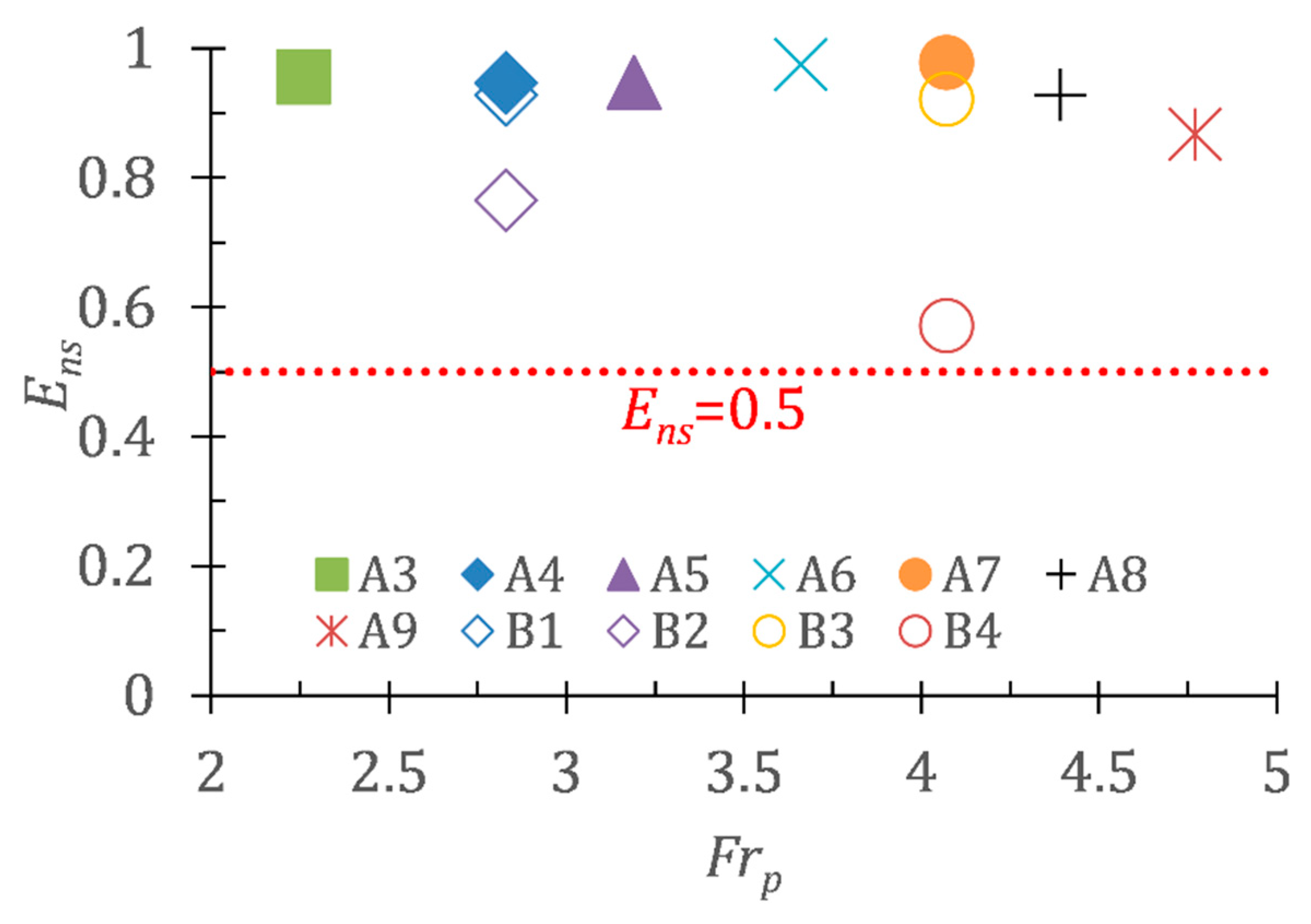
  36. Lin, F.; Chen, X.; Yao, H. Evaluating the use of Nash-Sutcliffe efficiency coefficient in goodness-of-fit measures for daily runoff simulation with SWAT. J. Hydrol. Eng. 2017, 22, 1–9. [Google Scholar] [CrossRef]
Figure 1. Schematic diagram of the jet interact with pycnocline.
Water 12 02085 g001
Figure 2. Schematic diagram of the turbulent jet in a stratified fluid.
Water 12 02085 g002
Figure 3. Diagram of 3D non-uniform cells.
Water 12 02085 g003
Figure 4. The correlation between u and v at the plane of Z = 20.
Water 12 02085 g004
Figure 5. The mean vertical velocity (a,b) and concentration (c,d) profiles of jets at Z = 20 in Case A0. The results of (a,c) are simulated by the azimuthal forcing method, and the results of (b,d) are simulated by the trigonometric function disturbance (TFD) method.
Water 12 02085 g005
Figure 6. Mesh refinement study. (a) Vertical velocity decay of the jet axis in Case A0. (b) Vertical velocity profiles of jets at the pycnocline in Case A9.
Water 12 02085 g006
Figure 7. The courant (CFL) number varying with Z at the jet axis. (a) Instantaneous CFL. (b) Mean CFL.
Water 12 02085 g007
Figure 8. Comparison between numerical results and experimental results.
Water 12 02085 g008
Figure 9. Gaussian and simulated velocity profile of the jet on the horizontal plane.
Water 12 02085 g009
Figure 10. Gaussian and simulated concentration profile of the jet on the horizontal plane.
Water 12 02085 g010
Figure 11. Comparison of present large eddy simulation (LES) data with vertical velocity profile of jet at the pycnocline by Ezhova and Troitskaya.
Water 12 02085 g011
Figure 12. Instantaneous density contours at the plane of Y = 0 during the jet impinging on the pycnocline in case A3. (af) corresponding to T = 0.24~0.67.
Water 12 02085 g012
Figure 13. Schematic of the initial penetration height (left) and the stable penetration height (right).
Water 12 02085 g013
Figure 14. Instantaneous density contours at planes of Y = 0 (left) and Z = 25 (right) when T = 0.6. And (a,b) are the case A1; (c,d) are the case A3; (e,f) are the case A9.
Water 12 02085 g014
Figure 15. The relationship between turbulent kinetic energy and Frp.
Water 12 02085 g015
Figure 16. Instantaneous coherent structures of Case A6 at T = 0.58. (a) Streamline around the jet at the plane of Y = 0. (b) Isosurface of Ω = 0.55.
Water 12 02085 g016
Figure 17. (a) Mean thicknesses of the pycnocline after the jet interaction with the pycnocline for 60 s. (b) The thickness distributions of the pycnocline in the range of 15 < R < 35 in cases A3, A6, and A9.
Water 12 02085 g017
Figure 18. Dimensionless changes in the penetration height (a) and the horizontal influence radius (b) vary with Frp.
Water 12 02085 g018
Figure 19. Momentum flux dissipation rate of jets vs Frp.
Water 12 02085 g019
Figure 20. Dissipation of radial momentum flux of cases A1~A9.
Water 12 02085 g020
Figure 21. Dimensionless change in the thickness of the pycnocline varies with time for Cases A3~A9 (Frp = 2.26~4.77) and B1~B2 (Frp = 2.83) and B3~B4 (Frp = 4.07). The red solid line is the fitting line when T > 1.4.
Water 12 02085 g021
Figure 22. Nash–Sutcliffe efficiency coefficients of Cases A3~A9 (Frp = 2.26~4.77) and B1~B2 (Frp = 2.83) and B3~B4 (Frp = 4.07).
Water 12 02085 g022
Figure 23. Instantaneous contour of ωy at T = 1.1 (a) and T = 2.2 (b) of case A6.
Water 12 02085 g023
Table 1. Dimensionless nozzle size of previous researches compared with the size in this study.
Dimensionless Nozzle SizeStratified/UnstratifiedExperimental/NumericalFr0Re0Reference
0.025StratifiedNumerical7~22-Ezhova [17]
0.01StratifiedExperimental-896~1066Ansong [27]
0.017StratifiedExperimental-6900 and 12,400Cotel [22]
0.0083StratifiedExperimental9–18.82979~5960Ahmad [3]
0.0041~0.0088UnstratifiedExperimental0.3~40563~4037Burridge [16]
0.033StratifiedNumerical1~9-Druzhinin [18]
0.0088StratifiedNumerical8.36~27.891760~8800This study
Table 2. The parameters of different cases. The Froude number Frp and Reynolds number Rep are defined at the entrance of the pycnocline, corresponding to the initial Froude number Fr0 and Reynolds number Re0. The details of values used in Table 2 can be found in Section 2.4.
Casesw0Fr0Re0FrpRepHρu (kg/m3)ρd (kg/m3)
A00.8824.537744---998998
A10.25.5817601.111393.071.09981033
A20.38.3626401.371723.631.09981033
A30.411.1635202.262828.661.09981033
A4 *0.513.9444002.833553.581.09981033
A50.616.7452803.193993.691.09981033
A60.719.5261603.664588.041.09981033
A7 *0.822.3170404.075099.321.09981033
A80.925.1079204.395500.411.09981033
A91.027.8988004.775979.111.09981033
B10.513.9444002.833553.582.09981033
B20.513.9444002.833553.584.09981033
B30.822.3170404.075099.322.09981033
B40.822.3170404.075099.324.09981033
* The parameters in B1~B2 and B3~B4 are refer to those in A4 and A7 respectively.

