A New Set of Local Indices Applied to a Water Network through Demand and Pressure Driven Analysis (DDA and PDA)

Abstract

In the analysis of drinking Water Distribution Networks (WDNs), performance indices are widely used tools for obtaining synthetic information about the WDN operating regime (pressures and flows). This paper presents applications of a series of local surplus indices that act in a new mathematical framework. This framework allows reworking many well-known performance and energetic indices and simultaneously allowing analysis of specific aspects of the WDN. The analyses are carried out using different resolutive hydraulic approaches: the Demand-Driven Analysis (DDA) and the Pressure-Driven Analysis (PDA), typical of software such as EPANET and WaterNetGen. The authors analyse the hypotheses necessary for the application of these models, and how these influence the results of both the hydraulic modeling and the resilience indices assessment. In particular, two resilience indices are reformulated through the new local surplus indices and all of them are then simulated in different conditions for a water network known in literature as the Kang and Lansey WDN. The solving model assumption effects are deepen, reporting graphical and numerical results for different consumption scenarios and the different hydraulic approaches used.

1. Introduction

Residential and productive agglomerations are characterized by an intricate network of underground services. These services are necessary to transfer resources such as gas, water, and electricity. The drinking Water Distribution Networks (WDNs) are complex systems, composed of kilometers of underground pipes and a large number of artifacts. Performance evaluation tools result useful in the study and modeling of those infrastructures.

Modeling Water Distribution Networks (WDNs) is often a difficult challenge and it is necessary to gather a vast amount of data that allows to characterize geometrically and hydraulically the constituent elements of the network (pipes, valves, pumps, etc.) and the network topology. Moreover, also the water demand of the served utilities have to be accurately defined together with the peak requests (see Section 3.2). The difficulty in modeling WDNs, in addition to the hydraulic and topological ones outlined above, is also since they are rarely equipped with Advanced Metering Infrastructures (AMI) and it is usually very hard to know the real conditions of degradation of the various elements making up a Water Distribution Network (WDN), often very old.

In the scientific literature, many models assess the operating regime of WDNs. Resolutive model types and complexity vary depending on the quantity and quality of the available data. New lines of research are also emerging in relation to current aspects and problems such as climate changes (see, for example [1,2]), system vulnerability and different kinds of risks (see [3,4,5,6,7] and, in particular, [8] concerning possible terrorist attacks), the use of rainwater and the reuse of wastewater (see [9,10]), etc., in a framework of sustainable management of water resources increasingly urgent (see also [11,12,13,14,15]).

In the performance assessment and analysis of WDNs, different tools and methodologies are usually employed (see for example [16,17,18,19,20,21,22,23,24,25,26,27,28,29,30,31,32]), among which there are several performance indices of various nature. These indices allow to evaluate, locally or globally, some characteristics of the WDN like energy surplus, entropy, energy efficiency, resilience, etc. (see [15,33,34,35,36,37,38,39,40]).

In the present paper, the authors want to assess the effectiveness of a new set of local indices proposed firstly in [41] and subsequently used in [42,43,44] for the network and performance analysis of a water supply system. Local indices allow to reformulate, in a new way, many more complex global indices and, in particular, this work uses and investigates the new formulations obtained for the resilience indices introduced by Todini in [45] and Di Nardo and others in [34,35,46,47,48,49,50]. Since the local surplus indices refer to the design conditions, attention has been paid to the effects of the assumptions needed for the application of the various resolutive approaches. To show the potentialities of the new indices through a local approach, in opposition to the use of global indices, the local surplus indices have been assessed for different consumption scenarios as well.

Finally, different hydraulic solvers that exploit two distinct calculation approaches are also used: Demand Driven Analysis and Pressure Driven Analysis, or in brief, DDA and PDA, respectively.

Among the various benefits that can derive from a local indices approach such as that obtained by exploiting the local surplus indices, the authors want to signal the possibility of their easy implementation in different hydraulic simulation software (see for example [42] in about WaterNetGen implementation), in decision support system interfaces or, hopefully in the future, in real-time monitoring devices, with immediate benefits for water managers. In large part, the easy applicability is determined by the versatility and manageability of the linear algebra and vector analysis tools (see in particular [41]) which naturally operate on these indices. Many other theoretical and practical uses are still being studied and developed; for instance, the local surplus indices together with subsequent steps of the mathematical framework introduced in [41], allow to deepen some problems such as the invariance of many global hydraulic parameters and to propose new ones that are not affected by these problems (see, for example, [51] for a first initiative in this direction).

2. Materials and Methods

To conduct the research presented in this paper, two sets of tools that interact with each other are employed, one of a more theoretical nature and the other computational: the next two subsections are respectively devoted to their brief description and analysis. In Section 2.1, a new set of local energetic indices, originally presented in [41], are introduced under various forms and with the help of the basic tools of a mathematical fr amework specifically designed for them. In Section 2.2, on the other hand, the hydraulic software models and settings, that allow explicit computations with local indices on the WDN, are examined. In particular, Section 2.2.1 and Section 2.2.2 are devoted to DDA and PDA methodologies, respectively. Finally, Section 2.2.3 enlightens the simulation settings and the needed hypotheses to their actual application, with a close comparison of the differences between the two approaches.

2.1. Local Performance Indices

Let $\mathcal{N}$ be a WDN having n junction nodes, m linking pipes between nodes and r reservoirs/tanks. For each $k=1,\dots ,r$, we denote by $Q_k$ and $H_k$ the discharge and the head, respectively, of the k-th reservoir, hence the total available hydraulic power $P_{tot}$ fed into the water network $\mathcal{N}$ can be calculated as follows (see for example [34,35,41,43,44,45,47,48,49,50])

$$P_{tot}=\gamma \sum _{k=1}^r{Q}_k{H}_k,$$

(1)

where $\gamma =\rho g$ denotes, as usual, the specific weight of water and $\rho$ stands for its density. The previous equation holds in the absence of pumps, otherwise, the pumps power has to be added to Equation (1) and the formulas and the whole discussion of the next pages accordingly modified, see for instance [45] (Equation (4)). For each $i=1,\dots ,n$ let $q_i$ and $h_i$ be the outgoing flow and the head, respectively, at the node i, thus $p_i=\gamma q_i{h}_i$ is the delivered power at that node. The piezometric head $h_i$ is decomposed as $h_i=z_i+{𝒽}_i$ where $z_i$ is the geodetic elevation and ${𝒽}_i$ the pressure head of the node i, respectively. As usual, we also adopt the star notation to indicate the corresponding project conditions or minimum requests: more precisely, $q_i^{*}$, ${𝒽}_i^{*}$, $h_i^{*}$ and $p_i^{*}=\gamma q_i^{*}{h}_i^{*}$ denote the project discharge (water supply), pressure head, piezometric head and power relative to the node i, respectively (see, for example, [45] or [34,49,50] and the references therein). Thus, the total minimum power $P_{Emin}$ that must be delivered to the nodes of the whole network to satisfy the project constraints, is given by

$$P_{Emin}=\gamma \sum _{i=1}^n{q}_i^{*}{h}_i^{*},$$

(2)

and

$$P_{Dmax}=P_{tot}-P_{Emin}=\gamma \left(\sum _{k=1}^r{Q}_k{H}_k-\sum _{i=1}^n{q}_i^{*}{h}_i^{*}\right)$$

(3)

represents the maximum dissipable power, i.e., the highest power that can be dispersed without compromising the satisfaction of the project constraints in any node. Similarly, if $P_E=\gamma {\sum }_{i=1}^n{q}_i{h}_i$ is the total amount of delivered power to the output nodes $i=1,\dots ,n$, then the energetic balance of the network $\mathcal{N}$ is given by

$$P_{tot}=P_D+P_E,$$

where $P_D$ is the total dissipated power or internal power of $\mathcal{N}$, i.e.,

$$P_D=\sum _{u=1}^m{\tilde{q}}_u\Delta h_u,$$

where ${\tilde{q}}_u$ is the flow and $\Delta h_u$ the head loss along the u-th pipe, $u=1,2,\dots ,m$.

The ratio between the internal power and the maximum dissipable one gives rise to an important and widespread index in many fields of engineering that wants to evaluate the ability of the system to adapt and cope with sudden or unplanned events (for example, breakdowns, failures, changes due to previously unforeseeable circumstances, etc.). More precisely, the resilience index $I_R$ of the water network $\mathcal{N}$, as defined and used by Di Nardo et al. in [34,35,46,47,48,49,50], is given by

$$I_R=1-\frac{P_D}{P_{Dmax}}=\frac{{\displaystyle \sum _{i=1}^n}\left(q_i{h}_i-q_i^{*}{h}_i^{*}\right)}{{\displaystyle \sum _{k=1}^r}{Q}_k{H}_k-{\displaystyle \sum _{i=1}^n}{q}_i^{*}{h}_i^{*}}.$$

(4)

The index $I_R$ has a small discrepancy respect to the original one, $I_r$, introduced by Todini in [45]: if $P_D^{*}$ denotes the following power difference

$$P_D^{*}=P_{tot}-\gamma \sum _{i=1}^n{q}_i^{*}{h}_i,$$

then $I_r$ is defined as

$$I_r=1-\frac{{\displaystyle P_D^{*}}}{{\displaystyle P_{Dmax}}}=\frac{{\displaystyle \sum _{i=1}^n}{q}_i^{*}\left(h_i-h_i^{*}\right)}{{\displaystyle \sum _{k=1}^r}{Q}_k{H}_k-{\displaystyle \sum _{i=1}^n}{q}_i^{*}{h}_i^{*}}$$

(5)

(for an extensive review of these and many other resilience indices, the reader can see [39]).

Assuming that there are no flow and head deficiencies in the network $\mathcal{N}$, i.e., $q_i\ge q_i^{*}\ge 0$ and $h_i\ge h_i^{*}\ge 0$ for all $i=1,\dots ,n$, then, between the two resilience indices defined in (4) and (5), the following relation holds

$$0\le I_r\le I_R\le 1$$

(6)

But in many real cases the empirical (or simulated) data sets do not distinguish between the nodal supply $q_i$ and demand $q_i^{*}\ge 0$ (see the next subsection for further insights about the solving software hypothesis), that is, it is often employed the following assumption

$$q_i=q_i^{*}\mathrm{for}\mathrm{all}i=1,2,\dots ,n.$$

(7)

The first consequence obtained by assuming condition (7) concerns the coincidence of the two resilience indices $I_R$ and $I_r$, as the reader can easily verify from (4) and (5).

Using the above defined fundamental quantities, in [41] the authors propose a set of local surplus indices as elementary bricks to build and re-write many energetic indices both of local and global nature for a WDN. Together with the avant-garde of a mathematical framework specifically designed for this purpose and which allows to adequately handle these local indices, the authors also want to highlight in [41] the importance of pursuing a local-global analysis for a WDN and not just a study limited to the evaluation of indices of global type.

In particular, in [41] the following indices are defined (see also [42,43] and [44])

$$\begin{array}{cccc}{q}_i^s\hfill & :=\hfill & \frac{q_i-q_i^{*}}{q_i^{*}}\hfill & \mathit{Local}\mathit{discharge}\mathit{surplus}\mathit{index},\hfill \\ {𝒽}_i^s\hfill & :=\hfill & \frac{{𝒽}_i-{𝒽}_i^{*}}{{𝒽}_i^{*}}\hfill & \mathit{Local}\mathit{pressure}\mathit{head}\mathit{surplus}\mathit{index},\hfill \\ h_i^s\hfill & :=\hfill & \frac{h_i-h_i^{*}}{h_i^{*}}\hfill & \mathit{Local}\mathit{piezometric}\mathit{head}\mathit{surplus}\mathit{index},\hfill \\ p_i^s\hfill & :=\hfill & \frac{p_i-p_i^{*}}{p_i^{*}}=\frac{q_i{h}_i-q_i^{*}{h}_i^{*}}{q_i^{*}{h}_i^{*}}\hfill & \mathit{Local}\mathit{power}\mathit{surplus}\mathit{index},\hfill \end{array}$$

(8)

where $i=1,2,\dots ,n$. Moreover, they are collected in vectors giving rise to the following local surplus vectors

$$\begin{array}{cccc}\overrightarrow{q^s}\hfill & :=\hfill & \left(q_1^s,q_2^s,\dots ,q_n^s\right)\hfill & \mathit{Local}\mathit{discharge}\mathit{surplus}\mathit{vector},\hfill \\ \overrightarrow{{𝒽}^s}\hfill & :=\hfill & \left({𝒽}_1^s,{𝒽}_2^s,\dots ,{𝒽}_n^s\right)\hfill & \mathit{Local}\mathit{pressure}\mathit{head}\mathit{surplus}\mathit{vector},\hfill \\ \overrightarrow{h^s}\hfill & :=\hfill & \left(h_1^s,h_2^s,\dots ,h_n^s\right)\hfill & \mathit{Local}\mathit{piezometric}\mathit{head}\mathit{surplus}\mathit{vector},\hfill \\ \overrightarrow{p^s}\hfill & :=\hfill & \left(p_1^s,p_2^s,\dots ,p_n^s\right)\hfill & \mathit{Local}\mathit{power}\mathit{surplus}\mathit{vector},\hfill \end{array}$$

(9)

and finally, by convenience, it is useful to organize all data in vector format:

$$\begin{array}{cc}\overrightarrow{Q}:=(Q_1,Q_2,\dots ,Q_r),\hfill & \overrightarrow{H}:=(H_1,H_2,\dots ,H_r),\hfill \\ \overrightarrow{q}:=(q_1,q_2,\dots ,q_n),\hfill & \overrightarrow{q^{*}}:=(q_1^{*},q_2^{*},\dots ,q_n^{*}),\hfill \\ \overrightarrow{𝒽}:=({𝒽}_1,{𝒽}_2,\dots ,{𝒽}_n),\hfill & \overrightarrow{{𝒽}^{*}}:=({𝒽}_1^{*},{𝒽}_2^{*},\dots ,{𝒽}_n^{*}),\hfill \\ \overrightarrow{h}:=(h_1,h_2,\dots ,h_n),\hfill & \overrightarrow{h^{*}}:=(h_1^{*},h_2^{*},\dots ,h_n^{*}),\hfill \\ \overrightarrow{p}:=(p_1,p_2,\dots ,p_n),\hfill & \overrightarrow{p^{*}}:=(p_1^{*},p_2^{*},\dots ,p_n^{*}),\hfill \end{array}$$

and

$$\overrightarrow{z}:=(z_1,z_2,\dots ,z_n).$$

It is moreover easy to find relations between the local indices (8) as, for example, the following

$$p_i^s=q_i^s{h}_i^s+q_i^s+h_i^s,$$

(10)

which holds for all $i=1,2,\dots ,n$ (cf. (11)), or similar others.

A last piece of notation regards some well-known tools of linear algebra. If $\overrightarrow{x}=(x_1,x_2,\dots ,x_n)$ and $\overrightarrow{y}=(y_1,y_2,\dots ,y_n)$ are two vectors of the real n-space ${\mathbb{R}}^n$, the standard scalar product between them is denoted by $\overrightarrow{x}$·$\overrightarrow{y}$, instead the Hadamard product is denoted by $\overrightarrow{x}$∘$\overrightarrow{y}$ and is defined as their component-wise product (see [41] or [52]), i.e.,

$$\overrightarrow{x}\circ \overrightarrow{y}:=(x_1·y_1,x_2·y_2,\dots ,x_n·y_n).$$

For instance, using the Hadamard product, the set of n relations of the type (10) between local indices can be concisely expressed in the form

$$\overrightarrow{p^s}=\overrightarrow{q^s}\circ \overrightarrow{h^s}+\overrightarrow{q^s}+\overrightarrow{h^s}$$

(11)

as relation between local vectors.

Example 1.

The resilience indices $I_R$ and $I_r$ are very similar to one another and it is therefore not immediate, looking at (4) and (5), to give a hydraulic interpretation of the differences between them. Using local vectors instead, it is clear that $I_R$ is to the local surplus power vector $\overrightarrow{p^s}$ as $I_r$ is to the local surplus piezometric head vector $\overrightarrow{h^s}$ (see (14)). In fact, by adopting the aforementioned mathematical framework, described in more detail in [41], $I_R$ and $I_r$ can be written respectively as

$$I_R=\frac{\overrightarrow{p^s}·\overrightarrow{p^{*}}}{\gamma \left(\overrightarrow{Q}·\overrightarrow{H}-\overrightarrow{q^{*}}·\overrightarrow{h^{*}}\right)}$$

(12)

and

$$I_r=\frac{\overrightarrow{h^s}·\overrightarrow{p^{*}}}{\gamma \left(\overrightarrow{Q}·\overrightarrow{H}-\overrightarrow{q^{*}}·\overrightarrow{h^{*}}\right)},$$

(13)

or equivalently as

$$I_R=\overrightarrow{p^s}·\frac{\overrightarrow{q^{*}}\circ \overrightarrow{h^{*}}}{\overrightarrow{Q}·\overrightarrow{H}-\overrightarrow{q^{*}}·\overrightarrow{h^{*}}}\mathit{and}{I}_r=\overrightarrow{h^s}·\frac{\overrightarrow{q^{*}}\circ \overrightarrow{h^{*}}}{\overrightarrow{Q}·\overrightarrow{H}-\overrightarrow{q^{*}}·\overrightarrow{h^{*}}}.$$

(14)

Through (12), $I_R$ can be read as the mean value of the entries of the minimal power request vector weighted by the local power surplus vector $\overrightarrow{p^s}$ and normalized by the factor $\gamma \left(\overrightarrow{Q}·\overrightarrow{H}-\overrightarrow{q^{*}}·\overrightarrow{h^{*}}\right)$, instead for $I_r$, the role of the weight vector is played by $\overrightarrow{h^s}$ (see (13)).

Other possible applications and advantages of using local indices and local vectors inside a more organized and rich mathematical framework as exposed in [41], can be also found in [42,43,44,51], as well as in [41]. In conclusion of the present subsection, it is important to emphasize how the matrix and vector forms and the linear algebra tools traced above, allow easy and useful implementations in many engineering software and numerical computing systems like, for instance, MATLAB (whose name itself stands for MATrix Laboratory, see also [25]).

2.2. Hydraulic Software Solvers

A WDN having a fixed and well-known structural conformation and geometry is considered so that all the structural data of the network can be modeled and calibrated (for example, the elevations represented by the vector $\overrightarrow{z}$, the lengths, the diameters, the pipes roughness coefficients, etc.).

As already mentioned in the Introduction, from a computational point of view, two are the major resolutive approaches most followed in the current literature: demand driven and pressure driven modeling, previously written through the acronyms DDA and PDA, respectively. In DDA the nodal discharges $q_i$ are assumed to be known as input data, hence there is no distinction between $q_i$ and $q_i^{*}$, and (7) holds. If the sum of the flows entering the water network is equal to the sum of the flows supplied from it (i.e., ${\sum }_{k=1}^r{Q}_k={\sum }_{i=1}^n{q}_i$), and the heads $H_k,k=1,\dots ,r$, are sufficiently high, then the solver computes the nodal heads and the flows through all the pipes of the network (see Section 2.2.1 for more technical details). On the other hand, if the heads $H_k,k=1,\dots ,r$, are not sufficient to guarantee the required nodal discharges, then the software stops the simulation without obtaining a full solution for the network (or continue the simulation obtaining inconclusive results, as negative pressures).

If the heads of the reservoirs (and the network structure) allow a complete satisfaction of the supply requests in the nodes, then there are no significant differences using DDA or PDA. The results instead change when a pressure driven approach is used in the case of a WDN that registers pressure deficits (local or more extensive).

In this work, for both PDA and DDA, WaterNetGen (vers. 1.0.0.942) is used. WaternNetGen is a well-known software for hydraulic simulation, an EPANET extension developed by J. Muranho et al. (see [53,54]). WaterNetGen incorporates all the capabilities of EPANET, providing a user-friendly graphical interface. Both WaterNetGen and EPANET allow to perform DDA and PDA using [55] (Equation (1)).

In a pressure driven model, the discharge at the node i is equal to the request if the local pressure head is greater or equal to a certain threshold value ${𝒽}_i^{\mathrm{req}}$, called service pressure threshold or, for short, service pressure, which represents the minimal pressure needed to completely satisfy the supply; in symbols, $q_i=q_i^{*}$ if ${𝒽}_i\ge {𝒽}_i^{\mathrm{req}}$. In case of a local deficit of pressure, contrary to the DDA approach, the PDA based model carries out the simulation representing a rather realistic scenario in all the points of the network. In particular, t the PDA model contemplates two subcases: if the pressure ${𝒽}_i$, at the node i, is less than a second threshold value ${𝒽}_i^{min}\left(<{𝒽}_i^{\mathrm{req}}\right)$, which represents the minimal pressure under which there is no supply at all, then $q_i=0$, instead, if ${𝒽}_i$ is between ${𝒽}_i^{min}$ and ${𝒽}_i^{\mathrm{req}}$, then the discharge $q_i$ depends on ${𝒽}_i$ through an exponential-type formula (see (19) and Section 2.2.2 for more details). However, the downside to report for the PDA model is that, as a counterpart to a greater adherence to reality, it is sometimes quite more expensive in computational terms and data needs.

2.2.1. Demand Driven Analysis

This subsection is devoted to a more in-depth examination of how the DDA model works. For every $i=1,\dots ,n$ let $n\left(i\right)$ be the number of junction nodes linked to the node i (hence ${\sum }_{i=1}^{n}n\left(i\right)=2m$, where m is the total number of pipes linking two nodes as defined at the beginning of Section 2.1) and assume the data $Q_k,H_k$ for $k=1,\dots ,r$ and $q_i$ for $i=1,\dots ,n$ to be given. To find a solution for the network, the software solves the following system of $n\left(i\right)+1$ equations for every node $i=1,2,\dots ,n$

$$\{\begin{array}{cc}{q}_i-{\displaystyle \sum _{j=1}^{n\left(i\right)}}{Q}_{ij}=0,\hfill & \hfill \mathrm{(15)}\\ h_i-h_j=h_{ij}=R·Q_{ij}^e+m_l·Q_{ij}^2\mathrm{for}\mathrm{all}j=1,2,\dots ,n\left(i\right)& \hfill \mathrm{(16)}\end{array}$$

where $Q_{ij}$ and $h_{ij}$ are, respectively, the flow and the headloss along the pipe connecting the node i and j (for all $j=1,2,\dots ,n\left(i\right)$), R is a friction coefficient, e the flow exponent in the energy equation (called also headloss formula) and $m_l$ is a minor loss coefficient (see, e.g., [56] and the references therein for more explanations). Moreover, for short, $h_j=h_j^i$ denotes in (16) the piezometric head at the j-th node connected to the base node i, where j runs, of course, between 1 and $n\left(i\right)$. Equation (15) is often referred as the continuity flow equation at the node i and Equation (16) as the equation describing the energy law in the linking pipe between two nodes.

As regards the consequences on local indices of using successfully a DDA approach on a given WDN, the first thing is to note that the equalities expressed in (7) are then all valid by hypothesis, i.e., $q_i=q_i^{*}$ for every $i=1,2,\dots ,n$. Hence this implies the nullity of all the local discharge surplus indices

$$q_i^s=\frac{q_i}{q_i^{*}}-1=1-1=0\mathrm{for}\mathrm{every}i=1,2,\dots ,n,$$

(17)

and the equality between the local power surplus index and the local piezometric head surplus one, that is

$$p_i^s=\frac{p_i}{p_i^{*}}-1=\frac{q_i{h}_i}{q_i^{*}{h}_i^{*}}-1=\frac{h_i}{h_i^{*}}-1=h_i^s\mathrm{for}\mathrm{all}i=1,2,\dots ,n.$$

(18)

Another consequence of the successful use of a DDA approach on a WDN would be the coincidence of the resilience indices $I_R$ and $I_r$: it follows, in fact, by using (18) in (14), or (7) in (4) and (5). Note finally that a successful use of a DDA approach, on the other hand, does not predict anything on the sign of the last three local indices in (8), and the minimal project requests on the pressure heads ${𝒽}_i^{*}$ do not affect the computing procedure and the results obtained by the software, but only the local indices ${𝒽}_i^s$ and $h_i^s$.

In case the software finds a low-pressure regime occurring in some nodes or fails instead to find a full solution, this means that some nodal pressure is not sufficient to ensure the full supply in that node (i.e., the hypothesis $q_i=q_i^{*}$ does not hold everywhere) and it is necessary to study the WDN by using another approach, for instance, a PDA model.

2.2.2. Pressure Driven Analysis

PDA software usually adds to each system of $n\left(i\right)+1$ Equations (15) and (16), based on the node i, the following further equation that expresses the water discharge $q_i$ as a function of the pressure head ${𝒽}_i$ (see [53,54,55])

$$q_i\left({𝒽}_i\right)=q_i^{*}·\left\{\begin{array}{cc}1\hfill & \mathrm{if}{𝒽}_i\ge {𝒽}_i^{\mathrm{req}},\hfill \\ {\displaystyle {\left(\frac{{𝒽}_i-{𝒽}_i^{min}}{{𝒽}_i^{\mathrm{req}}-{𝒽}_i^{min}}\right)}^{\alpha }}\hfill & \mathrm{if}{𝒽}_i^{min}<{𝒽}_i<{𝒽}_i^{\mathrm{req}},\hfill \\ 0\hfill & \mathrm{if}{𝒽}_i\le {𝒽}_i^{min},\hfill \end{array}\right.$$

(19)

where ${𝒽}_i^{\mathrm{req}}$ and ${𝒽}_i^{min}$ are the two threshold values defined before Section 2.2.1, i.e., ${𝒽}_i^{\mathrm{req}}$ is the minimal pressure that allows a complete satisfaction of the demand $q_i^{*}$, and ${𝒽}_i^{min}$ is the minimal pressure above which the supply starts and below which there is no supply at all. Finally, $\alpha \in {\mathbb{R}}^{+}$ is the exponent of the pressure-discharge relationship.

To examine the repercussions of using a PDA approach in resolving a WDN on the local indices at the node i, three cases must be distinguished according to whether ${𝒽}_i\ge {𝒽}_i^{\mathrm{req}}$, ${𝒽}_i^{min}<{𝒽}_i<{𝒽}_i^{\mathrm{req}}$ or ${𝒽}_i\le {𝒽}_i^{min}$. If ${𝒽}_i\ge {𝒽}_i^{\mathrm{req}}$, there are no substantial differences for the node i using a PDA or a DDA approach and, in particular, (7), (17) and (18) continue to hold as shown in Section 2.2.1.

If ${𝒽}_i^{min}<{𝒽}_i<{𝒽}_i^{\mathrm{req}}$ then (see (19))

$$0<q_i=q_i^{*}·{\left(\frac{{𝒽}_i-{𝒽}_i^{min}}{{𝒽}_i^{\mathrm{req}}-{𝒽}_i^{min}}\right)}^{\alpha }<q_i^{*}$$

(20)

and, consequently, the local discharge surplus index $q_i^s$ is negative, more precisely

$$q_i^s=\frac{q_i}{q_i^{*}}-1={\left(\frac{{𝒽}_i-{𝒽}_i^{min}}{{𝒽}_i^{\mathrm{req}}-{𝒽}_i^{min}}\right)}^{\alpha }-1<0.$$

Moreover, the local power surplus index $p_i^s$ can be easily written as follows

$$p_i^s=\frac{p_i}{p_i^{*}}-1=\frac{q_i{h}_i}{q_i^{*}{h}_i^{*}}-1={\left(\frac{{𝒽}_i-{𝒽}_i^{min}}{{𝒽}_i^{\mathrm{req}}-{𝒽}_i^{min}}\right)}^{\alpha }·\frac{h_i}{h_i^{*}}-1,$$

but it is not possible to make predictions on its sign. Lastly note that if, in addition, the threshold value ${𝒽}_i^{\mathrm{req}}$ is assumed equal to the minimal project request ${𝒽}_i^{*}$ and ${𝒽}_i^{min}$ is zero, then

$$\frac{q_i}{q_i^{*}}={\left(\frac{{𝒽}_i}{{𝒽}_i^{*}}\right)}^{\alpha }$$

and the formulas for $q_i,q_i^s$ and $p_i^s$ above would be simplified considerably.

To consider the third case, if ${𝒽}_i\le {𝒽}_i^{min}$, then it is immediate that $q_i=0$ and $q_i^s=p_i^s=-1$.

2.2.3. Simulation Settings and Hypotheses

It is convenient to clearly define the hypotheses necessary to estimate the resilience indices and the local surplus ones, in particular in the light of the so-called peak coefficient.

The simulations carried out for both the DDA and PDA approach are in steady flow. The defined peak coefficient $P_c$ multiplies the base demand in each junction node of the WDN and is applied in both cases. In PDA simulations, in accordance with Section 2.2.2 and with Equation (19), ${𝒽}_i^{\mathrm{req}}$ and ${𝒽}_i^{min}$ must be defined for each node. Although ${𝒽}_i^{\mathrm{req}}$ and ${𝒽}_i^{*}$ are different things, for computational purposes it has been assumed that the reference pressure coincides with the design required one. On the other hand, the minimum pressure threshold ${𝒽}_i^{min}$ is set to 0 meters, both to simplify computations and since there are no particularly high elevation differences in the place of the network in question. The pressure values ${𝒽}_i^{min}$, ${𝒽}_i^{\mathrm{req}}$ and ${𝒽}_i^{*}$, instead, are not directly involved in the simulation settings for DDA analysis (recall, in particular, (15) and (16)).

In Section 3, the numerical computation of the resilience index $I_r$ (as well as $I_R$), is affected by the chosen setting. For DDAs, this index, which coincides with $I_R$ (see Section 2.2.1), has the total available energy (1) where

$$\sum _{k=1}^r{Q}_k=\sum _{i=1}^n{q}_i$$

(21)

(considering a WDN with no leaks, or the leaks assigned as nodal demand) and $q_i=q_i^{*}$ for all $i=1,2,\dots ,n$ (see Section 2.2.1 and, in particular, its references to (7)). On the other hand, the $I_r$ index in PDAs uses the same total available power (1) with the assumption (21) of no water leaks, but allowing $q_i\le q_i^{*}$ for all $i=1,2,\dots ,n$ (see Section 2.2.2 and recall, in particular, (19) and (20)).

Analogous observations can be made using the total power (1) in the computation of the resilience index $I_R$.

3. Results and Discussion

This section provides some experimental results concerning the topics exposed in Section 2 and, in particular, the local indices defined in (8). The subject of the calculations is the network described in Section 3.1. Section 3.2 focuses on peak coefficient settings for the simulation, while Section 3.3 shows the resulting indices for different simulation scenarios.

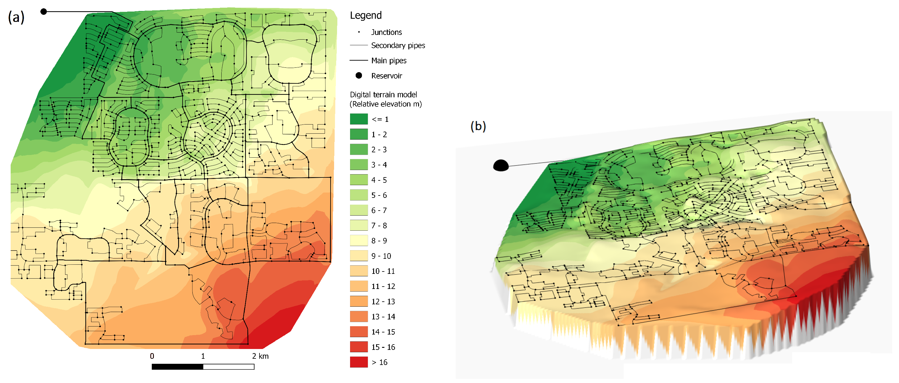
3.1. Test Network and Requested Condition

To better evaluate the usefulness of the local surplus indices, them are used, along with the resilience indices in the performance assessment of a medium-sized network. The considered network is the one proposed by Kang and Lancey in [57].

This network consists of 935 nodes and 1274 pipes, which extend for $252\mathrm{km}$. For 623 of these nodes, there is a non-zero design discharge request, while for the remaining 312, $q_i^{*}=0$. Kang and Lancey in [57] give indications on the target pressure value (28 meters) and on the peak coefficient to be used to take into account the hourly fluctuations in the application (i.e., $P_c=1.75$). In particular, this means that the minimal design pressure request, unlike $q_i^{*}$, is the same for all the nodes of the WDN, i.e., ${𝒽}_i^{*}=28m$ for all $i=1,2,\dots ,935$.

The average consumption of the network is 177.21 l/s and the peak consumption ($P_c=1.75$) is 310.11 l/s. The whole network is supplied by a pumping station, modeled as a reservoir (infinite volume and fixed piezometric head). The network is characterized by a limited elevation variability. Figure 1 shows the relative elevation of the nodes relating to the lowest node of the network. The zero relative elevation node is located at 391.15 m above sea level. The higher areas are located in the peripheral zone, far from the reservoir, in the lower right corner. The maximum relative elevation is 16.46 m. The reservoir is located at 413.31 m above sea level (63.9 m of relative elevation).

Figure 2 shows the network operating regime for the conditions indicated by the authors in [57]. The simulation shows that for these settings the network has a good piezometric head regime. The whole WDN is above the requested pressure head of 28 m. The areas characterized lower pressures are the ones located at a higher elevation and far from the reservoir (down right corner).

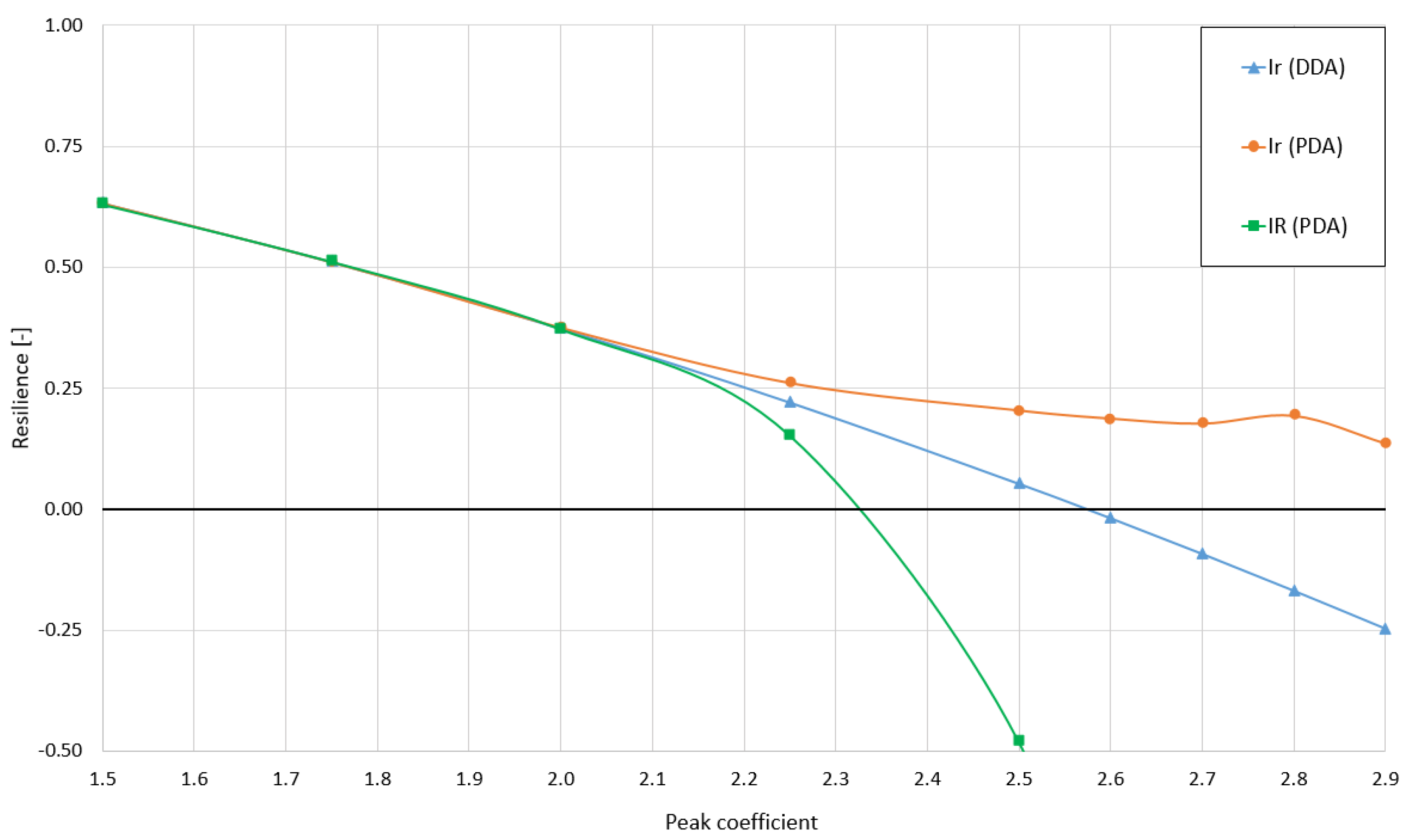
3.2. Peak Coefficients

The paper aims to assess the variability of local and resilience indices for different scenarios. The simulation involves the performance of different simulations (PDA and DDA) characterized by different peak coefficients. The demand for drinking water that the networks must satisfy is not a fixed value but varies at different time scales. The need for water has many seasonal components that vary on an annual, daily, and hourly scale. To simplify this variability, peak coefficients are used. A peak coefficient is a multiplicative coefficient that represents the ratio between the demand under conditions of peak consumption and the average ones. For the KL network, the authors in [57] indicate the average annual flow and a peak coefficient necessary to represent the hourly variation. Peak coefficients are usually also influenced by the type and size of population centers. Networks like the one presented in this paper are usually serving medium-sized cities. In the absence of data, the authors have assessed the population served, imposing an average value of water supply of 250 L per inhabitant per day (see, for example, [58]). The served population is assessed on about 60,000 inhabitants. In the simulation, the peak coefficient varies to model both the average consumption and excessive consumption scenarios. The network resilience is calculated accordingly to the peak factor variation. For cities with 60,000 inhabitants, the peak coefficients for periods of maximum yearly consumption can exceed 2 or 3 times the average value in particular conditions.

In this paper, simulations with a wide range of peak coefficients were performed to model different consumption scenarios. The chosen peak coefficients are 1.5, 1.75, 2, 2.25, 2.5, 2.6, 2.7, 2.8, and 2.9.

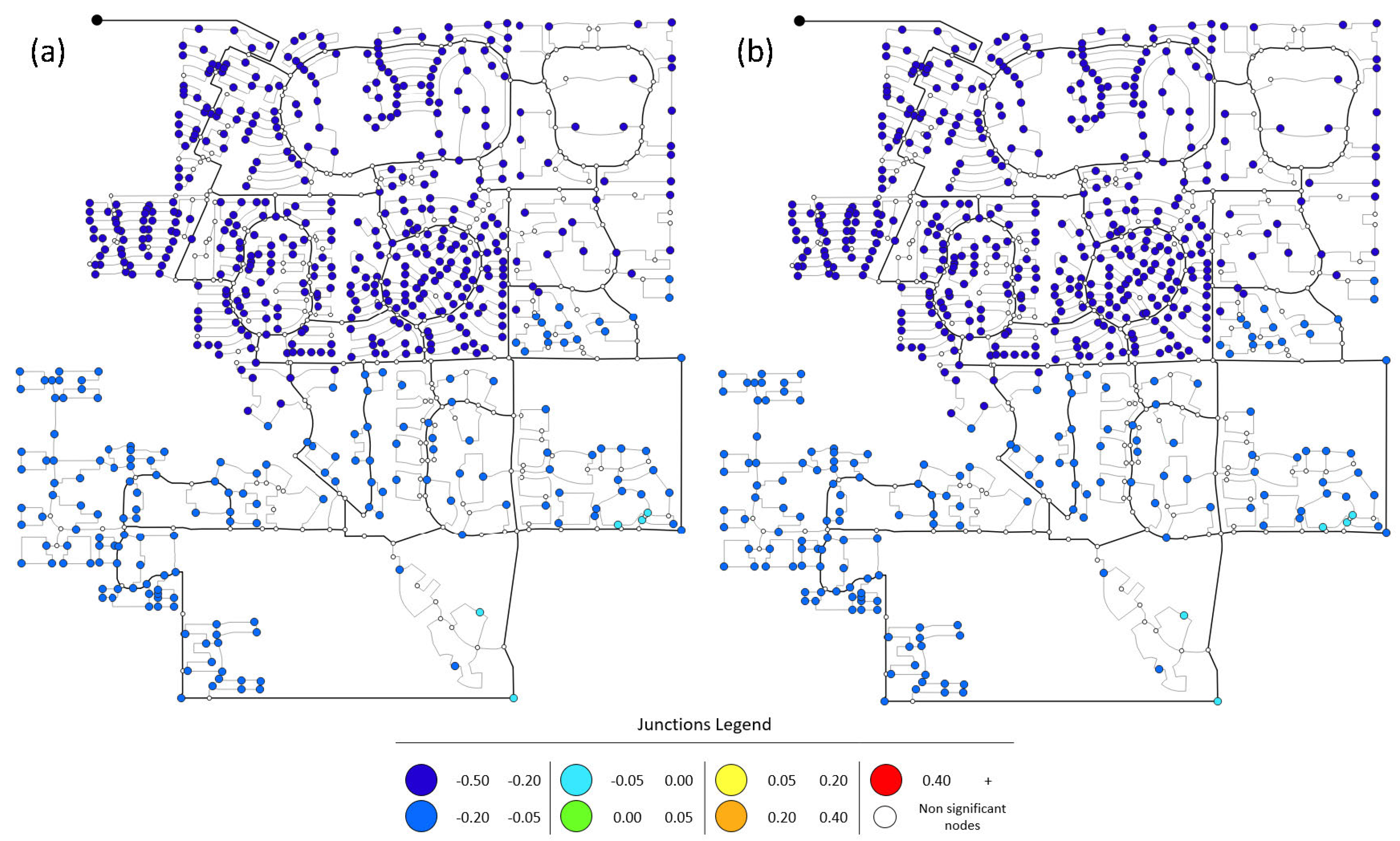
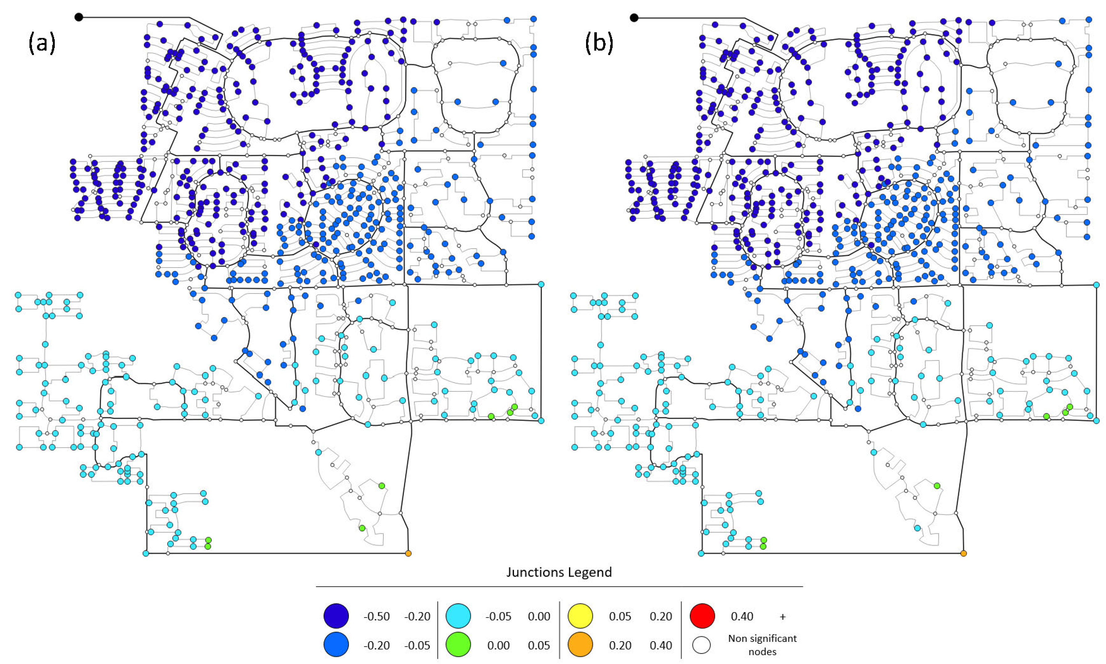
3.3. Simulation Results

The resilience indices, for each of the peak coefficients, are shown in

Table 1. Some values of the resilience indices $I_r$ and $I_R$ depending on the peak coefficient $P_c$. In the second column Todini’s index $I_r$ is computed by using the DDA approach, instead in the third by using a PDA approach. The fourth column gives the index $I_R$ obtained through a PDA approach.

${\mathit{P}}_{\mathit{c}}$	${\mathit{I}}_{\mathit{r}}$ by DDA	${\mathit{I}}_{\mathit{r}}$ by PDA	${\mathit{I}}_{\mathit{R}}$ by PDA
1.50	0.632	0.632	0.629
1.75	0.511	0.511	0.511
2.00	0.373	0.375	0.371
2.25	0.221	0.261	0.152
2.50	0.053	0.204	−0.482
2.60	−0.018	0.187	−1.134
2.70	−0.092	0.177	−2.842
2.80	−0.168	0.193	−17.969
2.90	−0.247	0.135	7.503

and Figure 3. It should be noted that, due to the assumptions made in (7), the indices, in absence of pressure deficit conditions, coincide (unless small approximations due to the software, as in the first row of Table 1 for the peak coefficient $P_c=1.5$). It is also immediate to note that for high peak coefficients, which can be found in particular conditions, the calculation of the network resilience provides no significant values (see Figure 3 or Table 1). In particular, $I_R$ with $P_c$ between 2.8 and 2.9, has a vertical asymptote, and a sign change. Todini’s index $I_r$ changes instead of sign.

The change of sign is bound to the achievement of a condition in which the minimum required energy for the network design conditions is greater than the available one:

$$P_{Emin}>P_{tot}\mathrm{and}{P}_{Dmax}<0$$

A similar result may be representative of two possible scenarios:

• The network is subjected to stress for which it is not designed for, and it works in conditions of excessive demand and, consequently, pressure deficit.
• The required conditions are too stringent and far from reality.

In the case in question, having no information regarding the indications given in [57] on the pressure limit and the peak coefficient, the achievement of this condition is due to an excessive synthetic increase in the request for the resource

$$P_{Dmax}>P_{tot}$$

Below are shown some graphical results obtained using the local surplus indices. These indices were calculated for 4 of the simulations shown in Table 1 (i.e., $P_c=1.75,2,2.25,2.5$). Since they are always null, the values of the local discharge surplus index $q_i^s$ are not shown for DDA simulations. Both the values of $h_i^s$ and $p_i^s$ are very flattened due to the elevation values $z_i$ contained within them, thus resulting in little significance as synthetic standalone indicators. The comparisons between the graphs containing the local pressure index ${𝒽}_i^s$, obtained by PDA and DDA simulations having the same $P_c$, and the graphs of the local discharge surplus index for the 4 chosen peak factors, are therefore reported.

Figure 4 and Figure 5a show the results obtained by the water simulation with a peak coefficient of 1.75. This peak coefficient, being not particularly high, does not determine deficit conditions and the consequent lack of water supply for junctions. As it can be seen from Figure 2, the pressure in the WDN remains above the requested value for all the junction nodes. The absence of pressure deficit conditions means that the local pressure head surplus index assumes only positive values. A good pressure regime implies the absence of a deficit in the water supply, therefore the local discharge surplus index is always null, see Figure 5a. It should be noted that, due to the assumptions made in (7), both the results of the simulations and the indices, in the absence of pressure deficit conditions, coincide.

The increase of the peak coefficient ($P_c=2$) leads to an overall reduction in the pressure of the network, caused by the higher circulating flows, necessary to satisfy a greater demand. Increased demand leads to conditions close to those requested, see Figure 5b and Figure 6. A single junction is characterized by deficit conditions. This junction is located in a particularly high area far from the reservoir (see Figure 1a). Since deficit conditions are limited to a single node, it is not possible to appreciate particular differences between the results of PDA and DDA simulations or resilience indices values (See Table 1).

Another increase in the peak coefficient ($P_c=2.25$), determines pressure deficit condition in the network which must satisfy a water demand of about 30% greater than the simulation with $P_c=1.75$. In that case, the central area of the network is characterized by a condition close to the required ones, while in the peripheral area, the pressure regime is not sufficient to guarantee a full supply, see Figure 7 and Figure 8a.

Since a good number of junctions nodes present deficit conditions, it is possible to notice differences between the results of the DDA and PDA simulations. The reduced amount of delivered water, modeled by PDA simulations, involves a reduction of the flows circulating in the network. This reduction leads to a decrease of the head losses alongside the pipes, therefore the results of PDA simulations are generally characterized by lower pressure deficits.

The last simulation uses a peak coefficient of 2.5. In this case, the peak coefficient imposes a consume about 40% higher than the simulation with $P_c=1.75$. The network reaches a condition very far from the requested one. Only the parts near the reservoir do not show a deficit (see Figure 8b and Figure 9). As the deficit conditions increase, the difference between the network operating regime, resulting from PDA and DDA simulations, increases.

There are no graphs characterized by peak coefficients greater than 2.5 because they represent situations very far from reality.

In the first column of

Table 2. The number of nodes in deficit or surplus pressure condition for each of the ranges used in Figure 4 and Figure 6. The second column, for example, reports the number of nodes in any range, with reference to Figure 4a (i.e., DDA approach with $P_c=1.75$).

${\mathbf{𝒽}}_{\mathit{i}}^{\mathit{s}}$ Range	1.75, DDA	1.75, PDA	2.00, DDA	2.00, PDA
$]-0.50;-0.20]$	0	0	0	0
$]-0.20;-0.05]$	0	0	1	1
$]-0.05;0]$	0	0	0	0
$]0;0.05]$	0	0	7	6
$]0.05;0.20]$	5	5	140	141
$]0.20;0.40]$	174	174	203	203
${𝒽}_i^s>0.40$	444	444	272	272
Not significant	312	312	312	312

, seven different ranges, correspondent to the colors used in Figure 4 and Figure 6, are listed. The first and second columns refer to Figure 4a,b, respectively, while the third and fourth columns refer to Figure 6a,b.

Table 3. The number of nodes subdivided by range of pressure deficit and surplus, as appear in Figure 7 and Figure 9, that is, $P_c$ equal to 2.25 or 2.5.

${\mathbf{𝒽}}_{\mathit{i}}^{\mathit{s}}$ Range	2.25, DDA	2.25, PDA	2.50, DDA	2.50, PDA
$]-0.50;-0.20]$	1	1	135	56
$]-0.20;-0.05]$	69	62	80	120
$]-0.05;0]$	67	63	75	26
$]0;0.05]$	28	32	56	78
$]0.05;0.20]$	148	140	129	159
$]0.20;0.40]$	202	201	81	113
${𝒽}_i^s>0.40$	108	124	67	71
Not significant	312	312	312	312

, similarly to Table 2, shows the number of nodes in pressure deficit or surplus for Figure 7 and Figure 9.

Table 4. The number of nodes for range of supply deficit as appear in Figure 5 and Figure 8. Obviously, it can be done only for the PDA approach. The last line reports, for completeness, the number of nodes without water demand, i.e., with $q_i^s=0$ and $q_i^{*}=0$ m${}^3$/h.

${\mathit{q}}_{\mathit{i}}^{\mathit{s}}$ Range	1.75	2.00	2.25	2.50
$]-0.20;-0.10]$	0	0	1	62
$]-0.10;-0.05]$	0	0	21	86
$]-0.05;-0.01]$	0	1	55	39
$]-0.01;-0.002]$	0	0	40	6
$]-0.002;0]$	623	622	506	430
Not significant	312	312	312	312

shows the number of water supply deficit nodes, divided in 5 classes, for PDA simulations with different peak coefficients (see Figure 5 and Figure 8).

4. Conclusions

This paper exploits the local surplus indices introduced firstly in [41] and successively used in [42,43,44,51], and also the mathematical framework started in [41] as well, which allows to employ the former in several ways and to derive from them other well-known indices and measures for a WDN such as, for example, the indices of resilience introduced by Todini and Di Nardo et al. (see [34,35,45,46,47,48,50], respectively). Both indices have therefore been reformulated in a new and compact way, through which it is easier to analyse the role of the individual components that come into play, to make comparisons between similar indices, and to identify possible recurrent hidden or deeper structures.

The potential of such an approach that exploits local surplus indices also as mathematical tools is not limited only to interpreting resilience indices in a new key, but the same can be done with many other global indices already known in literature, as shown in more detail in [41]. Hence the importance of investigating in depth the local indices on real WDNs, both as information carriers and as “building bricks” to obtain more.

The use of a complex WDN, such as the one proposed by Kang and Lansey in [57], has allowed the authors to expose hypotheses and limits of the solution approach most used in literature. Many performance indices refer to the design or “required” conditions. The definition of these conditions is a very delicate phase since it can compromise the significance of these indices.

The resilience indices were also employed to deepen the study on the definition of the required conditions. Many works do not specify the values or assumptions used to define these conditions. In this paper, both the local surplus indices and the resilience ones have been stressed through several different scenarios to deepen the correct definitions of the required conditions.

Two of the local surplus indices have also been used as graphical indicators of the network state. These indices provided immediate information on the deviations of the network nodes from the required conditions, showing the degree of satisfaction of the demand and the state of the network pressure regime. In particular, from the four local indices defined in (8), the first two were chosen, $q_i^s$ and ${𝒽}_i^s$, to represent graphically in Figure 2, Figure 3, Figure 4, Figure 5, Figure 6, Figure 7 and Figure 8 the nodal performances of the network and to allow easy comparisons between districts.

References

1. Cervarolo, G.; Mendicino, G.; Senatore, A. Re-modulating water allocation in a complex multi-reservoir system under current and climate change scenarios. Eur. Water 2012, 37, 47–57. [Google Scholar]
2. Maiolo, M.; Mendicino, G.; Pantusa, D.; Senatore, A. Optimization of Drinking Water Distribution Systems in Relation to the Effects of Climate Change. Water 2017, 9, 803. [Google Scholar] [CrossRef]
3. Davis, M.J.; Janke, R. Patterns in potential impacts associated with contamination events in water distribution systems. J. Water Resour. Plan. Manag. 2011, 137, 1–9. [Google Scholar] [CrossRef]
4. Gheisi, A.; Forsyth, M.; Naser, G. Water distribution systems reliability: A review of research literature. J. Water Resour. Plann. Manag. 2016, 142, 04016047. [Google Scholar] [CrossRef]
5. Loucks, D.P. Quantifying System Sustainability Using Multiple Risk Criteria: Risk, Reliability, Uncertainty, and Robustness of Water Resources Systems; Cambridge University Press: Cambridge, UK, 2002. [Google Scholar]
6. Maiolo, M.; Pantusa, D. A methodological proposal for the evaluation of potable water use risk. Water Pract. Technol. 2015, 10, 152–163. [Google Scholar] [CrossRef]
7. Maiolo, M.; Pantusa, D.; Chiaravalloti, F.; Carini, M.; Capano, G.; Procopio, A. A New Vulnerability Measure for Water Distribution Network. Water 2019, 10, 1005. [Google Scholar] [CrossRef] [Green Version]
8. Maiolo, M.; Pantusa, D. Infrastructure vulnerability index of drinking water supply systems to possible terrorist attacks. Cogent Eng. 2018, 5, 1456710. [Google Scholar] [CrossRef]
9. Maiolo, M.; Pantusa, D. Combined reuse of wastewater and desalination for the management of water systems in conditions of scarcity. Water Ecol. 2017, 72, 116–126. [Google Scholar]
10. Maiolo, M.; Pantusa, D. A proposal for multiple reuse of urban wastewater. J. Water Reuse Desalin. 2018, 8, 468–478. [Google Scholar] [CrossRef] [Green Version]
11. Böhringer, C.; Jochem, P.E. Measuring the immeasurable—A survey of sustainability indices. Ecol. Econ. 2007, 63, 1–8. [Google Scholar] [CrossRef] [Green Version]
12. Maiolo, M.; Carini, M.; Capano, G.; Piro, P. Synthetic sustainability index (SSI) based on life cycle assessment approach of low impact development in the Mediterranean area. Cogent Eng. 2017, 4, 1410272. [Google Scholar] [CrossRef]
13. Maiolo, M.; Martirano, G.; Morrone, P.; Pantusa, D. Assessment criteria for a sustainable management of water resources. Water Pract. Technol. 2006, 1. [Google Scholar] [CrossRef]
14. Maiolo, M.; Pantusa, D. An optimization procedure for the sustainable management of water resources. Water Sci. Technol. Water Supply 2016, 16, 61–69. [Google Scholar] [CrossRef]
15. Maiolo, M.; Pantusa, D. Sustainable Water Management Index, SWaM_Index. Cogent Eng. 2019, 6, 1603817. [Google Scholar] [CrossRef]
16. Agathokleous, A.; Christodoulou, C.; Christodoulou, S.E. Topological Robustness and Vulnerability Assessment of Water Distribution Networks. Water Resour. Manag. 2017, 31, 4007–4021. [Google Scholar] [CrossRef]
17. Bi, W.; Dandy, G.C.; Maier, H.R. Improved genetic algorithm optimization of water distribution system design by incorporating domain knowledge. Environ. Model. Softw. 2015, 69, 370–381. [Google Scholar] [CrossRef]
18. Bragalli, C.; Fortini, M.; Todini, E. Data assimilation in water distribution systems. Procedia Eng. 2017, 186, 506–513. [Google Scholar] [CrossRef]
19. Candelieri, A.; Giordani, I.; Archetti, F. Supporting Resilience Management of Water Distribution Networks through Network Analysis and Hydraulic Simulation. In Proceedings of the 21st International Conference on Control Systems and Computer Science, Bucharest, Romania, 29–31 May 2017. [Google Scholar]
20. Candelieri, A.; Soldi, D.; Archetti, F. Network analysis for resilience evaluation in water distribution networks. Environ. Eng. Manag. J. 2015, 14, 1261–1270. [Google Scholar] [CrossRef]
21. Dai, J.; Wu, S.; Han, G.; Weinberg, J.; Xie, X.; Wu, X.; Song, X.; Jia, B.; Xue, W.; Yang, Q. Water-energy nexus: A review of methods and tools for macro-assessment. Appl. Energy 2018, 210, 393–408. [Google Scholar] [CrossRef]
22. D’Ambrosio, C.; Lodi, A.; Wiese, S.; Bragalli, C. Mathematical programming techniques in water network optimization. Eur. J. Oper. Res. 2015, 243, 774–788. [Google Scholar] [CrossRef]
23. Di Nardo, A.; Di Natale, M.; Giudicianni, C.; Greco, R.; Santonastaso, G.F. Complex network and fractal theory for the assessment of water distribution network resilience to pipe failures. Water Sci. Technol. Water Supply 2017, 18, 767–777. [Google Scholar] [CrossRef]
24. Di Nardo, A.; Di Natale, M.; Santonastaso, G.; Venticinque, S. An automated tool for smart water network partitioning. Water Resour. Manag. 2013, 27, 4493–4508. [Google Scholar] [CrossRef]
25. Eliades, D.G.; Kiriakou, M.; Vrachimis, S.; Polycarpou, M.M. EPANET-MATLAB Toolkit: An Open-Source Software for interfacing EPANET with MATLAB. In Proceedings of the 14th International Conference on Computing and Control for the Water Industry (CCWI), Amsterdam, The Netherlands, 7–9 November 2016. [Google Scholar]
26. Ferrari, G.; Savíc, D.; Becciu, G. Graph-theoretic approach and sound engineering principles for design of district metered areas. J. Water Resour. Plann. Manag. 2014, 140, 04014036. [Google Scholar] [CrossRef] [Green Version]
27. Hamiche, A.M.; Stambouli, A.B.; Flazi, S. A review of the water-energy nexus. Renew. Sustain. Energy Rev. 2016, 65, 04016047. [Google Scholar] [CrossRef]
28. Herrera, M.; Abraham, E.; Stoianov, I. A Graph-Theoretic Framework for Assessing the Resilience of Sectorised Water Distribution Networks. Water Resour. Manag. 2016, 30, 319–331. [Google Scholar] [CrossRef] [Green Version]
29. Jayaram, N.; Srinivasan, K. Performance-based optimal design and rehabilitation of water distribution networks using life cycle costing. Water Resour. Res. 2008, 44. [Google Scholar] [CrossRef]
30. Muranho, J.; Ferreira, A.; Sousa, J.; Gomes, A.; Sa Marques, A. Technical performance evaluation of water distribution networks based on EPANET. Procedia Eng. 2014, 70, 1201–1210. [Google Scholar] [CrossRef] [Green Version]
31. Prasad, T.D.; Park, N.S. Multiobjective genetic algorithms for design of water distribution networks. J. Water Resour. Plan. Manag. 2004, 130, 73–82. [Google Scholar] [CrossRef]
32. Sharif, M.N.; Haider, H.; Farahat, A.; Hewage, K.; Sadiq, R. Water Energy Nexus for Water Distribution Systems: A Literature Review. Environ. Rev. 2019. [Google Scholar] [CrossRef]
33. Crotty, P.A. Selection and Definition of Performance Indicators for Water and Wastewater Utilities; American Water Works Association: Washington, DC, USA, 2004. [Google Scholar]
34. Di Nardo, A.; Di Natale, M.; Santonastaso, G.; Tzatchkov, V.; Alcocer-Yamanaka, V. Performance indices for water network partitioning and sectorization. Water Sci. Technol. Water Supply 2014, 15, 499–509. [Google Scholar] [CrossRef]
35. Di Nardo, A.; Di Natale, M.; Santonastaso, G.; Tzatchkov, V.; Alcocer-Yamanaka, V. Water Network Sectorization Based on Graph Theory and Energy Performance Indices. J. Water Resour. Plan. Manag. Optim. 2014, 140, 620–629. [Google Scholar] [CrossRef]
36. Hosseini, S.; Barker, K.; Ramirez-Marquez, J. A review of definitions and measures of system resilience. Reliab. Eng. Syst. Saf. 2016, 145, 47–61. [Google Scholar] [CrossRef]
37. Jung, D.; Kim, J. Water Distribution System Design to Minimize Costs and Maximize Topological and Hydraulic Reliability. J. Water Resour. Plan. Manag. 2018, 144, 06018005. [Google Scholar] [CrossRef]
38. Mori, K.; Christodoulou, A. Review of sustainability indices and indicators: Towards a new City Sustainability Index (CSI). Environ. Impact Assess. Rev. 2011. [Google Scholar] [CrossRef]
39. Shin, S.; Lee, S.; Judi, D.; Parvania, M.; Goharian, E.; McPherson, T.; Burian, S. A systematic review of quantitative resilience measures for water infrastructure systems. Water 2018, 10, 164. [Google Scholar] [CrossRef] [Green Version]
40. Zhuang, B.; Lansey, K.; Kang, D. Resilience/availability analysis of municipal water distribution system incorporating adaptive pump operation. J. Hydraul. Eng. 2012, 139, 527–537. [Google Scholar] [CrossRef]
41. Caldarola, F.; Maiolo, M. Local indices within a mathematical framework for urban water distribution systems. Cogent Eng. 2019, 6, 1643057. [Google Scholar] [CrossRef]
42. Bonora, M.; Caldarola, F.; Maiolo, M.; Muranho, J.; Sousa, J. The new set up of local performance indices into WaterNetGen and applications to Santarèm’s network. Environ. SCI. Proc. 2020, in press. [Google Scholar]
43. Bonora, M.; Caldarola, F.; Muranho, J.; Sousa, J.; Maiolo, M. Numerical experimentations for a new set of local indices of a water network. In Proceedings of the 3rd International Conference “Numerical Computations: Theory and Algorithms”; Lecture Notes in Computer Science; Sergeyev, Y.D., Kvasov, D.E., Eds.; Springer: Cham, Switzerland, 2020; Volume 11973. [Google Scholar] [CrossRef]
44. Caldarola, F.; Maiolo, M. Algebraic tools and new local indices for water networks: Some numerical examples. In Proceedings of the 3rd International Conference “Numerical Computations: Theory and Algorithms”; Lecture Notes in Computer Science; Sergeyev, Y., Kvasov, D., Eds.; Springer: Cham, Switzerland, 2020; Volume 11973. [Google Scholar] [CrossRef]
45. Todini, E. Looped water distribution networks design using a resilience index based on heuristic approach. Urban Water 2000, 12, 115–122. [Google Scholar] [CrossRef]
46. Di Nardo, A.; Di Natale, M.; Giudicianni, C.; Musmarra, D.; Rodriguez Varela, J.; Santonastaso, G.; Simone, A.; Tzatchkov, V. Redundancy features of water distribution systems. Procedia Eng. 2017, 186, 412–419. [Google Scholar] [CrossRef]
47. Di Nardo, A.; Di Natale, M. A heuristic design support methodology based on graph theory for district metering of water supply networks. Eng. Optim. 2011, 12, 193–211. [Google Scholar] [CrossRef]
48. Di Nardo, A.; Di Natale, M. A design support metodology for district metering of water supply networks. Presented at the WSDA 12th International Conference, Dothan, AB, USA, 21 December 2011. [Google Scholar]
49. Di Nardo, A.; Di Natale, M.; Santonastaso, G. Individuazione dei settori idrici isolati di una rete idrica di distribuzione con una metodologia basata sulla teoria dei grafi. In La Gestione Delle Reti Idriche, Atti del Convegno “Le Reti Acquedottistiche e di Drenaggio: Progettazione, Manutenzione e Sostenibilità alla Luce Degli Aspetti Economico-Normativi”, Ferrara, Italy, 24 Maggio 2012; Angeli, F., Ed.; Franco Angeli: Milan, Italy. (In Italian)
50. Di Nardo, A.; Di Natale, M.; Santonastaso, G. A comparison between different techniques for water network sectorization. Water Sci. Technol. Water Supply 2014, 14, 961–970. [Google Scholar] [CrossRef]
51. Caldarola, F.; Maiolo, M. A mathematical investigation on the invariance problem of some hydraulic indices. 2020. Submitted. [Google Scholar]
52. Horn, R.; Johnson, C. Matrix Analysis; Cambridge University Press: New York, NY, USA, 2012. [Google Scholar]
53. Muranho, J.; Ferreira, A.; Sousa, J.; Gomes, A.; Sa Marques, A. WaterNetGen—An EPANET extension for automatic water distribution network models generation and pipe sizing. Water Sci. Technol. Water Supply 2012, 12, 117–123. [Google Scholar] [CrossRef]
54. Muranho, J.; Ferreira, A.; Sousa, J.; Gomes, A.; Sa Marques, A. Pressure Dependent Demand and Leakage Modelling with an EPANET Extension—WaterNetGen. Procedia Eng. 2014, 89, 632–639. [Google Scholar] [CrossRef] [Green Version]
55. Wagner, J.M.; Shamir, U.; Mark’s, D.H. Water Distribution Reliability: Simulation Methods. J. Water Resour. Plan. Manag. 1988, 114, 276–294. [Google Scholar] [CrossRef] [Green Version]
56. Rossman, L.A. EPANET 2: Users Manualus Environmental Protection Agency; Water Supply and Water Resources Division, National Risk Management Research Laboratory: Cincinnati, OH, USA, 2000. [Google Scholar]
57. Kang, D.; Lansey, K.E. Revisiting optimal water-distribution system design: Issues and a heuristic hierarchical approach. J. Water Resour. Plan. Manag. 2012, 138, 208–217. [Google Scholar] [CrossRef]
58. Lamberti, P.; Maiolo, M.; Mazzola, R.; Veltri, P. Rapporto sui consumi idropotabili sul finire degli anni ’80. In I Quaderno del Gruppo Nazionale “Consumi idropotabili”; Taglialatela, L., Bertola, P., Eds.; CUEN Editrice: Napoli, Italy, 1994. (In Italian) [Google Scholar]
Figure 1. A scheme of the KL network. The WDN is supplied by the reservoir located at the top left. The color scale shows the relative elevation. Main pipes are represented by thicker lines. (a) Plan view. (b) 3d view, with a vertical scale that has a 50 magnifying factor, to better show the elevation variability.
Water 12 02210 g001
Figure 2. WDN hydraulic simulation result. Pressure regime with P c = 1.75 .
Water 12 02210 g002
Figure 3. Resilience indices as a function of the peak coefficient P c . The indices were calculated for the peak coefficients listed in Table 1, and then the lines are obtained by an interpolation.
Water 12 02210 g003
Figure 4. Graphs containing the local pressure head surplus index, for the peak coefficient P c = 1.75 . (a) DDA simulation result. (b) PDA simulation result.
Water 12 02210 g004
Figure 5. Comparison of the graphs containing the local discharge surplus index obtained by PDA simulation for different peak coefficients. (a) P c = 1.75 . (b) P c = 2 .
Water 12 02210 g005
Figure 6. Graphs containing the local pressure head surplus index, for peak coefficient P c = 2 . (a) DDA simulation result. (b) PDA simulation result. For a peak coefficient equal to 2, the only node in pressure deficit is the number 1038.
Water 12 02210 g006
Figure 7. Graphs containing the local pressure head surplus index, for a peak coefficient P c = 2.25 . (a) DDA simulation result. (b) PDA simulation result.
Water 12 02210 g007
Figure 8. Comparison of the graphs containing the local discharge surplus index obtained by PDA simulation for different peak coefficients. (a) P c = 2.25 . (b) P c = 2.5 .
Water 12 02210 g008
Figure 9. Graphs containing the local pressure head surplus index, for a peak coefficient P c = 2.5 . (a) DDA simulation result. (b) PDA simulation result.
Water 12 02210 g009