Article

Geomorphology-Based Analysis of Flood Critical Areas in Small Hilly Catchments for Civil Protection Purposes and Early Warning Systems: The Case of the Feltrino Stream and the Lanciano Urban Area (Abruzzo, Central Italy)

1
Department of Engineering and Geology, Università degli Studi “G. d’Annunzio” Chieti-Pescara, Via dei Vestini 31, 66100 Chieti, Italy
2
Istituto Nazionale di Geofisica e Vulcanologia, Sezione Roma 1, Via di Vigna Murata 605, 00143 Rome, Italy
3
Municipality of Lanciano, Piazza Plebiscito, 59, 66034 Lanciano, Italy
4
Environmental Conflict Documentation Center, CDCA Abruzzo–APS, P.zza Principe di Piemonte 11, 66030 Frisa, Italy
5
AeCtech, Viale Maestri Del Lavoro 15, 02100 Rieti, Italy
6
SASI SpA, Zona Industriale 5, 66034 Lanciano, Italy
*
Author to whom correspondence should be addressed.
Water 2020, 12(8), 2228; https://doi.org/10.3390/w12082228
Submission received: 21 May 2020 / Revised: 8 July 2020 / Accepted: 5 August 2020 / Published: 7 August 2020
(This article belongs to the Section Hydrology)

Abstract

:
This work is based on a drainage basin-scale geomorphological investigation combined with flood modeling. It is focused on the assessment of flood critical areas for the implementation of a geomorphology-based urban Early Warning System (EWS) in the urban area of Lanciano and the Feltrino Stream basin (a minor coastal basin of the Abruzzo hills, Central Italy). This area was investigated by combining: pre-existing geological, geomorphological, and hazard data and new detailed field surveys and mapping of geomorphological and hydrographical features (superficial and buried natural and urban stream network). The study was integrated with 2D flood numerical modeling for verifying the expected flooded areas and calibrating the critical areas. All the collected data were integrated into a geodatabase, and an expert-based approach through a geomorphology-based matrix allowed us to define the main categories of flood critical areas. The assessment of the critical areas supported the emplacement of a network of rainfall, temperature, and flood gauges. The geodatabase, the derived critical areas, and the gauge network contributed to set up an urban EWS, integrated with the regional forecast-based warning system. This system provides combined forecast-based, rainfall threshold-based, and flood monitoring-based alerts for floods. It incorporates communication tools for civil protection management. Finally, the EWS provides a tool for civil protection purposes and for the management of flood critical areas and the mitigation of the related risks by local authorities and will be integrated with sensors related to other hazards (i.e., landslides, wind, etc.).

1. Introduction

The occurrence of natural catastrophes has a significant impact on human settlements and induces severe injuries and fatalities, damage to properties and infrastructure, and economic losses, as well as social disruption. The effects of these natural disasters have also increased due to various factors such as environmental degradation, climatic change, rapid population growth, and intensified and improper land use [1,2,3]. This requires the set-up of strategies for adapting to natural hazards and the mitigation of the connected risks. Floods, together with landslides, are among the main and most frequent natural processes which can induce disasters. Heavy and/or persistent rainfall is one of the primary triggers of these events, together with other geological and anthropogenic factors, particularly in the framework of recent climate changes. However, establishing a relationship between recent climate change and its potential climate effects on the occurrence of floods or rainfall-induced landslides in a given area remains an open issue [4,5,6]. For this reason, while models and forecasts can simulate climatic variables (i.e., temperature or precipitation), the way and the extent to which the projected climate changes may modify the response of single slopes or catchments, the frequency and magnitude of flood events, and the related variations in hazards remain to be understood [7,8,9]. Since these events are challenging to understand and follow medium-/long-term variation trends, to mitigate the effects of these disasters in the short term, an adaptation approach is fundamental, which may include the set-up of gauge networks, monitoring, and Early Warning Systems (EWSs).
Urban flooding is a common type of natural hazard caused by intense rainfall and can interrupt transportation and power transmission, damage properties, and threaten people’s lives [10,11]. The expansion of urban areas and infrastructures over the last 50 years has led to a marked increase in flood risk [12,13]. Europe is the continent with the highest level of urbanization: about 80% of the population lives in urban areas, and this rate is continuously increasing [14,15,16]. The space occupied by urban areas is increasing more than the population itself; from 2000 to 2030, the world population is expected to increase by 72%, while the urban areas are expected to increase by 175%. Therefore, the modern patterns of city growth over the past two centuries have induced a significant land-use change with substantial free-soil loss combined with a decrease in average urban density and improvements in terms of roads and mobility [17,18]. For these reasons, urbanized basins affect water resources and the hydrological cycle, mainly through the development of impervious surfaces that enhance runoff and modify the superficial and buried urban streams and drainage networks. As a consequence, a significant increase in the runoff speed and peak flows, reduced evapotranspiration and rain absorption into the soil, and increased pollution in the runoff water have occurred in urban areas [19]. Italy is one of the countries most exposed to hydrogeological risk in the Mediterranean basin, with more than 90% of municipalities affected by floods, as well as landslide risk [20]. From 2014 to 2018, 160 casualties due to floods and landslides were reported in Italy, and 35 in 2019 alone [21].
In this framework, EWSs are fundamental tools for disaster (e.g., floods, landslides) management, adaptation, and the preparation of response strategies. They can be based either on statistical analyses of rainfall conditions associated with flood events, or definition of rainfall thresholds, or rainfall forecasts [22,23,24,25], as well as on the definition of flood susceptibility [26,27,28], and on mathematical prediction models [29,30,31]. EWSs are becoming increasingly popular from the national to the regional scale (e.g., ITalert—the Italian EWS system, expected by the end of 2020; Allarmeteo Service, http://allarmeteo.regione.abruzzo.it/; Allerta Meteo Service, https://allertameteo.regione.emilia-romagna.it/; and CFR Toscana, http://www.cfr.toscana.it/; the regional-scale EWSs for the Abruzzo, Emilia Romagna, and Toscana regions, respectively). EWSs can be effectively implemented and integrated through urban gauge–sensor networks, realized by taking into consideration the temperature–rainfall distribution and the morphological–geomorphological characteristics of a single basin or of urban areas. In this way, EWSs can respond to local needs, also increasing their efficiency through the use of mobile applications for smartphones, geolocation, etc., and can become a fundamental tool for risk prevention and civil protection purposes (e.g., MapRisk—https://www.maprisk.it/).
This work aims to analyze the Feltrino Stream basin, a minor coastal basin of the Abruzzo piedmont (Central Italy), and the urban area of Lanciano (Figure 1), which has been severely affected by heavy rainfall and flood events in recent times. The analysis focused on the assessment of flood critical areas based on pre-existing geological, geomorphological, and hazard data and new detailed field surveys and mapping of geomorphological and hydrographical features combined with hydrological modeling. In this framework, detailed geomorphological mapping and extensive analysis of the stream network (natural and urban streams) of the urban areas are fundamental tools for geo-hydrological hazard assessment, risk mitigation, and land planning. Furthermore, the advance of computational technology through two-dimensional (2D) flood numerical models allows the simulation of flood inundation maps.
The final result was the implementation of a basin- and urban-scale EWS, based on official hazard data, detailed geomorphological analyses, and a gauge/sensor network, integrated with a regional forecast-based warning system. The integration of a geomorphological approach in combining critical areas with EWSs appears to be an effective approach for the management of critical areas and the mitigation of risks induced by rainfall-related hazards in small catchments and hilly regions. This system is part of a regional network of communication systems (Communicate to Protect Project, funded by the Abruzzo Region) focused on protecting people from natural hazards, and could be replicated in similar areas and catchments.

2. Study Area

2.1. Regional Geological Setting

The Feltrino Stream basin is located within the hilly region of southeastern Abruzzo, in the eastern piedmont of the Maiella massif (Central Apennines, Central Italy). The basin is located in a hilly area with overall tabular relief morphology (mesa and plateau) carved from a clay–sand–sandstone–conglomerate bedrock [32,33,34,35] arranged in a broad homocline gently NE (northeast)-dipping [36,37,38]. Sequences of slope, fluvial, and beach sediments overlay the bedrock (Figure 1) [36,39,40,41,42,43].
This configuration of the hilly piedmont area is bounded to the east by a cliffed coast, interrupted by the main alluvial valleys (e.g., Sangro River, Pescara River) and sharp valleys and gorges of the minor streams (e.g., the Feltrino Stream) incised on the mesa-plateau-cuesta relief (on mainly clay-dominated low permeability bedrock). The main active geomorphological processes in the area are fast fluvial processes along the valley floors (flash floods), and fast soil erosion processes (surface runoff, gully, rill, and sheet erosion), as well as slow (roto-translational, complex) to fast (rock falls, flows) landslides on the valley sides. These processes affect the basins mainly during heavy rainfall events [33,44,45,46,47,48,49,50], and flooding events affect either the main valley floors and alluvial plain areas, or the minor valleys or the anthropically modified drainage lines in urban areas.

2.2. Climatic Setting

The hilly piedmont coastal area is characterized by a maritime Mediterranean climate, especially in the eastern area. In contrast, a temperate climate features in the inner part of the basin, with mild temperatures and hot to warm summers. The analysis of the temperature and rainfall data of 12 gauges (white dots in Figure 2) for a 30-year time record (1987–2017), allowed us to outline the distribution of the climatic parameters and conditions in the study area.
The region shows average annual temperature values between 14.5 and 17 °C (Figure 2a), with an average temperature of the warmest month (July) between 23.5 and 26 °C (Figure 2b), and an average temperature of the coldest month (January) between 6 and 8 °C (Figure 2c). The areal distribution of all the temperature values shows a consistent correlation with the elevation distribution, with a 0.25°/100 m gradient. The rainfall distribution in the region displays values ranging from ~950 to ~600 mm/year (Figure 2d). The highest average annual values (~950 mm/year) are near Guardiagrele (W part) and the lower values (~600 mm/year) near Casoli (SW part) and along the coastal area (NE). The entire Feltrino Stream basin reveals rainfall values of 700–750 mm/year.
The climate graphs for the Lanciano and S. Vito gauges (located within the Feltrino Stream basin) confirm a Mediterranean climate with a maritime pluviometric regime (Figure 2e,f) with a general bimodal pattern in the monthly rainfall distribution (i.e., absolute monthly maximum in autumn, relative maximum in spring, absolute minimum in summer), with occasional heavy rainfall events (>100 mm/day and 30–40 mm/h) [51,52,53,54,55]. Specifically, in recent decades, this area has been affected by flash flood events, induced by heavy rainfall ranging from 60–80 mm in a few hours to >200 mm in one day (e.g., January 2003, October 2007, March 2011, September 2012, December 2013, February–March 2015, January–February 2017, November 2017, and June 2018) [10,44,54].

2.3. Feltrino Stream Catchment Area

The Feltrino Stream is 19 km long and flows north–eastwards from the inner part of the Apennines piedmont area to the Adriatic coast (Figure 3). A plateau relief characterizes its catchment area with elevations ranging from a maximum of 408 m (SW, southwest, sector) to sea level. The plateau is carved by an SW–NE main valley and minor SW–NE and NW (northwest)–SE (southeast) ones. The valley sides usually show slope values up to ≤50%, with widespread steep slopes and sub-vertical scarps along the edge of the plateau and coastline. The drainage network shows a subparallel (in the SW sector) to trellis drainage pattern (in the NE sector, with orientation from N–S to NE–SW). The hierarchized drainage network shows four orders (according to Strahler [56]).
The study area is characterized by a clay–sand–sandstone bedrock with conglomerate levels belonging to the Upper Pliocene–Lower Pleistocene marine deposits and to the Middle Pleistocene marine to continental transitional deposits [57]. The older clay unit (impermeable) features the valley bottoms and sides. The sand–sandstone unit (moderately permeable) is exposed on the upper valley sides and along the scarp at the edges of the mesa-plateau reliefs. The conglomerate unit (permeable) is present on the top of the tabular reliefs. Mainly conglomerate deposits, belonging to the Middle Pleistocene transitional sequences, are scattered in the Lanciano area. The bedrock is covered by superficial continental deposits (Upper Pleistocene–Holocene). Colluvial and landslide deposits are the most frequent in the flat tops of the tabular reliefs. The slope, alluvial, and beach deposits are scattered along the valley slopes and the coastline. Backfill deposits are frequent in urban areas. In the Lanciano area, they fill entire minor valleys with a thickness of up to some tens of meters [33] (Figure 4a,b).
The morphostructural configuration of the area features a mesa and plateau relief, rimmed by sub-vertical scarps on sandstone-conglomerate rocks and incised by wide to narrow fluvial valleys carved on clay bedrock. This configuration sees this area being affected by gravity-induced slope landforms (landslides, scree slope, active, dormant, or inactive state of activity), fluvial landforms (fluvial valleys, incised channels), and soil erosion landforms. Finally, anthropogenic landforms are mainly in or around the urban areas and along the main roads and railways [33] (Figure 4).
Over the last decades, landslides, flash floods, and soil erosion processes have undergone a significant increase, closely connected with very intense meteoric events. These events are also favored by the morphostructural configuration of the clay–sand–sandstone bedrock and have induced soil erosion processes on the slopes (sheet, rill, and gully erosion), rapid mudflows at the bases of slopes, and mainly roto-translational, or complex landslides along the steep slopes that border the tabular reliefs [33,47,48,49]. Furthermore, flooding has occurred within the main river and coastal plains, and in the urban areas [20,58].
More specifically, the Feltrino Stream catchment area and the municipal area of Lanciano were hit by numerous and repeated historical (1928–1961 [59]) and recent natural calamities, mainly triggered by persistent and intense rainfall, as listed in Table 1.

3. Materials and Methods

The Feltrino Stream and the Lanciano area were investigated through a drainage basin-scale geomorphological analysis, incorporating: (1) morphometry of orography and hydrography; (2) historical heavy rainfall data analysis; (3) geomorphological and drainage network analysis (available geological, geomorphological, and hazard data, geomorphological fieldwork and mapping); (4) flood modeling; and (5) geodatabase for critical areas assessment for urban EWS.

3.1. Orography and Hydrography Analysis

This analysis served as the base for the geomorphological and drainage network investigation and for producing input data for flood modeling. It was performed using the Topographical Numerical Regional Maps (1:25,000–1:10,000–1:5000 scale) and supported by the use of a 10 m Digital Terrain Model (DTM) as a base map, provided by the Abruzzo Region (http://opendata.regione.abruzzo.it/). A 5 m DTM was derived for the Lanciano urban area from 1:5000 scale Topographical Numerical Regional Maps. Moreover, LiDAR (Light Detection and Ranging, 1 m resolution) data, available for the valley axis, were used for the analysis of the principal network of the Feltrino Stream (provided by Ministero dell’Ambiente e della Tutela del Territorio e del Mare, http://www.minambiente.it/) and for the numerical simulation of floods.
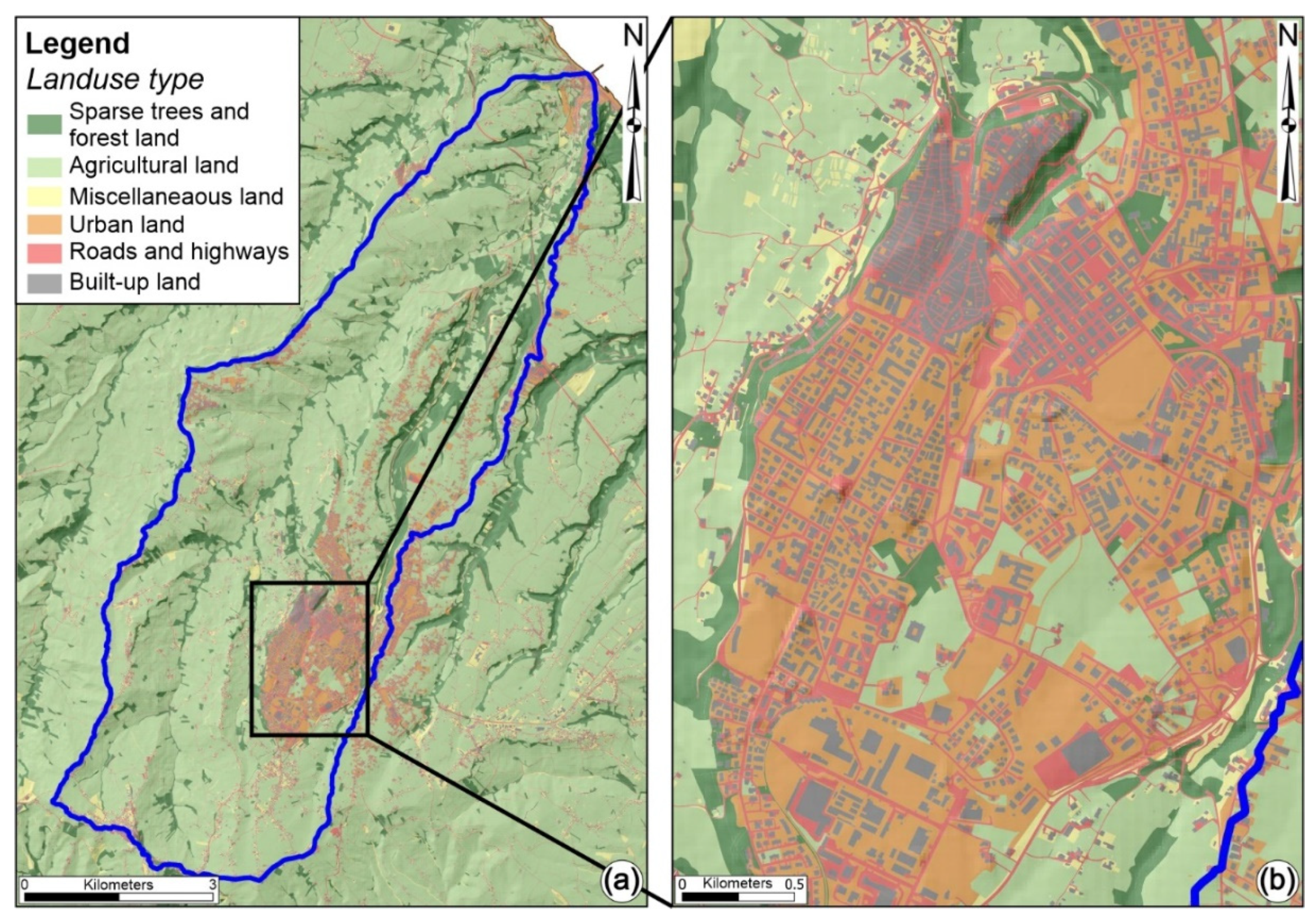
Morphometric and slope analysis was carried out with GIS software (QGIS 2018 [61]). This was based on the evaluation of the main orographic features, such as elevation and slope (calculated as the first derivate of elevation [62,63]). The hydrographic analysis was based on the detailed definition of the stream network and basins. Basin boundaries and streams were extracted automatically from the 10 m DTM, using Grass GIS 7.6.1, and verified through 1:5000 air-photos and 1 m LiDAR data. A specific investigation focused on the urban area of Lanciano, which allowed for the definition of the superficial urban streams and sub-basins. The study area was classified into 15 sub-basins, of which basic morphometric parameters (such as area, perimeter, relief, length, average slope) were obtained from the 10 m DTM.

3.2. Heavy Rainfall Analysis

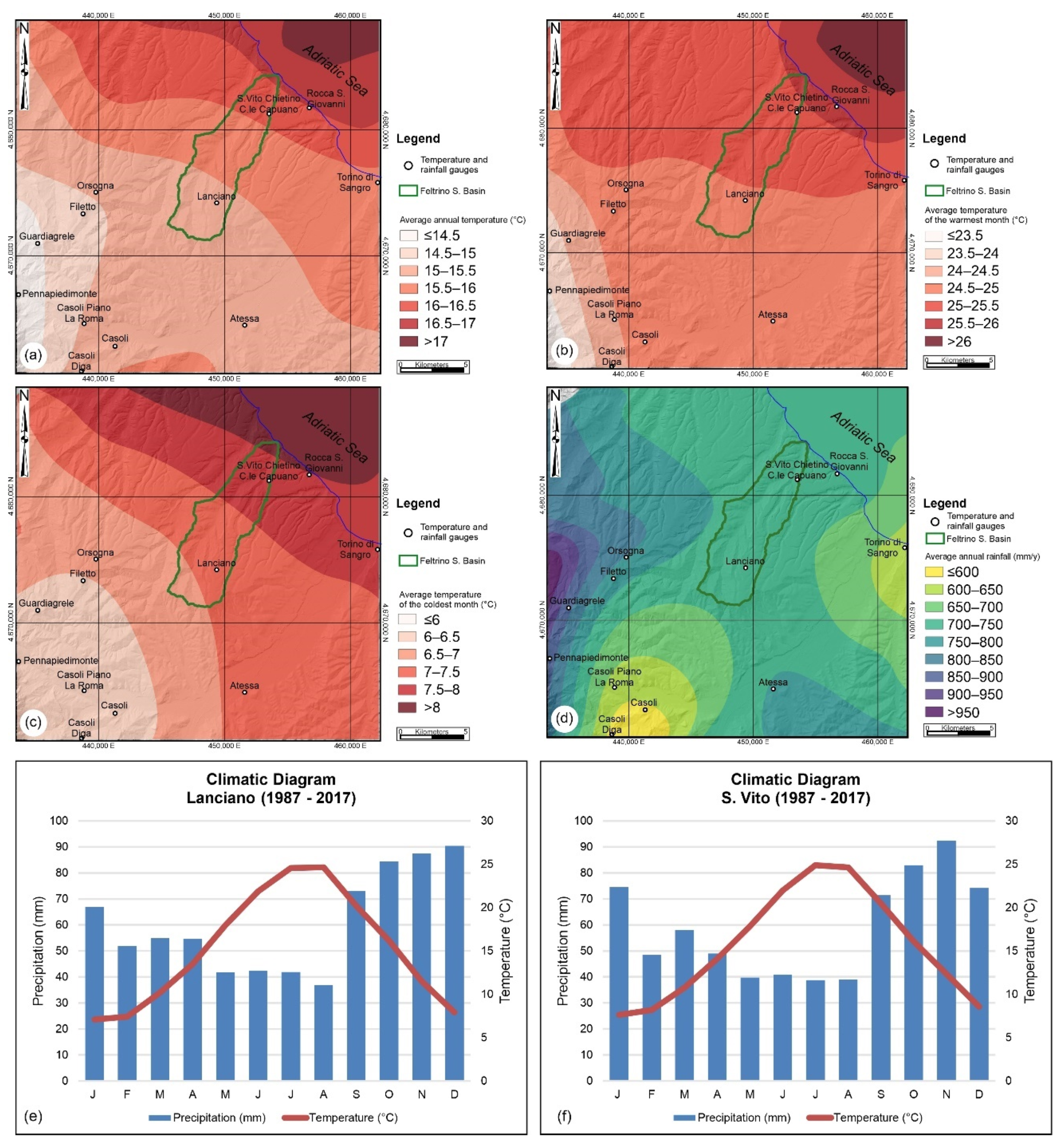
The analysis of heavy rainfall data was based on a rainfall dataset obtained from a network of 13 gauges (Table 2 and white dots in Figure 2 and Figure 4; data provided by the Functional Center and Hydrographic Office of the Abruzzo Region). Using the ArcGIS [64] Kernel Interpolation function, the variation of the distribution of temperature and rainfall in the study area was derived for a 30-year time record (1987–2017). From the dataset of each gauge, the average maximum rainfall over 1 h and 24 h were extracted (calculated as the average of the maximum rainfall event for each year of the dataset over 1 h and 24 h, respectively). For the rainfall gauges falling within the Feltrino Stream basin (Lanciano, S. Vito Chietino, and S. Vito–C.le Capuano stations), the climatic and maximum precipitation (1 h and 24 h) diagrams were extracted (considering all the historical dataset; Table 2). Moreover, the distribution and trends of intense daily rainfall events were investigated (i.e., the daily rainfall in the 99th percentile of time series, considering only rain days ≥1 mm/day) [65,66,67,68,69]. The return period of the heavy precipitation was derived for the Lanciano station dataset through the Gumbel and lognormal distributions [70].
Furthermore, the dataset of a hydrometric station located in the Feltrino Stream (Table 2 and blue dot in Figure 4) was analyzed to infer the response of the stream level to heavy rainfall events and the related time of concentration (Tc) [69]. Tc is the time lasting from the peak of rainfall distribution in an intense event and the related peak of river water level, possibly inducing a flood event. It is a useful data to understand the possible warning time from a rainfall event to the connected flood events. This value could also be very low in small hilly catchments as the Feltrino Stream basin.
Specifically, the Tc was estimated using the following empirical equation, defined by Carter [71]:
Tc = 0.0015476 × L0.6 × S–0.3,
where L is the length of the basin along the main channel from the hydraulically most distant point to the outlet (m), and S is the average slope of the basin (m/m).
The Tc was also verified through the rainfall and river level hydrograph, by comparing the time-shifting of the maximum values in the rainfall curve and the Feltrino Stream hydrographic level.

3.3. Geomorphological and Stream Network Analysis

Existing data regarding the geology, geomorphology, and flood hazard of the study area were retrieved from public authorities’ technical reports and scientific publications. Specifically, geological and geomorphological data were supplied by Seismic Microzonation of the Municipality of Lanciano [60], the Abruzzo-Sangro Basin Authority [48], and Piacentini et al. [33]. Flood hazard data were provided by the Abruzzo-Sangro Basin Authority [58] and reports of flooded areas by GNDCI [72] and the Municipality of Lanciano [59]. These data were integrated and verified through detailed geomorphological fieldwork (at the 1:5000–1:1000 scale) and stereoscopy air-photo interpretation, using 1:33,000- and 1:10,000-scale stereoscopic air-photos (Flight GAI 1954 and Flight Abruzzo Region 1981–1987), as well as analysis of 1:5000-scale orthophoto color images (2010).
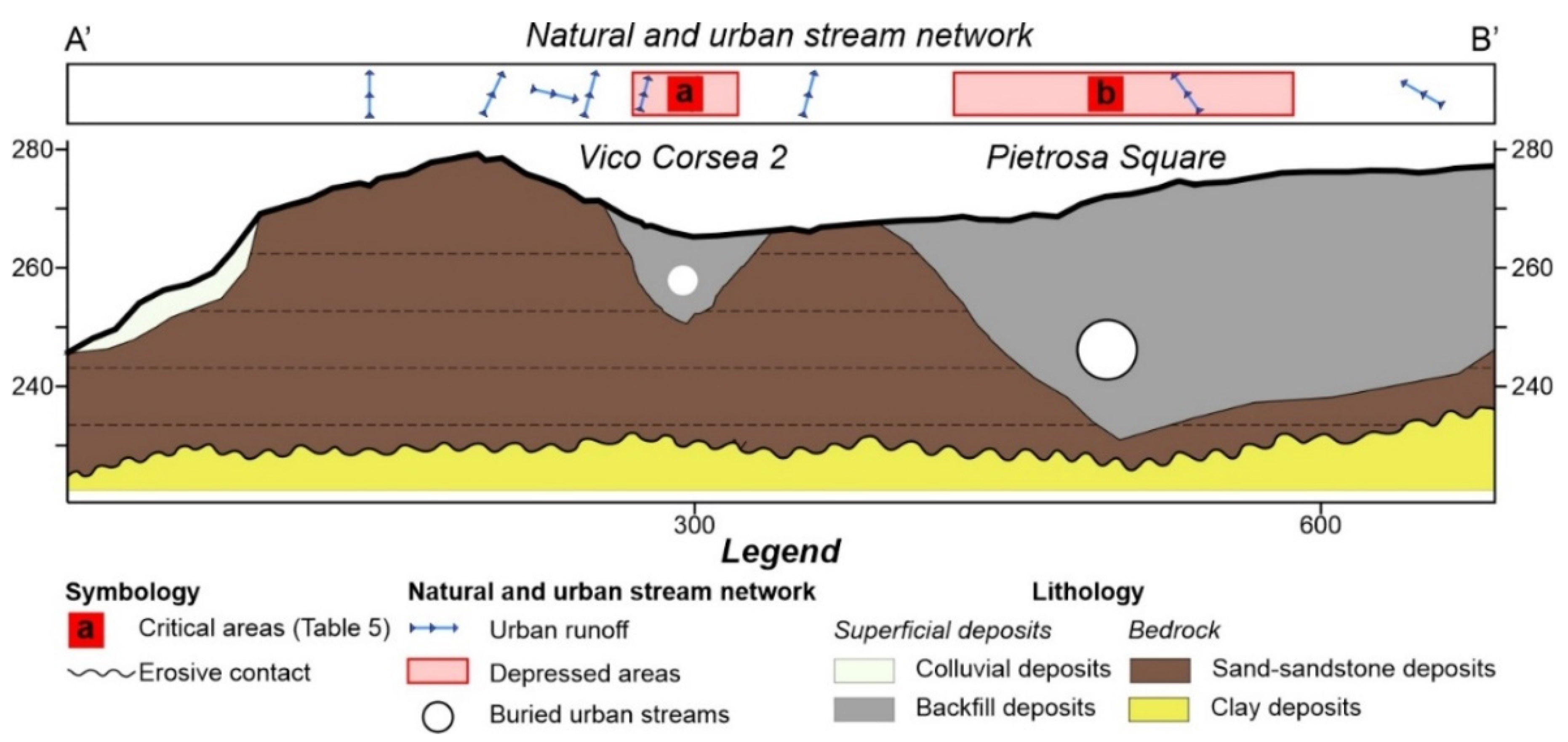
Furthermore, a detailed geomorphological analysis of the superficial and underground drainage network (i.e., urban channelized networks) of the urban area of Lanciano was performed, which allowed the evaluation of the influence of the actual urban streams in the local flood processes. First, we extracted the drainage network from the Regional Technical Maps of the Abruzzo Region, in which the drainage lines were divided into main and secondary, and into natural and artificial streams. These drainage lines were verified using cadastral maps, high-resolution aerial photos with 1 m resolution, and LiDAR data. Then, the whole urban area of Lanciano was examined through a detailed field survey. The superficial streams and runoff drainage lines (defined as surface runoff lines) and the underground urban streams were identified in the field and mapped, as well as the depressed areas already affected by flooding. Unfortunately, only the main buried features were mapped (approximately in some cases), while it was not possible to investigate channel sizes and diameters in detail. Finally, all bridges, underpasses, and raceways were analyzed by field surveys and mapped, defining the underbridge streams.

3.4. Flood Modeling

Hydrological modeling aims to highlight the flood-affected areas and simulate the amounts of streamflow generated by extreme precipitation events. The hydrological models compute the extreme events by taking into consideration the time series of precipitation data, topography, soil type, and land-use conditions [73,74,75]. The hydraulic models are used to compute streamflow conditions such as flow velocity, flow depth, and inundation areas. FLO-2D is a software tool primarily used for this purpose in different geomorphological and climatic contexts [76,77,78,79,80,81]. It is raster-based and allows for flexible geometry of the channel and the floodplain terrain. The model numerically routes a rainfall hydrograph while predicting the area of inundation and simulating flood wave attenuation. The model simulates the progression of the flood hydrograph, conserving flow volume, over a system of square grid elements representing topography and flow roughness [73,82].
In this case, the flood simulation was carried out through FLO-2D and focused on heavy rainfall events and the modeling of inundation areas and flow depth. It was based on elevation, roughness, and rainfall distribution parameters, while the contributions of evapotranspiration and infiltration were neglected since they can be considered very low in short-term heavy events, specifically in basins characterized by impermeable lithologies (clays), where a quick saturation of the soil occurs [83,84,85,86]. The discharge due to the buried stream network and sewage system was also neglected due to the weak data available (e.g., channels’ diameters, conveyance capacity) and to be cautious in considering the worst conditions. Specifically, the procedure was developed as follows. Initially, a DTM (Digital Terrain Model) was used to represent the area of interest (Feltrino drainage basin). For this purpose, a 10 m DTM and LiDAR (Light Detection and Ranging) data (for the valley bottom areas, resampled at 10 m) were combined and imported into the software, with a 10 m grid defined for this simulation. The flow roughness values (Manning’s –n [77]), were assigned according to the different land-use types, derived from the 1:5000 scale Numerical Topographic Database (Table 3). The rainfall amount and distribution were derived from the heavy rainfall analyses.
Furthermore, a detailed simulation of the urban area of Lanciano was performed. In this simulation, due to the lack of LiDAR data in the Lanciano area, the 5 m DTM was used, and a 5 m cell size was set for the model. Two rainfall distributions were used for the simulations, according to the significant rainfall events that occurred in recent decades. One is one day long and moderately intense; the second is a few hours long and more intense. More specifically, the following events were used: (1) a 24 h long event with a total rainfall of 110 mm and moderate intensity (5–10 mm/h) and the highest at the middle hours (representing the 2015 heavy rainfall event, which occurred in the area); (2) a 4 h long event with a total rainfall of 75 mm and a high-intensity spike (55 mm/h) in the second hour (representing the 2018 event, which occurred in Lanciano).
The numerical model provided the maximum flow depth, and this parameter was used to identify the expected flood areas in the basin and to verify the previous geomorphological data and the field investigations of critical areas.

3.5. Geodatabase and Critical Areas Assessment for Urban EWS

This stepwise analysis led to the definition of a multilayer geodatabase with geological, geomorphological, and hydrographic and hydrological data, which was the basis for the flood critical area assessment. The flood critical areas were defined through the analysis and overlay, supplemented using GIS software, of the data collected in the geodatabase. All the data were defined as polygon features, and linear features were buffered (5 m per side). An expert-based analysis of the overlaid data [87,88,89,90] allowed the design of a geomorphology-based matrix, which defined the criteria for the definition of the critical areas categories (low, moderate, and high). This matrix and the derived categories are not intended to represent a susceptibility or hazard distribution. They are aimed at the recognition of critical areas as possibly affected by flooding during heavy rainfall events, which have to be taken into account for alerting and civil protection purposes and actions. The combination of datasets provided by detailed fieldwork and flood modeling (direct investigations), and flood events and hazard datasets from previous investigations (indirect analysis), through the matrix, allowed the derivation of the map of the flood critical areas. Specifically, it was compiled by overlaying flood hazard maps [58], filings and reports of floods [59,72], detailed field surveys of previously flooded areas, detailed mapping of the drainage network, and data derived from the hydrological modeling. The field survey and mapping supported the definition of critical sites and the verification of the modeling. Finally, all the collected data were integrated into the GIS software through a cartographic overlay process in order to portray the spatial distribution of the flood critical areas.
The assessment of the main critical areas was the basis for implementing a real-time flood gauge and sensors network in the municipality of Lanciano. This urban network was set with the installation of measuring instruments (temperature–rainfall gauges, weather stations, hydrometers, flooding gauges) and the connection of existing ones (i.e., weather gauges, etc.). It is also able to integrate other types of sensors (e.g., inclinometers, landslide monitoring systems, anemometers, etc.), allowing for the implementations of new types of warnings. This network integrates at the urban and drainage basin-scale, the regional meteorological one (Functional Center and Hydrographic Office of the Abruzzo Region), which already exists in the area. The positioning and arrangement of the gauge network were strictly based on the official hazard areas [58], on the analysis of the basin-scale/urban critical areas defined in the Lanciano area, and on detailed direct field observations. This network allowed us to set up an EWS that can respond to local needs and can support the existing regional one (Allarmeteo) and the planned national one (ITallert).

4. Results

4.1. Heavy Rainfall Events

The analysis of the heavy rainfall events was based on the distribution of maximum rainfall (1 h and 24 h) and on the definition of the intense rainfall events (those above the 99th percentile of the rainfall distribution; i.e., 55 mm/day in this case).
The distribution of the average maximum rainfall over 1 h for each year of the dataset reveals the highest values in the W sector (~40 mm), with lower values in the SW and NE sectors (~24 mm) (Figure 5a). The Feltrino basin features values between 32 mm (inner part) and 24 mm (coastal area). The distribution of the average maximum rainfall over 24 h for each year of the dataset shows values between ~93 mm (W sector, Guardiagrele, and SE sector, Atessa), 63–66 mm (coastal area, E sector, Torino di Sangro), and ~60 mm (SW sector, Casoli) (Figure 5b). The Feltrino basin shows values of 75–84 mm.
The values of the maximum rainfall over 1 h in each year of the series show moderate-to-high values ranging from ~10 to ~75 mm and from ~10 to ~50 mm for the Lanciano and S. Vito gauges (blue histogram, Figure 5c,d), respectively. The values of the maximum rainfall in 24 h are from ~40 to ~210 mm (return period 2 and 200 years) and from ~25 to ~130 mm, respectively (orange histogram, Figure 5c,d).
The temporal distribution of the intense rainfalls events, in terms of the number and daily rainfall, was explicitly defined for the Lanciano (1974–2013) and S. Vito gauges (1974–2006 S. Vito Chietino; 2007–2017 S. Vito–C.le Capuano) (Figure 5e,f). The number of intense rainfall events (>55 mm/day) per year is from 0 to 6 for the Lanciano gauge and from 0 to 4 for the S. Vito gauge (orange line in Figure 5e,f). The maximum daily rainfall value in 24 h for each year, which exceeds the 99th percentile, is 131 mm (21 October 1994; return period ~15 years) and 130 mm (14 September 2012) for the Lanciano and S. Vito gauges, respectively (blue dots in Figure 5e,f). The trend of these values is not univocal in the two gauges.
The main historical and recent heavy rainfall events (Figure 5e,f) are for the 70% corresponding (in the range 1992 to present) to the main flood–landslide events (see Table 1). This confirmed the suitability of the identification of the heavy rainfall events. The most recent events were analyzed in detail (i.e., March 2015 and June 2018). The 2015 event represents a basin-scale event, with floods reported especially near the sea mouth. Moreover, this event induced widespread landslides (more than 70) throughout the Feltrino Stream basin. The 2018 event is a local one and caused major urban flash floods throughout the municipality of Lanciano and damage in the city center.
The return periods of the precipitation from 1 h to 24 h were calculated from the Lanciano precipitation time series (through the Gumbel distribution and the lognormal distribution; Figure 5g,h).

4.1.1. 5 March 2015 Basin-Scale Events

The March 2015 heavy rainfall event affected, for a moderately short time (about 24 h), the Feltrino Stream basin (data were recorded only in the S. Vito–C.le Capuano station due to technical reasons), especially on 5 March. This event, characterized by a cumulative rainfall of ~110 mm, occurred after another rainfall event (~80 mm on 25–26 February) for a total cumulative rainfall of ~190 mm in 1 week (Figure 6a). The rainfall intensity was moderate (i.e., 5–10 mm/h) with an almost regular increase and decrease (Figure 6b). The return period of this event (110 mm/24 h) was short (7 years, Figure 5g,h). A heavy rainfall event with these characteristics (rainfalls ≥100 mm over 24 h) was recorded 9 times over a 43-year time series (Figure 5f). The time of concentration (Tc), from the S. Vito–C.le Capuano station to the Feltrino–S. Vito hydrometric gauge, was empirically calculated to be ~46 min. This value is short due to the small basin size and was confirmed by the shifting of the hourly/cumulative rainfall and hydrographic level graphs for this event (Figure 6c).
The main effects of this event were found mainly in the area near the sea, where the river broke out of the banks and flooded roads, parks, parking lots, and even a camping site. Milder damage was also found in the innermost areas (Figure 7). During this event, a large number of landslides and soil erosion landforms were also induced in the whole basin. In particular, the landslide inventory contained 71 landslides covering a total surface area of 2.13 km2 (4.91% as soil erosion processes, 93.36% as small landslides, and 3.27% as large rotational landslides), which affected mainly superficial deposits.

4.1.2. 22 June 2018 Urban Flood Event

On 22 June 2018, a heavy rainfall event affected, for a short time (~4 h), the Feltrino Stream basin, and especially the municipality of Lanciano. This event was characterized by a cumulative rainfall of ~75 mm in 4 h but was highly concentrated (~55 mm in 1 h and ~68 mm in 3 h, from 16:00 to 19:00; Figure 8a) in the Lanciano area. The return period of this event was from 30 years (55 mm/1 h) to 16 years (75 mm/4 h; Figure 5g,h). Moderate rainfall occurred on the coastal area of the Feltrino basin (~5 mm/h with a cumulative ~17 mm, S. Vito; Figure 8b). A storm with these characteristics (rainfall ≥55 mm in 1 h) was recorded at least 8 times over the 86-year time series (Figure 5c). The time of concentration (Tc), from the Lanciano rainfall gauge to the Feltrino–S. Vito hydrometric gauge was empirically calculated to be ~70 min. Tc from the S. Vito–C.le Capuano to the Feltrino–S. Vito hydrometric gauges resulted in ~46 min. These values are short due to the small basin size and were confirmed by the shifting of the hourly/cumulative rainfall and hydrographic level graphs for this event (Figure 8). The graph outlines Tc = ~2 h from the Lanciano rainfall gauge to the Feltrino–S. Vito hydrometric gauge, and Tc = ~1 h from the S. Vito–C.le Capuano rainfall gauge to the Feltrino–S. Vito hydrometric gauge. For this event, the Tc values confirm the typical characteristics of a flash flood.
These extreme rain events induced excessive surface runoff, especially in impervious areas such as the urban areas, inducing flooding of underpasses and roads, with some stranded cars (Figure 9). Furthermore, the sewer system, undersized to dispose of such remarkable flows, was damaged in many areas, and rainwater mixed with sewage sludge overflowed from the maintenance holes. Finally, other effects, such as damaged roads and retaining walls, landslides, and mudflows along the roads, were also reported.

4.2. Natural and Urban Stream Network

The detailed analysis of the superficial hydrography allowed us to divide the Feltrino Stream catchment into 15 sub-basins (1–15, Table 4 and Figure 10). The main morphometric features show an area from several square kilometers (~20 km2) to some 0.01 square kilometers (0.018 km2). The elevation ranges from ~400 m a.s.l. in the inner part to sea level, showing relief values from 288 m (basin 7) to 19 m (basin 12). The average slope shows low values (from 3% to 8%) with some sub-basins with values up to ca. 10% (Table 4). For each sub-basin, the urbanized, semi-urbanized, and natural areas were defined. Some of them (sub-basins from 9 to 15) are highly urbanized (from ~45% to 100% of the sub-basins is covered by urban areas) and incorporate the urban area of Lanciano. In the urban area, the superficial streams are connected to buried urban streams, to the urban drainage and sewage system. These urban systems have been built over more than one century, and the specific sizes and diameters are mostly unknown.
For each of the sub-basins, the detailed field survey of the actual urban runoff features, integrated with the analysis of buried urban stream distribution and the historical and recently flooded sites, allowed us to define the convergence of surface runoff into six urban critical areas (a–f, Table 5 and Figure 10c). These are located in the urban area of Lanciano at an elevation ranging from 240 to 315 m a.s.l. Furthermore, they were divided into categories according to the natural and urban stream network features (i.e., depressed areas (b, c, d, f), buried urban streams (a, b, d, e), etc., Table 5).
As an example, one of the main critical areas in the historical center of Lanciano (Vico Corsea 2; Figure 10d; a in Table 5) is a closed depression ~7 m deep (from ~270 to 263.4 m a.s.l.) where all of the surrounding streets and related urban runoff converge. The draining system cannot cope with the discharge that occurs during heavy rainfall, and the site is frequently flooded (Figure 9b). Another particular case (Pietrosa Square; b in Table 5) is a depression ~15 m deep, with steep slopes. Below this site, the ancient course of the Pietrosa Stream flows in a buried urban stream. Backfill deposits buried the original valley for more than 30 m. This stream course (sub-basin 14) flows into a buried urban stream below the city center of Lanciano (sub-basin 11 and 12) and flows out in the northern part of the urban area, inside the Malsano Stream, connecting sub-basin 14 with sub-basin 10 and 8.
This investigation outlined how the water circulation of the urban center of Lanciano is strongly linked to the anthropic changes, which has intensely modified the urban landscape of the city. Specifically, large thicknesses of backfill deposits buried ancient valleys and streams, which were replaced by buried urban streams (Figure 11). For this reason, the urban hydrography of Lanciano is connected to the interaction of the superficial stream network with buried streams, which has led to various critical situations (Table 5). This specific analysis allowed us to integrate the official flood hazard map [58] on an urban scale and to define other critical areas, also in the urban area, which otherwise would not have been considered.

4.3. Flood Modeling

The 2D flood modeling using the FLO-2D tool was performed to verify, validate, and integrate the critical areas for flooding in the study area and specifically in the Lanciano urban area. The modeling was based on: (1) elevation data derived from DTMs; (2) land-use input data, used for the flow roughness values, derived from the Numerical Topographical Database (Table 3 and Figure 12); and (3) two different daily rainfall distributions derived from the heavy rainfall analyses (Figure 13). Rainfall distribution 1 shows 110 mm over 24 h with a maximum intensity of ~10 mm/h in the mid of the distribution (return period 7 years; Figure 13a); rainfall distribution 2 shows 75 mm over 4 h (return period 16 years) and a maximum intensity spike of 55 mm/h in the second hour (return period 30 years; Figure 13b).
For the Lanciano area, although the superficial stream network is connected to the buried streams, the precise size, diameter, and conveyance capacity are poorly known. For this reason, in order to be very cautious, considering the extreme worst situation of no discharge from the buried streams and sewage system, their discharge contribution was not considered in the modeling.
The first modeling was realized for the entire Feltrino Stream basin, using the 10 m DTM (resulting from the merging and resampling of the DTM of the basin and the LiDAR data of the valley axis) and the first rainfall distribution curve (Figure 13a). The results of this simulation show the expected flooding areas and the related flow depth (classified from 0.1 m to >1.5 m; Figure 14). The high values of water depth (from 1.0–1.5 to >1.5) are along the main valley of the Feltrino Stream, especially near the sea mouth, and in some sites of the Lanciano urban area. Low values of flow depth (from 0.1–0.5 to 0.5–1.0) are along the secondary valleys and in the depression of the Lanciano area. The high values along the main valley almost correspond to the regional hazard areas provided by the Abruzzo Region [58], and this supported the verifying and calibration of the model. Moreover, the flow depth values (from low to high) along the upper part of the main valley and along the minor streams provide a local scale integration of the regional data. To improve the local scale integration for the urban area of Lanciano, a second more detailed simulation was performed.
The second simulation was carried out in the urban area of Lanciano in order to better verify the urban flood critical areas. Due to the lack of LiDAR data in the Lanciano area, the simulation (with 5 m as cell size) was based on elevation data derived from the 5 m DTM and again on the roughness derived from the land-use data (Table 3 and Figure 12b). In this case, the intense rainfall simulation was run with two different rainfall distribution curves, according to two types of significant intense rainfall events. In the first scenario, where the first rainfall curve (moderate intensity, 24 h duration, Figure 13a) was used, several areas resulted in being affected by floods, also confirming the urban critical areas of Table 5. The highest value of water depth was 1.7 m and was found near Pietrosa Square and the Commercial area (b and d in Table 5 and Figure 15a). For the second scenario, the second rainfall curve (high intensity, 4 h duration, Figure 13b) was used. In this case, the distribution of the simulated flooded areas was very similar to the first simulation but with a higher value of water depth (~3.3 m). In general, the flow depth is higher than in the first scenario, indicating that higher intensity might produce more severe effects in urban areas. Moreover, the highest values of water depth were in areas corresponding to the a, b, d, and e urban critical areas (Table 5 and Figure 15b). This allowed us to validate the distribution of critical areas defined from the field geomorphological analysis and contributed to the calibration of the modeling.

4.4. Flood Critical Areas

The critical areas were assessed by analyzing, overlaying, and reclassifying the geomorphological–hydrographical data included in the geodatabase through the geomorphology-based matrix (Table 6) according to the spatial distribution and relationships between the factors involved in flood processes. In detail, the assessment was based on the overlaying and expert-based judgment of pre-existing hazard data [58] and reports of floods [59,72], plus new detailed field-based maps of geomorphological-stream network features, and water depth derived from hydrological flood modeling carried out for this work. Three categories of critical areas (low, moderate, and high) were defined, representing the map of the critical areas of the Feltrino basin (Figure 16a) and the Lanciano area (Figure 16b).
The criteria for the assessment of flood critical areas are defined in Table 6. Where one of the conditions or combinations of conditions defined in the columns one to four of the matrix occurs, then the category of the critical area is defined in column five. More specifically, Low (C1) critical areas include the lowest flood hazard areas [58], areas where secondary streams are present, expected flow depth in the range 0.1–1 m, and areas where no previous flood events were reported. Moderate (C2) critical areas include areas with medium-high values of flood hazard [58], main streams and urban runoff, and areas with no reports of previous floods; moreover, in this category, areas with expected flow depth in the range 0.1–1 m with reports of floods, and areas with flow depth in the range 1–1.5 m with no reports of floods were included. Finally, high (C3) critical areas are those in which past floods events are reported [59,72], a very high flood hazard class [58] is present, and depressed areas, underbridge streams, and buried urban streams are present. In this category, areas with modeled flow depths of 1–1.5 m and reports of flooded areas, and areas with modeled flow depths > 1.5 m were included.
The map shows that 6.38% (3.270 km2), 11.34% (5.813 km2), and 1.61% (0.823 km2) of the Feltrino Stream basin were classified as “low (C1)”, “moderate (C2)”, and “high (C3)” critical areas, respectively. In the Lanciano area, low critical areas (C1) comprise 4.09% (0.178 km2), moderate critical areas (C2) cover 9.11% (0.396 km2), and high critical areas (C3) include 2.95% (0.128 km2) of the overall urban area (Figure 16b). The very high flood critical areas were shown to be along the main watercourse of the Feltrino Stream, especially in its lowest reach (e.g., downstream the main confluence west from S. Vito) and where the river features a wide alluvial plain, near the river mouth. This area indeed suffered several flood events in recent historical times. Very high flood critical areas are also defined in the Lanciano urban area. These areas are derived from the signaling of urban flooded areas combined with the new data regarding the urban drainage network features and the flood modeling provided by this investigation.

5. Urban Gauge Network and EWS for Critical Areas Management

Based on the analysis of the critical areas defined in the urban area of Lanciano and in the Feltrino Stream basin, a network of gauges for supporting the management of the critical areas through an EWS was arranged. This network is composed of nine gauges and stations, communicating via a gateway (Table 7 and Figure 17), with the aim supporting at the urban-scale the regional gauge network (Functional Center and Hydrographic Office of the Abruzzo Region) and the regional-scale alerting system (Allarmeteo).
All the gauges are based on the Internet of Things (IoT) technology, defined as “a network of Internet-connected objects able to collect and exchange data.” Each communication is fully encrypted with three keys, each one with a length of 128 bits (algorithm AES-128, NIST approved and widely adopted as a best security practice for constrained nodes and networks). The sensors have a long-range of transmission (up to 15 km), and very low power consumption (sleep mode < 15uW–battery life > 1 year).
The network includes four weather stations or rainfall gauges (WS1, WS2, WS3, and RS1) measuring wind speed and direction, temperature, relative humidity, and rain–Range 0–10000 mm × 102/h; powered by solar energy panels), suitably located upstream, in the center, and downstream from the urban area of Lanciano. These gauges are arranged to monitor and track the intense rainfall events in real-time through the Lanciano area, providing rainfall threshold-based warnings, and to also support other measurements such as high wind and ice [93]. The rainfall thresholds were defined for the hourly and daily rainfall at two levels according to the analysis of the Lanciano and San Vito stations dataset. The hourly thresholds were defined at 20 mm/h and 40 mm/h (calculated as an hourly projection every 10 min), and the daily threshold were defined at 50 mm/day and 100 mm/h (Table 8). Two hydrometers (Hg1 and Hg2–Contactless Ultrasonic Sensor–Range 0–6 m +/− 1 mm, powered by solar panels) are located along the Feltrino Stream, one in the Lanciano area, in the upper-middle course of the stream, and the other in the S. Vito area, near the sea mouth. They are placed to check the response of the main watercourse to rainfall events and the relative time of concentration (Tc). Three flood gauges (LFS1, LFS2, and LFS3–immersion sensor with 2 thresholds 0–50 mm / 100–150 mm, battery-powered) are located in the main flood critical areas within the city center. They provide real-time notification of the water level in these specific sites during rainfall events. These sensors will be connected to traffic lights to automatically block access to critical areas and roads when detecting a flood event, taking into account that roads are the main transport infrastructure in the area. The gateway connects the sensors, and it is composed of up to 8 uplink/downlink independent channels LoRaWan, GPS clock timing sync, and LoRa Alliance for EU 863-870 MHz. It has a TCP/IP connection through ethernet or via 4G connection. All the thresholds will be verified in the first year of running the system.
The EWS is the result of the integration of sensor gauges and critical areas, based on official hazard data, integrated with local geomorphological surveys and flood modeling, and is connected to the regional alerting system (Allarmeteo). This system, thus structured, is based on forecast-based information and real-time data (especially the amount of rainfall, the water level in critical areas, and the main river) for the alerting of critical areas. More specifically, the system is based on three levels of alert/alarm input: (1) forecast-based alerting bulletins provided by Allarmeteo (regional warning system); (2) passing of rainfall thresholds (measured in real-time by the sensors) based on the previous floods and statistical analysis of rainfall dataset, and in agreement with existing studies regarding the study area [10,53,91] (the verification and calibration of the rainfall thresholds is ongoing and will be improved in the early stages of the EWS activity); (3) water level increase measured in real-time in the main flood critical areas within the city center. These inputs and the overall system provide different levels of alert/alarm and flood critical areas scenarios to the municipal civil protection for the management of the heavy rainfall events. The system is supported by a mobile application for smartphones, exploiting the inbuilt geolocalization features and communication tools of recent smartphones, and available for different targets of users. It will provide different levels of real-time communication tools (1) for decision-makers and civil protection management and (2) for communication to the citizens and the general public. According to the municipal Civil Protection Plan, simple, clear, and useful warning messages will support decision-makers and citizens to handle critical events and manage critical areas.

6. Conclusions

Heavy rainfall events, combined with increasing urbanization and related land use, landscape, and stream changes, make urban areas prone to flash floods. This is primarily expected in big cities but is also increasingly common in moderate–small towns and in hilly areas (such as those surrounding the Apennines chain in Italy), which places inhabitants at risk and causes heavy material losses. Flash floods are of a very fast onset, with a relatively short spike and rapid withdrawal [23,94,95]. Therefore, it is necessary to design adequate and smart adaptation measures to reduce the negative impact on society. To this purpose, EWSs, especially if strongly geomorphology-based, are recognized worldwide as one of the best tools aimed at risk prevention, mitigation, preparedness, and response strategies [96,97,98,99,100].
In this paper, we presented a multidisciplinary approach for the assessment of flood critical areas induced by heavy rainfall events and the emplacement of an EWS in the Feltrino Stream basin and, specifically, in the Lanciano urban area (hilly piedmont area of eastern central Apennines, Abruzzo Region). This approach includes an integrated basin-scale analysis based on (1) orography analysis; (2) heavy rainfall and hydrometric data analysis; (3) acquisition, verification, and validation of available geological, geomorphological, and hazard data; (4) new detailed geomorphological field mapping of the urban stream network; (5) validation of geomorphological analysis through 2D flood modeling with FLO-2D software. This stepwise analysis allowed us to define a complete geodatabase of the geographical, geological, geomorphological, and flood modeling data of the Feltrino basin and the Lanciano area. The analysis of the heavy rainfall events (as ≥55 mm/day) shows that these events have occurred from 0 to 6 times per year over the last few decades (rainfall up to 130 mm/day and 75 mm/h since 1974 and the heaviest event of 210 mm/day in 1947) and are highly consistent with the past flood–landslide heavy events (Table 1).
The overlay of official hazard data, stream geomorphological data, and flow depth values obtained by hydraulic modeling, led to the definition of different classes of flood critical areas through a geomorphology-based matrix. For the Feltrino Stream basin, low (6.38% of the basin area), moderate (11.34%), and high (1.61%) flood critical areas were identified and mapped. The Lanciano urban area features 4.09% of the low class, 9.11% of the moderate class, and 2.95% of the high class of critical areas. These critical areas are not intended to be a closed tool but are open to being continuously updated and verified following detailed hydrological analyses and after the occurrence of new events. The combination of the areal distribution of critical areas, the temporal distribution of intense rainfall events, and related flood historical/recent events provides evidence for the need for a local adaptation system in the area of Lanciano based on an urban EWS, integrated into a regional network of alerting systems.
The urban EWS was placed for the management of heavy rainfall and flash flood events. It combines the critical area scenarios and a network of nine gauges and stations (i.e., weather stations, rainfall gauges, hydrometers, flood level gauges) and a related communication system, whose arrangement is based on the geomorphological configuration of the Lanciano area, the distribution of the critical areas, and the past flood events. It integrates different types of gauges and incorporates the information derived from the regional forecast-based warning system (Allarmeteo), generating a web-cloud gauges network and communication system. These multiple alert/alarm inputs include regional forecast-based alerting, the passing of rainfall thresholds, and the water level increase measured by flooding sensors in real-time. This system provides new data to increase the detailed knowledge of the meteorological and geomorphological events, both at the basin scale and the urban scale, and to improve the mitigation of flood-related risks. It is supported by a specific application for smartphones, covers the monitoring of rainfall and flood events, the management of the critical areas, and the prevention/mitigation of the effects of heavy rainfall and flood events. The mobile application includes tools for providing forecast based alerting (from regional Allarmeteo), for civil protection communication and alarm management response in heavy rainfall events (before, during, and after events) at different levels and for different targets of users (decision-makers, civil protection managers, citizens, and the general public). It will also be useful for before-event dissemination and preparedness to flood risk and is expected to support municipal civil protection activities.
In conclusion, the overall results of this work are: (1) the provision of new data on the geomorphology–hydrography of the study area and the flood critical areas (specifically in the urban area of Lanciano), (2) the outline of a geomorphology-based methodological approach for the definition of flood critical areas and the configuration of an urban EWS, (3) the support of the set-up of a risk prevention system based on the integration of sensor–gauge data and critical scenarios, resulting from official hazard data, which must be taken into consideration by the municipalities for civil protection purposes, integrated with local investigations and civil protection plans, and (4) the provision of new tools for increasing the detailed knowledge of the meteorological and geomorphological heavy events in the Feltrino basin (at the basin scale and urban scale). The urban EWS is integrated with the regional alerting system network and is designed for local authorities’ communications and Civil Protection purposes, and for the management of critical areas during flood events, and will improve the mitigation of the related risks. Finally, this procedure can also be implemented for the analysis of landslides (and other natural processes such as wind, snow, etc.), considering the landslide hazard data, the reports of past events in the area, carrying out a specific landslide susceptibility analysis, and adding to the EWS landslide-monitoring sensors (e.g., inclinometers, piezometers, dilatometers, radar monitoring instruments, etc.). This study was designed explicitly for hilly landscapes in Apennines piedmont areas, which have experienced heavy flood events in the last decades, and can be easily replicated in similar watersheds and environments.

Author Contributions

Conceptualization, E.M., T.P. (Tommaso Piacentini), and F.B.; methodology, E.M., C.C., and T.P. (Tommaso Piacentini); data curation, E.M., and T.P. (Tommaso Piacentini); resources, F.B., C.G, A.P., and T.P. (Tommaso Pagliani); geomorphological investigation C.C., T.P. (Tommaso Piacentini), and V.M.; installation of monitoring system, C.G. and A.P.; GIS mapping, flood modeling, and writing—original draft preparation, C.C.; writing—review and editing, C.C., E.M., and T.P. (Tommaso Piacentini); validation and supervision E.M. and T.P (Tommaso Piacentini); project administration and funding acquisition, F.B., E.M., S.F., and T.P. (Tommaso Piacentini). All authors have read and agreed to the published version of the manuscript.

Funding

This research and the APC were funded by Lanciano Municipality to the Department of Engineering and Geology, Università degli Studi “G. d’Annunzio” Chieti-Pescara, within the Communicate to Protect—Lanciano project granted by the Abruzzo Region (FSE Abruzzo 2014-2020—Piano Operativo 2017–2019 Intervento n.37 “Comunicare per Proteggere”).

Acknowledgments

The authors are glad to thank the anonymous reviewers that helped to greatly improve the manuscript with their precious suggestions and comments. The authors wish to thank the Cartographic Office of the Abruzzo Region by means of the Open Geodata Portal (http://opendata.regione.abruzzo.it/), for providing the topographic data, 10 m Digital Terrain Model, aerial photos, and orthophotos used for this work; also thanks to the Ministero dell’Ambiente e della Tutela del Territorio e del Mare (http://www.minambiente.it/) for providing the LiDAR data. The rainfall data were provided by the Functional Center and Hydrographic Office of the Abruzzo Region (Centro Funzionale e Ufficio Idrografico Regione Abruzzo).

Conflicts of Interest

The authors declare no conflict of interest.

References

  1. Napolitano, E.; Marchesini, I.; Salvati, P.; Donnini, M.; Bianchi, C.; Guzzetti, F. LAND-deFeND–An innovative database structure for landslides and floods and their consequences. J. Environ. Manag. 2018, 207, 203–218. [Google Scholar] [CrossRef] [PubMed]
  2. Salvati, P.; Bianchi, C.; Fiorucci, F.; Giostrella, P.; Marchesini, I.; Guzzetti, F. Perception of flood and landslide risk in Italy: A preliminary analysis. Nat. Hazards Earth Syst. Sci. 2014, 14, 2589–2603. [Google Scholar] [CrossRef] [Green Version]
  3. Salvati, P.; Petrucci, O.; Rossi, M.; Bianchi, C.; Pasqua, A.A.; Guzzetti, F. Gender, age and circumstances analysis of flood and landslide fatalities in Italy. Sci. Total Environ. 2018, 610–611, 867–879. [Google Scholar] [CrossRef] [PubMed]
  4. Gariano, S.L.; Guzzetti, F. Landslides in a changing climate. Earth Sci. Rev. 2016, 162, 227–252. [Google Scholar] [CrossRef] [Green Version]
  5. Blöschl, G.; Hall, J.; Viglione, A.; Perdigão, R.A.P.; Parajka, J.; Merz, B.; Lun, D.; Arheimer, B.; Aronica, G.T.; Bilibashi, A.; et al. Changing climate both increases and decreases European river floods. Nature 2019, 573, 108–111. [Google Scholar] [CrossRef]
  6. Sharma, A.; Wasko, C.; Lettenmaier, D.P. If Precipitation Extremes Are Increasing, Why Aren’t Floods? Water Resour. Res. 2018, 54, 8545–8551. [Google Scholar] [CrossRef]
  7. Lehner, B.; Döll, P.; Alcamo, J.; Henrichs, T.; Kaspar, F. Estimating the impact of global change on flood and drought risks in Europe: A continental, integrated analysis. Clim. Chang. 2006, 75, 273–299. [Google Scholar] [CrossRef]
  8. Bufalini, M.; Farabollini, P.; Fuffa, E.; Materazzi, M.; Pambianchi, G.; Tromboni, M. The significance of recent and short pluviometric time series for the assessment of flood hazard in the context of climate change: Examples from some sample basins of the Adriatic Central Italy. AIMS Geosci. 2019, 5, 568–590. [Google Scholar] [CrossRef]
  9. Enigl, K.; Matulla, C.; Schlögl, M.; Schmid, F. Derivation of canonical total-sequences triggering landslides and floodings in complex terrain. Adv. Water Resour. 2019, 129, 178–188. [Google Scholar] [CrossRef]
  10. Ferretti, R.; Lombardi, A.; Tomassetti, B.; Sangelantoni, L.; Colaiuda, V.; Mazzarella, V.; Maiello, I.; Verdecchia, M.; Redaelli, G. Regional ensemble forecast for early warning system over small Apennine catchments on Central Italy. Hydrol. Earth Syst. Sci. Discuss. 2019, 1–25. [Google Scholar] [CrossRef] [Green Version]
  11. Lin, L.; Wu, Z.; Liang, Q. Urban flood susceptibility analysis using a GIS-based multi-criteria analysis framework. Nat. Hazards 2019, 97, 455–475. [Google Scholar] [CrossRef]
  12. Young, A.F. Urban expansion and environmental risk in the São Paulo Metropolitan Area. Clim. Res. 2013, 57, 73–80. [Google Scholar] [CrossRef] [Green Version]
  13. Nirupama, N.; Simonovic, S.P. Increase of flood risk due to urbanisation: A Canadian example. Nat. Hazards 2007, 40, 25–41. [Google Scholar] [CrossRef]
  14. Fordham, M. Participatory planning for flood mitigation: Models and approaches. In Floods; Taylor and Francis Inc.: London, UK, 2014; pp. 66–79. ISBN 9781315830889. [Google Scholar]
  15. Brath, A.; Montanari, A.; Moretti, G. Assessing the effects on flood risk of land-use changes in the last five decades: An Italian case study. IAHS-AISH Publ. 2003, 278, 435–441. [Google Scholar]
  16. Perales-Momparler, S.; Hernández-Crespo, C.; Vallés-Morán, F.; Martín, M.; Andrés-Doménech, I.; Andreu Álvarez, J.; Jefferies, C. SuDS efficiency during the start-up period under mediterranean climatic conditions. Clean Soil Air Water 2014, 2, 178–186. [Google Scholar] [CrossRef] [Green Version]
  17. Jha, A.K.; Bloch, R.; Lamond, J. Cities and Flooding: A Guide to Integrated Urban Flood Risk Management for the 21st Century; The World Bank: Washington, DC, USA, 2012. [Google Scholar] [CrossRef] [Green Version]
  18. Ramos, H.M.; Pérez-Sánchez, M.; Franco, A.B.; López-Jiménez, P.A. Urban floods adaptation and sustainable drainage measures. Fluids 2017, 2, 61. [Google Scholar] [CrossRef] [Green Version]
  19. Fowler, H.J.; Wilby, R.L. Detecting changes in seasonal precipitation extremes using regional climate model projections: Implications for managing fluvial flood risk. Water Resour. Res. 2010, 46, 1–17. [Google Scholar] [CrossRef] [Green Version]
  20. Trigila, A.; Iadanza, C.; Bussettini, M.; Lastoria, B. Dissesto Idrogeologico in Italia: Pericolosità e Indicatori Di rischio-Edizione 2018; ISPRA: Rome, Italy, 2018; ISBN 9788844809010. [Google Scholar]
  21. IRPI-CNR. Rapporto Periodico Sul Rischio Posto Alla Popolazione Italiana da Frane e Inondazioni; IRPI: Perugia, Italy, 2020; Available online: http://polaris.irpi.cnr.it/wp-content/uploads/report_2019.pdf (accessed on 20 February 2020).
  22. Hofmann, J.; Schüttrumpf, H. Risk-Based Early Warning System for Pluvial Flash Floods: Approaches and Foundations. Geosciences 2019, 9, 127. [Google Scholar] [CrossRef] [Green Version]
  23. Acosta-Coll, M.; Ballester-Merelo, F.; Martinez-Peiró, M.; De la Hoz-Franco, E. Real-time early warning system design for pluvial flash floods—A review. Sensors 2018, 18, 2255. [Google Scholar] [CrossRef] [Green Version]
  24. Ma, M.; Zhang, J.; Su, H.; Wang, D.; Wang, Z. Update of early warning indicators of flash floods: A case study of Hunjiang District, Northeastern China. Water 2019, 11, 314. [Google Scholar] [CrossRef] [Green Version]
  25. Corral, C.; Berenguer, M.; Sempere-Torres, D.; Poletti, L.; Silvestro, F.; Rebora, N. Comparison of two early warning systems for regional flash flood hazard forecasting. J. Hydrol. 2019, 572, 603–619. [Google Scholar] [CrossRef] [Green Version]
  26. Krzhizhanovskaya, V.V.; Shirshov, G.S.; Melnikova, N.B.; Belleman, R.G.; Rusadi, F.I.; Broekhuijsen, B.J.; Gouldby, B.P.; Lhomme, J.; Balis, B.; Bubak, M.; et al. Flood early warning system: Design, implementation and computational modules. Procedia Comput. Sci. 2011, 4, 106–115. [Google Scholar] [CrossRef] [Green Version]
  27. Pradhan, B. Flood susceptible mapping and risk area delineation using logistic regression, GIS and remote sensing. J. Spat. Hydrol. 2009, 9, 1–18. [Google Scholar]
  28. González-Cao, J.; García-Feal, O.; Fernández-Nóvoa, D.; Domínguez-Alonso, J.M.; Gómez-Gesteira, M. Towards an automatic early warning system of flood hazards based on precipitation forecast: The case of the Miño River (NW Spain). Nat. Hazards Earth Syst. Sci. 2019, 19, 2583–2595. [Google Scholar] [CrossRef] [Green Version]
  29. Orozco, M.M.; Caballero, J.M. Smart disaster prediction application using flood risk analytics towards sustainable climate action. In Proceedings of the MATEC Web of Conferences, Beijing, China, 25–27 May 2018. [Google Scholar] [CrossRef] [Green Version]
  30. De Castro, J.T.; Salistre, G.M.; Byun, Y.C.; Gerardo, B.D. Flash flood prediction model based on multiple regression analysis for decision support system. In Proceedings of the World Congress on Engineering and Computer Science (WCECS), San Francisco, CA, USA, 3–25 October 2013. [Google Scholar]
  31. Capparelli, G.; Versace, P. FLaIR and SUSHI: Two mathematical models for early warning of landslides induced by rainfall. Landslides 2011, 8, 67–79. [Google Scholar] [CrossRef]
  32. Miccadei, E.; Carabella, C.; Paglia, G.; Piacentini, T. Paleo-drainage network, morphotectonics, and fluvial terraces: Clues from the Verde Stream in the middle Sangro river (Central Italy). Geosciences 2018, 8, 337. [Google Scholar] [CrossRef] [Green Version]
  33. Piacentini, T.; Sciarra, M.; Miccadei, E.; Urbano, T. Near-surface deposits and hillslope evolution of the Adriatic piedmont of the Central Apennines (Feltrino Stream basin and minor coastal basins, Abruzzo, Italy). J. Maps 2015, 11, 299–313. [Google Scholar] [CrossRef] [Green Version]
  34. Ascione, A.; Cinque, A.; Miccadei, E.; Villani, F.; Berti, C. The Plio-Quaternary uplift of the Apennine chain: New data from the analysis of topography and river valleys in Central Italy. Geomorphology 2008, 102, 105–118. [Google Scholar] [CrossRef] [Green Version]
  35. Giano, S.I.; Giannandrea, P. Late Pleistocene differential uplift inferred from the analysis of fluvial terraces (southern Apennines, Italy). Geomorphology 2014, 217, 89–105. [Google Scholar] [CrossRef]
  36. D’Alessandro, L.; Miccadei, E.; Piacentini, T. Morphotectonic study of the lower Sangro River valley (Abruzzi, Central Italy). Geomorphology 2008, 102, 145–158. [Google Scholar] [CrossRef]
  37. Miccadei, E.; Piacentini, T.; Buccolini, M. Long-term geomorphological evolution in the Abruzzo area, Central Italy: Twenty years of research. Geol. Carpathica 2017, 68, 19–28. [Google Scholar] [CrossRef] [Green Version]
  38. Geurts, A.H.; Whittaker, A.C.; Gawthorpe, R.L.; Cowie, P.A. Transient landscape and stratigraphic responses to drainage integration in the actively extending central Italian Apennines. Geomorphology 2020, 353, 107013. [Google Scholar] [CrossRef]
  39. D’Alessandro, L.; Miccadei, E.; Piacentini, T. Morphostructural elements of central-eastern Abruzzi: Contributions to the study of the role of tectonics on the morphogenesis of the Apennine chain. Quat. Int. 2003, 101–102, 115–124. [Google Scholar] [CrossRef]
  40. Mayer, L.; Menichetti, M.; Nesci, O.; Savelli, D. Morphotectonic approach to the drainage analysis in the North Marche region, central Italy. Quat. Int. 2003, 101–102, 157–167. [Google Scholar] [CrossRef]
  41. Miccadei, E.; Piacentini, T.; Pozzo, A.D.; La Corte, M.; Sciarra, M. Morphotectonic map of the Aventino-Lower Sangro valley (Abruzzo, Italy), scale 1:50,000. J. Maps 2013, 9, 390–409. [Google Scholar] [CrossRef] [Green Version]
  42. Parlagreco, L.; Mascioli, F.; Miccadei, E.; Antonioli, F.; Gianolla, D.; Devoti, S.; Leoni, G.; Silenzi, S. New data on Holocene relative sea level along the Abruzzo coast (central Adriatic, Italy). Quat. Int. 2011, 232, 179–186. [Google Scholar] [CrossRef]
  43. Carabella, C.; Buccolini, M.; Galli, L.; Miccadei, E.; Paglia, G.; Piacentini, T. Geomorphological analysis of drainage changes in the NE Apennines piedmont area: The case of the middle Tavo River bend (Abruzzo, Central Italy). J. Maps 2020, 16, 222–235. [Google Scholar] [CrossRef] [Green Version]
  44. Piacentini, T.; Galli, A.; Marsala, V.; Miccadei, E. Analysis of soil erosion induced by heavy rainfall: A case study from the NE Abruzzo Hills Area in Central Italy. Water 2018, 10, 1314. [Google Scholar] [CrossRef] [Green Version]
  45. Calista, M.; Miccadei, E.; Pasculli, A.; Piacentini, T.; Sciarra, M.; Sciarra, N. Geomorphological features of the Montebello sul Sangro large landslide (Abruzzo, Central Italy). J. Maps 2016, 12, 882–891. [Google Scholar] [CrossRef] [Green Version]
  46. Calista, M.; Miccadei, E.; Piacentini, T.; Sciarra, N. Morphostructural, Meteorological and Seismic Factors Controlling Landslides in Weak Rocks: The Case Studies of Castelnuovo and Ponzano (North East Abruzzo, Central Italy). Geosciences 2019, 9, 122. [Google Scholar] [CrossRef] [Green Version]
  47. Bozzano, F.; Carabella, C.; De Pari, P.; Discenza, M.E.; Fantucci, R.; Mazzanti, P.; Miccadei, E.; Rocca, A.; Romano, S.; Sciarra, N. Geological and geomorphological analysis of a complex landslides system: The case of San Martino sulla Marruccina (Abruzzo, Central Italy). J. Maps 2020, 16, 126–136. [Google Scholar] [CrossRef] [Green Version]
  48. Abruzzo-Sangro Basin Authority. Geomorphological Map, Scale 1:25,000. Piano Stralcio di Bacino per l’Assetto Idrogeologico dei Bacini di Rilievo Regionale Abruzzesi e del Bacino del Fiume Sangro. (L.R. 18.05 1989 n.81 e L. 24.08.2001); Abruzzo Region: L’Aquila, Italy, 2005.
  49. Abruzzo-Sangro Basin Authority. Hydrogeological (PAI) Plan–Hazard Map, Scale 1:25,000. Piano Stralcio di Bacino per l’Assetto Idrogeologico dei Bacini di Rilievo Regionale Abruzzesi e del Bacino del Fiume Sangro. (L.R. 18.05 1989 n.81 e L. 24.08.2001); Abruzzo Region: L’Aquila, Italy, 2005.
  50. Miccadei, E.; Piacentini, T.; Gerbasi, F.; Daverio, F. Morphotectonic map of the Osento River basin (Abruzzo, Italy), scale 1:30,000. J. Maps 2012, 8, 62–73. [Google Scholar] [CrossRef]
  51. Peel, M.C.; Finlayson, B.L.; McMahon, T.A. Updated world map of the Köppen-Geiger climate classification. Hydrol. Earth Syst. 2007, 11, 1633–1644. [Google Scholar] [CrossRef] [Green Version]
  52. Di Lena, B.; Antenucci, F.; Mariani, L. Space and time evolution of the Abruzzo precipitation. Ital. J. Agrometeorol. 2012, 1, 5–20. [Google Scholar]
  53. Di Lena, B.; Antenucci, F.; Giuliani, D.; Rampa, C. Analisi Spazio Temporale Delle Precipitazioni Nella REGIONE Abruzzo; Regione Abruzzo-Direzione Politiche Agricole e di Sviluppo Rurale, Forestale, Caccia e Pesca, Emigrazione: Vasto, Italy, 2016; Available online: https://www.regione.abruzzo.it/system/files/agricoltura/agrometereologia/ATLANTE_PLUVIOMETRICO.pdf (accessed on 21 November 2019).
  54. Chiaudani, A.; Antenucci, F.; Di Lena, B. Historical analysis of maximum intensity precipitation (1, 3, 6, 12 hours) in Abruzzo Region (Italy)-Period 1951–2012. In Proceedings of the Agrometeorologia per la Sicurezza Ambientale ed Alimentare; Pàtron, Ed.; Ass. Italiana di Agrometeorologia (AIAM): Firenze, Italy, 2013. [Google Scholar]
  55. Costantini, E.A.C.; Fantappié, M.; L’Abate, G. Climate and pedoclimate of Italy. In The Soils of Italy. World Soils Book Series; Costantini, E., Dazzi, C., Eds.; Springer: Dordrecht, The Netherlands, 2013. [Google Scholar]
  56. Strahler, A.N. Quantitative classification of watershed geomorphology. Trans. Am. Geophys. Union 1957, 38, 913–920. [Google Scholar] [CrossRef] [Green Version]
  57. ISPRA. Geological Map of Italy, Scale 1:50,000, Sheet 361 “Chieti”; Servizio Geologico d’Italia: Rome, Italy, 2010. Available online: http://www.isprambiente.gov.it/Media/carg/361_CHIETI/Foglio.html (accessed on 21 November 2019).
  58. Abruzzo-Sangro Basin Authority. PSDA Plan–Hazard Map, Scale 1:25,000. Piano Stralcio di Bacino per l’Assetto Idrogeologico dei Bacini di Rilievo Regionale Abruzzesi e del Bacino del Fiume Sangro. (L.R. 18.05 1989 n.81 e L. 24.08.2001); Abruzzo Region: L’Aquila, Italy, 2005.
  59. Municipality of Lanciano. Piano Regolatore Generale–Relazione geologica–Comune di Lanciano; Municipality of Lanciano: Lanciano, Italy, 2008. [Google Scholar]
  60. Municipality of Lanciano. Studio di Microzonazione Sismica di I livello del Comune di Lanciano (CH), ai sensi dell’Art.11 della Legge 24 Giugno 2009, n. 77; Municipality of Lanciano: Lanciano, Italy, 2015; p. 92. [Google Scholar]
  61. QGIS Development Team. QGIS Geographic Information System, Version 3.4 “Madeira”. Open Source Geospatial Foundation Project. 2018. Available online: http://qgis.osgeo.org (accessed on 8 January 2019).
  62. Strahler, A.N. Dynamic basis of geomorphology. Bull. Geol. Soc. Am. 1952, 63, 923–938. [Google Scholar] [CrossRef]
  63. Burbank, D.W.; Anderson, R.S. Tectonic Geomorphology, 2nd ed.; Wiley, B., Ed.; John Wiley & Sons, Ltd.: Chichester, UK, 2011; ISBN 9781444338867. [Google Scholar]
  64. ESRI. ArcGIS Desktop: Release 10.6; Environmental Systems Research Institute: Redlands, CA, USA, 2018. [Google Scholar]
  65. Hov, Ø.; Cubasch, U.; Fischer, E.; Höppe, P.; Iversen, T.; Kvamstø, N.G.; Kundzewicz, Z.W.; Rezacova, D.; Rios, D.; Santos, F.D.; et al. Extreme Weather Events in Europe: Preparing for Climate Change Adaptation; Norwegian Meteorological Institute: Oslo, Norway, 2013.
  66. NOAA. U.S. Climate Extremes Index. Available online: www.ncdc.noaa.gov/extremes/cei (accessed on 8 January 2020).
  67. Schär, C.; Ban, N.; Fischer, E.M.; Rajczak, J.; Schmidli, J.; Frei, C.; Giorgi, F.; Karl, T.R.; Kendon, E.J.; Tank, A.M.G.K.; et al. Percentile indices for assessing changes in heavy precipitation events. Clim. Chang. 2016, 137, 201–216. [Google Scholar] [CrossRef] [Green Version]
  68. Myhre, G.; Alterskjær, K.; Stjern, C.W.; Hodnebrog; Marelle, L.; Samset, B.H.; Sillmann, J.; Schaller, N.; Fischer, E.; Schulz, M.; et al. Frequency of extreme precipitation increases extensively with event rareness under global warming. Sci. Rep. 2019, 9, 16063. [Google Scholar] [CrossRef] [Green Version]
  69. Gumbel, E. Statistics of Extremes; Columbia University Press: New York, NY, USA, 1958; ISBN 0231021909. [Google Scholar]
  70. Mudashiru, R.B.; Abustan, I.; Baharudin, F. Methods of Estimating Time of Concentration: A Case Study of Urban Catchment of Sungai Kerayong, Kuala Lumpur. In Proceedings of AICCE’19; Mohamed Nazri, F., Ed.; Springer Intern. Publishing: Cham, Switzerland, 2020; pp. 119–161. [Google Scholar] [CrossRef]
  71. Carter, R.W. Magnitude and frequency of floods in suburban areas. In Short Papers in the Geologic and Hydrologic Sciences; US Geol. Survey: Reston, VA, USA, 1961; Volume 424-B, pp. B9–B14. [Google Scholar]
  72. National Group for Prevention of Hydrological Hazards (GNDCI). AVI Project; CNR: Rome, Italy, 1994; Available online: http://wwwdb.gndci.cnr.it/php2/avi/frane_comune.php?lingua=it (accessed on 15 November 2019).
  73. Erena, S.H.; Worku, H.; De Paola, F. Flood hazard mapping using FLO-2D and local management strategies of Dire Dawa city, Ethiopia. J. Hydrol. Reg. Stud. 2018, 19, 224–239. [Google Scholar] [CrossRef]
  74. Anees, M.T.; Abdullah, K.; Nawawi, M.N.M.; Ab Rahman, N.N.N.; Piah, A.R.M.; Zakaria, N.A.; Syakir, M.I.; Mohd. Omar, A.K. Numerical modeling techniques for flood analysis. J. Afr. Earth Sci. 2016, 124, 478–486. [Google Scholar] [CrossRef]
  75. Maskong, H.; Jothityangkoon, C.; Hirunteeyakul, C. Flood hazard mapping using on-site vurveyed flood map, HECRAS V.5 and GIS tool: A case study of Nakhon Ratchasima Municipality, Thailand. Int. J. GEOMATE 2019, 16, 1–8. [Google Scholar] [CrossRef]
  76. O’Brien, J.S.; Julien, P.Y.; Fullerton, W.T. Two-dimensional water flood and mudflow simulation. J. Hydraul. Eng. 1993, 119, 244–261. [Google Scholar] [CrossRef]
  77. O’Brien, J.S. FLO-2D QGIS Plugin-User Manual; FLO-2D Software, Inc.: Nutrioso, AZ, USA, 2018; p. 183. [Google Scholar]
  78. Purwandari, T.; Hadi, M.P.; Kingma, N.C. A GIS modelling approach for flood hazard assessment in part of Surakarta City, Indonesia. Indones. J. Geogr. 2011, 43, 63–80. [Google Scholar] [CrossRef]
  79. Vu, T.T.; Ranzi, R. Flood risk assessment and coping capacity of floods in central Vietnam. J. Hydro-Environ. Res. 2017, 14, 44–60. [Google Scholar] [CrossRef]
  80. Dimitriadis, P.; Tegos, A.; Oikonomou, A.; Pagana, V.; Koukouvinos, A.; Mamassis, N.; Koutsoyiannis, D.; Efstratiadis, A. Comparative evaluation of 1D and quasi-2D hydraulic models based on benchmark and real-world applications for uncertainty assessment in flood mapping. J. Hydrol. 2016, 534, 478–492. [Google Scholar] [CrossRef]
  81. Peña, F.; Nardi, F. Floodplain terrain analysis for coarse resolution 2D flood modeling. Hydrology 2018, 5, 52. [Google Scholar] [CrossRef] [Green Version]
  82. Mishra, B.K.; Rafiei Emam, A.; Masago, Y.; Kumar, P.; Regmi, R.K.; Fukushi, K. Assessment of future flood inundations under climate and land use change scenarios in the Ciliwung River Basin, Jakarta. J. Flood Risk Manag. 2018, 11, S1105–S1115. [Google Scholar] [CrossRef]
  83. Du, S.; Shi, P.; Van Rompaey, A.; Wen, J. Quantifying the impact of impervious surface location on flood peak discharge in urban areas. Nat. Hazards 2015, 76, 1457–1471. [Google Scholar] [CrossRef]
  84. Gilroy, K.L.; McCuen, R.H. A nonstationary flood frequency analysis method to adjust for future climate change and urbanization. J. Hydrol. 2012, 414, 40–48. [Google Scholar] [CrossRef]
  85. Ziadat, F.M.; Taimeh, A.Y. Effect of rainfall intensity, slope, land use and antecedent soil moisture on soil erosion in an arid environment. L. Degrad. Dev. 2013, 24, 582–590. [Google Scholar] [CrossRef]
  86. Federal Office for Building and Regional Planning (BBR). Effects of Heavy Rainfall on Construction-Related Infrastructure; Federal Institute for Research on Building, Urban Affairs and Spatial Development (BBSR): Bonn, Germany, 2018.
  87. Fell, R.; Whitt, G.; Miner, T.; Flentje, P. Guidelines for landslide susceptibility, hazard and risk zoning for land use planning. Eng. Geol. 2008, 102, 99–111. [Google Scholar] [CrossRef] [Green Version]
  88. Cardinali, M.; Reichenbach, P.; Guzzetti, F.; Ardizzone, F.; Antonini, G.; Galli, M.; Cacciano, M.; Castellani, M.; Salvati, P. A geomorphological approach to the estimation of landslide hazards and risks in Umbria, Central Italy. Nat. Hazards Earth Syst. Sci. 2002, 2, 57–72. [Google Scholar] [CrossRef] [Green Version]
  89. Carabella, C.; Miccadei, E.; Paglia, G.; Sciarra, N. Post-Wildfire Landslide Hazard Assessment: The Case of The 2017 Montagna Del Morrone Fire (Central Apennines, Italy). Geosciences 2019, 9, 175. [Google Scholar] [CrossRef] [Green Version]
  90. Marsala, V.; Galli, A.; Paglia, G.; Miccadei, E. Landslide Susceptibility Assessment of Mauritius Island (Indian Ocean). Geosciences 2019, 9, 493. [Google Scholar] [CrossRef] [Green Version]
  91. OrtonaNotizie. Maltempo: Feltrino Esondato a San Vito. Available online: https://www.ortonanotizie.net/notizie/attualita/1947/maltempo-feltrino-esondato-a-san-vito (accessed on 23 April 2019).
  92. Youreporter. Allagamenti a Lanciano. Available online: https://www.youreporter.it/foto_allagamenti_a_lanciano/ (accessed on 23 April 2019).
  93. Alfieri, L.; Berenguer, M.; Knechtl, V.; Liechti, K.; Sempere-Torres, D.; Zappa, M. Flash Flood Forecasting Based on Rainfall Thresholds. In Handbook of Hydrometeorological Ensemble Forecasting; Duan, Q., Pappenberger, F., Thielen, J., Wood, A., Cloke, H., Schaake, J., Eds.; Springer: Berlin, Germany, 2015; pp. 1–38. ISBN 978-3-642-40457-3. [Google Scholar]
  94. Rapant, P.; Inspektor, T. Early warning of flash floods based on the weather radar. In Proceedings of the 2015 16th International Carpathian Control Conference (ICCC), Szilvasvarad, Hungary, 27–30 May 2015. [Google Scholar]
  95. Parker, D.J. Flood Warning Systems and Their Performance. In Oxford Research Encyclopedia of Natural Hazard Science; 2017; Available online: https://oxfordre.com/naturalhazardscience/view/10.1093/acrefore/9780199389407.001.0001/acrefore-9780199389407-e-84 (accessed on 21 January 2020).
  96. EEA. Climate Change Adaptation and Disaster Risk Reduction in Europe; European Environment Agency: Copenhagen, Denmark, 2017. [Google Scholar] [CrossRef]
  97. UNISDR. National Disaster Risk Assessment; O’Shaughnessy, C., Ed.; United Nations Office for Disaster Risk Reduction: Geneva, Switzerland, 2017. [Google Scholar]
  98. Mitchell, T.; Ibrahim, M.; Harris, K.; Hedger, M.; Polack, E.; Ahmed, A.; Hall, N.; Hawrylyshyn, K.; Nightingale, K.; Onyango, M.; et al. Climate Smart Disaster Risk Management, Strengthening Climate Resilience; IDS: Brighton, UK, 2010. [Google Scholar]
  99. Sahani, J.; Kumar, P.; Debele, S.; Spyrou, C.; Loupis, M.; Aragão, L.; Porcù, F.; Shah, M.A.R.; Di Sabatino, S. Hydro-meteorological risk assessment methods and management by nature-based solutions. Sci. Total Environ. 2019, 696, 133936. [Google Scholar] [CrossRef]
  100. Cools, J.; Innocenti, D.; O’Brien, S. Lessons from flood early warning systems. Environ. Sci. Policy 2016, 58, 117–122. [Google Scholar] [CrossRef]
Figure 1. Geological sketch map of the northeast (NE) Abruzzo. Black line: The Feltrino Stream basin. Legend: post-orogenic deposits—(1) fluvial deposits (Holocene), (2) fluvial and alluvial fan terraced deposits (Middle–Late Pleistocene); sin-and late-orogenic deposits, (3) clay, sand, and sandstone of hemipelagic sequences with conglomerate levels (Early Pleistocene), (4) pelitic–arenaceous turbiditic foredeep sequences (Late Miocene–Early Pliocene); pre-orogenic deposits, (5) marl–clay–limestone of the Molise pelagic sequences (Oligocene–Miocene), (6) limestone of carbonate ramp facies (Early Miocene–Early Pliocene), (7) limestone and marl of slope and pelagic basin sequences (Cretaceous–Miocene), (8) limestone of carbonate platform sequences (Jurassic–Miocene); (9) major thrust (dashed if buried); (10) major normal fault (dashed if buried); (11) major fault with strike–slip or reverse component (dashed if buried).
Water 12 02228 g001
Figure 2. Climatic setting of the study area and the surrounding region. White dots in the map (realized through the Kernel Interpolation function) show the temperature and rainfall gauges, while the green line is the Feltrino Stream basin. (a) Average annual temperature; (b) average temperature of the warmest (July) month; (c) average temperature of the coldest (January) month; (d) average annual rainfall; (e) climatic diagram of the Lanciano gauge (1987–2017); (f) climatic diagram of the S. Vito–C.le Capuano gauge (1987–2017).
Water 12 02228 g002
Figure 3. Orographic and hydrographic maps: (a) Elevation map; (b) slope map; (c) stream order map. Black line: The Feltrino Stream basin.
Water 12 02228 g003
Figure 4. (a) Simplified geomorphological map (modified from Piacentini et al. [33]). The bedrock units are poorly outcropping at surface, while are encountered by boreholes in the subsurface and represented in the cross-section. (b) Schematic geomorphological cross-section (vertical exaggeration 5x; boreholes and relative stratigraphy are plotted and derived from Seismic Microzonation of the Municipality of Lanciano [60]).
Water 12 02228 g004
Figure 5. Maximum precipitation distribution in the study area. (a) Distribution of average maximum rainfall over 1 h; (b) distribution of average maximum rainfall over 24 h; (c) diagram of the maximum precipitation over 1 h and 24 h in each year (Lanciano 1932–2009); (d) diagram of the maximum precipitation over 1 h and 24 h in each year (S. Vito 1974–1995 S. Vito Chietino; 1996–2017 S. Vito–C.le Capuano); (e) diagram of the intense precipitation and number of intense events (>55 mm/24 h) of the Lanciano gauge (1974–2013); (f) diagram of the intense precipitation and number of intense events (>55 mm/24 h) of the S. Vito gauges (1974–1995 S. Vito Chietino; 1996–2017 S. Vito–C.le Capuano); (g) precipitations return periods (1–24 h) for the Lanciano gauge (Gumbel distribution); (h) precipitations return periods (1–24 h) for the Lanciano gauge (lognormal distribution).
Water 12 02228 g005
Figure 6. (a) Daily rainfall of February–March 2015; (b) hourly and cumulative rainfall of 4–6 March 2015 in the S. Vito–C.le Capuano gauge; (c) hourly and cumulative rainfall of March 2015 event in the S. Vito–C.le Capuano gauge, the hydrographic level of the Feltrino S. (Feltrino–S. Vito gauge; for the gauges’ locations, see Figure 4), and relative time of concentration (Tc).
Water 12 02228 g006
Figure 7. Some effects of the 2015 heavy rainfall event: (a) Feltrino Stream flooded out of the banks in its terminal part and mouth area, and flooded a parking area [91]; (b) flooded roads [92].
Water 12 02228 g007
Figure 8. Hourly and cumulative rainfall, and the hydrographic level and time of concentration (Tc) of the Feltrino Stream (Feltrino–S. Vito gauge), during the event of June 2018; (a) Lanciano gauge; (b) S. Vito–C.le Capuano gauge (for the gauges’ locations, see Figure 4).
Water 12 02228 g008
Figure 9. Cars were stranded after the June 2018 flash flood in the urban area of Lanciano: (a) near the industrial area of Lanciano, in the southern area of the municipality; (b) in the historic center of Lanciano.
Water 12 02228 g009
Figure 10. Data used for the flood critical areas map through the geomorphology-based matrix. (a) Flood hazard [58], reports of floods [59,72], and the natural and urban stream network of the Feltrino Stream basin. (b) Enlarged view of the Feltrino Stream sea mouth (purple box in Figure 10a). (c) Natural and urban stream network of the municipality of Lanciano (orange box in Figure 10a). (d) The Vico Corsea 2 critical area, in the historic center of Lanciano (yellow box in Figure 10c). Critical areas a and c (in the red boxes) represent the sites of Figure 9a,b, respectively.
Water 12 02228 g010
Figure 11. Schematic geomorphological cross-section of the urban area of Lanciano (section trace in Figure 10c; vertical exaggeration 3×), the natural and urban stream network, and urban critical areas (Table 5). The section results to be an enlargement of the central part (urban area of Lanciano) of the cross-section AB of Figure 4.
Water 12 02228 g011
Figure 12. Land-use map. (a) Feltrino Stream basin; (b) detail of the urban area of Lanciano. Blue line: Feltrino Stream basin.
Water 12 02228 g012
Figure 13. Rainfall distribution curves used in the FLO-2D simulation: (a) with a total cumulate rainfall of 110 mm distributed over 24 h (representing to the March 2015 event); (b) with a total cumulate rainfall of 75 mm distributed over 4 h (representing the June 2018 event).
Water 12 02228 g013
Figure 14. Results of the FLO-2D simulation, in terms of flow depth, in the Feltrino Stream basin, using the first rainfall distribution curve (Figure 13a). Blue line: Feltrino Stream basin.
Water 12 02228 g014
Figure 15. Results of the FLO-2D simulation, in the Lanciano urban area: (a) using the first rainfall diagram (moderate intensity, 24 h duration, Figure 13a) and (b) using the second rainfall diagram (high intensity, 4 h duration, Figure 13b). The red boxes represent the urban critical areas listed in Table 5. Critical areas a and c represent the areas in Figure 9a,b, respectively. Blue line: Feltrino Stream basin.
Water 12 02228 g015
Figure 16. Flood critical areas: (a) for the Feltrino Stream basin; (b) for the urban area of Lanciano). Green line: Feltrino Stream basin.
Water 12 02228 g016
Figure 17. Location of the urban network gauges for the urban Early Warning System (EWS) of Lanciano. Labels refer to Table 7.
Water 12 02228 g017
Table 1. Summary of the historical (1928–1961 [59]) and recent rainfall-induced flood and landslide events, which affected and caused damage in the Lanciano area and the Feltrino Stream.
DateEventCause
February 1928LandslideRainfalls
July 1937Urban floodRainfalls
February 1938LandslideRainfalls
January 1940LandslideSnow–Rainfalls
April 1940FloodsRainfalls
August 1940LandslideRainfalls
January 1941FloodsRainfalls
December 1941LandslideRainfalls
February 1942LandslideSnow–Rainfalls
August 1955FloodsRainfalls
October 1955LandslideRainfalls
February 1956Flood/LandslideFlooding
August 1957Flood/LandslideFlooding
November 1957Flood/LandslideFlooding
December 1957LandslideSnow
July 1959LandslideRainfalls
August 1959Flood/LandslideFlooding
January 1961Flood/LandslideFlooding
March 1961LandslideRainfalls
1980LandslideRainfalls
April 1992LandslideRainfalls
January 1999LandslideRainfalls
October 2000LandslideRainfalls
April 2001Flood/LandslideRainfalls
January 2003LandslideSnow–Rainfalls
February 2005LandslideRainfalls
November–December 2013LandslideRainfalls
March 2015Flood/LandslideRainfalls
January 2017LandslideSnow
June 2018FloodRainfalls/Flooding
Table 2. Analyzed temperature and rainfall (TRg) and hydrometric (Hg) gauges.
Station NumberTypeNameLat.Long.Elevation (m a.s.l.)Temporal Coverage
1240TRgGuardiagrele42.18814.2155371921–2013
1245TRgFiletto42.20914.2588582006–2013
1310TRgOrsogna42.22514.2704101921–2013
1330TRgLanciano42.21814.3883151904–2019
1335TRgS. Vito–C.le Capuano42.28214.4371492007–2019
1340TRgS. Vito Chietino42.29714.4441281921–2006
1345TRgRocca San Giovanni42.28714.475792013–2019
1610TRgCasoli Diga42.09614.2582501990–2019
1620TRgPennapiedimonte42.15214.1956791920–2013
1625TRgCasoli–Piano la Roma42.13214.2603482006–2013
1630TRgCasoli42.11514.2903371920–2013
1645TRgAtessa–Piazzano42.13114.415782015–2019
1660TRgTorino di Sangro42.23314.54451937–2013
6560HgFeltrino–S. Vito42.29614.439151986–2019
Table 3. Value of the Manning roughness (n) for different land-use types [77]
Land-Use TypeValues (n)
Sparse trees and forest land 0.065
Agricultural land0.050
Miscellaneous land0.040
Roads and highways0.031
Urban land0.027
Built-up land0.026–0.016
Table 4. Main morphometric parameters of the 15 sub-basins in the study area.
Sub-BasinTot. Area (km2)Urban Area (km2)Semi-Urban Area (km2)Natural Area (km2)Perimeter (km)Max. Elevation (m a.s.l.)Min. Elevation (m a.s.l.)Relief (m)Average Slope (%)
119.7942.1085.57712.10828.08128102813.13
26.8171.7241.8733.22116.403283512323.42
32.6441.4440.0621.13911.042241531884.16
46.0830.2922.1733.61811.0273391172226.74
52.4240.4550.1131.8567.1453951882068.60
63.6360.3820.7092.5457.8104051882178.39
73.7280.3483.1630.21713.4014071192884.96
81.2830.2390.2100.8336.7992781051726.73
90.0470.047001.213282249336.89
100.0740.04200.0331.1332772374011.08
110.0980.098002.496283246365.08
120.0180.018000.918281261194.50
130.2420.242002.726318261574.75
140.9470.8270.0170.1025.490346264813.72
153.3111.4330.6811.06210.3794072501573.73
Table 5. Urban critical areas due to the convergence of surface runoff.
IdLocalityBasinArea (m2)Lat.Long.Elevation (m a.s.l.)Category
aVico Corsea 2 (Figure 9b and Figure 10c)13191242.23114.389263Urban runoff; buried urban stream
bPietrosa Square14652342.22814.391260Depressed area; buried urban stream
cIndustrial area (Figure 9a)1480942.21814.385315Depressed area; buried urban stream
dCommercial area1514,48242.22414.400251Depressed area; buried urban stream
ePublic garden1018,41842.23214.393240Buried urban stream
fSt. Errico D’Amico Square1271942.23014.390266Depressed area
Table 6. Geomorphology-based matrix for flood critical areas. The expert-based analysis and overlay of the data in the first columns, allow the definition of the categories of critical areas (i.e., if one of the conditions or combinations of columns 1, 2, 3, 4 occur, then the category of a critical area in the corresponding row is defined).
(1) Flood Hazard(2) Reports of Flood(3) Stream Network Field Analysis(4) Water Depth (H)Categories of Critical Area
ModerateNo C1—Low
MediumNo C2—Moderate
HighNo C2—Moderate
Very HighNo C3—High
MediumYes C3—High
HighYes C3—High
NoH 0.1–1.0 m C1—Low
Yes H 0.1–1.0 mC2—Moderate
No H 1.0–1.5 mC2—Moderate
Yes H 1.0–1.5 mC3—High
H > 1.5 m C3—High
NoMain natural stream C2—Moderate
NoMain artificial stream C2—Moderate
NoSecondary natural stream C1—Low
NoSecondary artificial stream C1—Low
NoUrban runoff C2—Moderate
NoUnderbridge stream C3—High
NoBuried urban stream C3—High
Confluence C2—Moderate
Depressed areas C3—High
Table 7. Gauges composing the urban EWS (location in Figure 17). * Sensors of the Municipality of Lanciano; ** Sensors of the Functional Center and Hydrographic Office of the Abruzzo Region.
Label—TypeLocalityLat.Long.Elevation (m a.s.l.)
RS1—Rainfall gauge *S. Liberata cleaner, Lanciano42.24414.379121.7
WS1—Complete Weather Station 1 *Lanciano City Hall42.43214.390272.5
WS2—Complete Weather Station 2 **Southern Lanciano 42.21814.388315
WS3—Complete Weather Station 2 * Marcianese, Lanciano 42.23314.391358
Hg1—Hydrographic gauge 1 *S. Liberata cleaner, Lanciano42.24414.379121.7
Hg2—Hydrographic gauge 2 **Passo Tucci, Feltrino, S. Vito42.29614.43915
LFS1—2-Level Flood Sensor 1 *Vico Corsea 2–Lanciano42.23014.389263.4
LFS2—2-Level Flood Sensor 2 *D. Ciriaci Street, Lanciano42.22414.400251.9
LFS3—2-Level Flood Sensor 3 *Industrial area, Lanciano42.21814.385315
Gw—Gateway *Lanciano City Hall42.23214.390272.5
Table 8. Rainfall threshold used in the system.
ThresholdReasonReturn Period
Hourly rainfall(1) 20 mm/hCorresponding to ~75% of the average hourly values of the rainfall Lanciano dataset<5 years
(2) 40 mm/hMain events documented to have induced floods and damages in the area (see also Table 1, Figure 5, and [44])5–10 years
Daily rainfall(1) 50 mm/day99th percentile of the daily rainfall distribution<5 years
(2) 100 mm/dayMain events documented to have induced floods and damages in the area (see also [44])5 years

