1. Introduction
The relentless growth of the human population, the rise in general living standards, and the need for water to maintain the long-term sustainability of the environment and ecosystems are straining water resources all over the world [
1]. There is a growing trend in water withdrawal for agriculture, which has a critical importance in semi-arid Mediterranean environments, such as Spain [
2].
In Spain, horticultural crops with a high added value are highly dependent on irrigation. Berries from the province of Huelva are a clear example of this case. The annual export of berries is around one billion euros, which generates approximately 80,000 work positions. Seventy-five percent of the berry production in Huelva is situated near the Doñana National Park, which is catalogued as a UNESCO World Heritage site [
3]. The main source of water for berry fields and for the Doñana National Park system is the same, the “Almonte-Marismas” aquifer, which has been declared to be in a “poor” state by water authorities [
4]. Due to this, berry production in Huelva is criticized for negatively affecting the Doñana National Park because of poor irrigation management.
Berry production in Huelva has some specific drawbacks that hinder efficient irrigation management. One of the main irrigation drawbacks is having very sandy soils (more than 90% sand) in most of the berry production area [
5]. Sandy soils not only have a lower water-holding capacity but also significant downward water movement [
6,
7]. Farmers seek to maximize berry production, which requires an irrigation strategy without water deficient crops. This approach may result in water and nutrient losses and groundwater pollution due to over irrigation in sandy soils [
8,
9]. In fact, irrigation frequency was found to affect nitrate leaching beneath the root zone [
10,
11,
12].
A significant number of farmers in Huelva apply irrigation pulses of 30–40 min. [
13] recommended different irrigation pulse durations for the strawberry producers of Huelva depending on the time of the season. During the first part of the season (October to January), [
13] suggested that the pulse duration should range from 10 to 20 min. In the second half of the season, from February to June, irrigation pulses should be increased from 20 up to 60 min, depending on the root depth and water needs. On the other hand, some works revealed that pulse drip irrigation can improve strawberry production and marketable yields relative to the no pulse irrigation [
14,
15]. Therefore, developing appropriate irrigation pulse scheduling is essential to reduce current irrigation doses and reach high quantitative and qualitative production levels.
An additional drawback in high-frequency irrigation (short pulses) is water distribution on sloping plots. The effect of the slope on irrigation uniformity has also been addressed. [
16] developed a method to design microirrigation laterals in uniformly and non-uniformly sloped fields. [
17] developed analytical expressions relating water distribution indices to design variables that define trapezoidal drip irrigation plots. [
18] evaluated the effect of hydraulic head and slope on water distribution uniformity. [
19] analyzed the influence of the slopes on the water distribution of a single pipe during the stable pressure phase of irrigation. [
20] developed an analytical method to design evenly sloped drip irrigation systems. It must be noted that all these studies assume stable pressures throughout the irrigation pulse, which may not be entirely true for short irrigation pulses on sloped fields.
On sloping plots, an uneven discharge of the irrigation tapes considering filling, stable pressure, and the emptying of the pipe flow process have been described by some authors [
21,
22]. In fact, these studies have analyzed the effects of the slope on the water emitter application at lateral levels according to the emitter position. Their results have been a starting point in understanding the effect of filling and emptying in a single tape in short pulses. However, these effects have not been studied at the irrigation unit scale for commercial fields.
The most popular methodologies for the field evaluation of distribution uniformity were proposed by [
23,
24,
25]. These three methodologies differ in the number and location of the emitters selected to represent the entire irrigation unit.
Merriam and Keller’s methodology (adopted by FAO) is based on the measurements of the water discharge located in 16 locations. These 16 locations are selected from four laterals and four emitters per lateral located at the inlet, at a third and at two thirds of the distance to the end of the manifold and the lateral, and also at the end of the manifold and the lateral.
ASAE’s method is based on the works [
26,
27,
28]. These works presented a statistical approach that uses water measured at 18 locations. The locations are selected randomly to measure both the discharge and pressure.
Burt’s method indicated that discharge and pressure should be measured from a total of 66 locations: 16 locations close to the water source, 16 locations near the middle of the field, and 28 locations at the end of the lateral most distantly to the manifold.
Merriam and Keller’s, ASAE’s, and Burt’s methodologies calculate the emitter’s discharges assuming that the pressures of the irrigation system are stable throughout the irrigation pulse. Merriam and Keller’s and Burt’s methods record water flow for an integer number of minutes (from 3 to 6 min). Merriam and Keller’s method uses a water volume between 100 and 250 mL for each emission point tested. On the other hand, ASAE’s method records the time required to fill a 100 mL container. Therefore, in these methods the distribution uniformity value is only representative of the stable pressure of the pipe flow process.
Burt’s methodology includes the emptying phase of the irrigation system as another component of the distribution uniformity, but indicates that a longer data collection time is not guaranteed because of the relatively small impact of the emptying phase of the distribution system on the overall distribution uniformity.
Standard irrigation units without anti-drain emitters have three pipe flow phases per irrigation pulse. The first phase is the filling phase. This starts at the beginning of the irrigation pulse and ends when the entire irrigation unit has stable pressure in all the emitters. The stable pressure phase starts once there is stable pressure and ends at the end of the irrigation pulse. The emptying phase starts at the end of the irrigation pulse and ends after complete water emptying of the irrigation system.
Our hypothesis is that, in high-frequency and short-duration irrigation and sloped fields, it is important to compute the water volume applied during the filling, stable pressure, and emptying phase of the pipe flow process to know the real water distribution uniformity. To the best of our knowledge, there are no studies that characterize the different phases of the pipe flow process in a drip irrigation unit of a real field.
The authors are aware that the use of different tapes or emitters could change the quantitative response of the filling, stable pressure, and emptying phase of the pipe flow process. This manuscript shows the influence of these three pipe flow phases on short-term irrigation in a specific case study. In this way, the authors understand the limitations of this work. However, we understand that this manuscript provides a step forward to manage short irrigation pulses on drip irrigation systems under more arbitrary irrigation material, soil, and slope conditions.
Therefore, the objectives of this work are: (i) to characterize the filling, stable pressure, and emptying phases of the pipe flow process in high-frequency and short-duration irrigation on a sloping field, and (ii) to evaluate the effect of duration of irrigation pulses on the water distribution uniformity and the application efficiency of a drip irrigation unit.
2. Materials and Methods
2.1. Description of the Study Irrigation Unit
The study was carried out during the 2015–2016 irrigation season in a commercial strawberry production farm located near Lepe, Huelva, Spain. The climate in Huelva is subhumid Mediterranean, classified as warm temperate with a maritime influence. Huelva has more than 3000 light hours per year and temperatures that only exceptionally fall below 0 °C. Therefore, frosts are unusual. In Huelva, the annual average rainfall is 553 mm, and the average, maximum and minimum temperatures are 17.4, 28.8, and 8 °C, respectively. The soils of berry farms located in Huelva are sandy (quite a few soils are more than 90% sand).
The study irrigation unit was composed of 12 strawberry greenhouses. Each greenhouse has an area of 290.42 m
2 and consists of six rows 1.1 m separated. The area of the irrigation unit was 3485 m
2 (79.2 m wide and 44 m long). The irrigation unit has an average ascending transverse slope of 0.3% and an average descending longitudinal slope of 3% (
Figure 1). The slopes of the irrigation units were obtained by a topographic survey.
The irrigation unit had a manifold polyethylene pipe and 72 built in emitter laterals. The manifold pipe and built in emitter laterals are new every season. Thus, the operating conditions are similar throughout the entire irrigation season in the case study of this work. The manifold polyethylene pipe was 63 mm in diameter and 79.2 m in length. A total of 72 laterals (irrigation tapes) were inserted into the manifold pipe. Each lateral had a 16.2 mm inner diameter and a 44 m length. The laterals used were Netafim StreamlineTM 16,080, with a nominal flow and pressure of 5.25 l h−1 m−1 and 1 bar, respectively. The drip emitter separation was 0.2 m. The total number of drip emitters in the irrigation unit was 15,912.
The water applied and pressure at the head of the unit were measured rigorously and controlled during this study. The volume of irrigation applied was measured through a flow-meter located at the head of the irrigation unit. The inlet water pressure was regulated at the entrance of the irrigation unit using a pressure regulator. The pressure regulator was located after the flow-meter to avoid the head loss caused by the flow-meter. The inlet water pressure was fixed to 1 bar, which is the nominal pressure of the drip emitters.
2.2. Location of Measuring Points
Six laterals were selected for the irrigation unit studied (
Figure 1). Four of them (L1, L2, L3, L4) correspond to the criteria proposed by Merriam and Keller’s methodology: Laterals L1, L2, L3, and L4 are located at the beginning, at a third, at two thirds of the distance to the end of the manifold pipe, and at the end of the manifold pipe, respectively. The location of the other two irrigation points was at a quarter (L1A) and at a half (L1B) of the L1 to L2 distance. This decision was based on a total applied volume gradient that was studied previously for a single pipe [
21].
Sixty measuring points were used for studying the water distribution in the study irrigation unit. Ten emitters were used for each lateral. The location of the emitters was also based on a previous study of water distribution in a single sloped lateral [
21]. From the 60 volume measuring points selected, 16 correspond to the criteria proposed by Merriam and Keller’s methodology. From now on, these 16 locations will be referred to as the 16 MK locations (
Figure 1).
The pressure was measured at the 16 MK locations. To measure the water pressure, 16 manometer intakes were installed in the laterals. Sixteen glycerine manometers were located inside the manometer intakes close to the 16 MK selected locations. The manometers had a measuring range from 0 to 2.5 bar and a 0.05 bar accuracy (EN 837-1/6, weinmann-schanz©).
2.3. Characterization of the Pipe Flow Process
We characterized the three phases of the pipe flow process (filling, stable pressure, and emptying) in the irrigation unit studied. The water distribution uniformity of the study irrigation unit was evaluated at the beginning of the season (November). Firstly, the water distribution uniformity was evaluated by measuring the pressure during the stable pressure process and transforming it into volume at each of the 16 MK measuring points. Therefore, through this form of calculation, the water distribution uniformity is independent of the irrigation duration. Secondly, four different irrigation pulses of 5, 10, 15, and 20 min were evaluated considering the volume applied by the tested emitters from the beginning of the irrigation to the emptying of the pipe. In this work, we do not evaluate the effect of the same total irrigation time with a different number of irrigation pulses. The objective was to evaluate each irrigation pulse duration independently. For that purpose, each irrigation pulse (5, 10, 15, 20 min) was evaluated on different days to assure the same initial conditions.
2.3.1. Filling Phase
The filling phase was characterized by measuring the continuous evolution of the pressure at 16 MK locations. The 5 min and 10 min irrigation pulses were used to measure the evolution of pressure. Five minutes of irrigation pulses was enough to characterize the entire filling phase. To measure the pressure, we used 16 manometers simultaneously (with a measuring range from 0 to 2.5 bar). The manometer accuracy was 0.05 bar. The evolution of the pressure in each of the 16 manometers was recorded with 16 Gopro© video cameras operating simultaneously. The pressure was measured every 10 s and recorded. The pressure values used each 10 s for the characterization of the filling phase were the average values of the 5 min and 10 min irrigation pulses.
The emitter flow rate during the filling phase was calculated using the equation supplied by the drip emitter manufacturer. The manufacturer’s equation was tested before use (data not shown). The manufacturer’s equation was used in each one of the 16 MK points:
where Qf
ej (l h
−1) is the flow rate (liters per hour) of the emitter e at the instant j during the filling phase. Pf
ej is the pressure (meter’s water column) measured in the manometer intake e at the instant j during the filling phase. In this equation, the values of e range from 1 to 16, corresponding to the 16 MK measuring points (
Figure 1). The values of j range from 1 to 30 because there are six pressure values per minute (1 each 10 s), and because the duration of the pressure recording of the irrigation pulse was 5 min.
During the filling phase, the volume of water applied to each of the 16 MK emitters was estimated using the following equation:
where Vf
e (l) is the water volume applied by the emitter e (1 to 16 MK) during the filling phase. ΔT
f (h) is the time interval of the pressure recorded (10 s). T
f is the number of the first time interval measured once the pressure is stable in the 16 MK emitters.
From the water volume estimated during the filling phase (Vf1,… Vf16), an interpolation was performed to assign the volumes applied during the filling phase to the 15,912 emitters of the irrigation unit. Third degree polynomial equations were obtained based on the applied volume by 16 MK emitters during the emptying phase.
2.3.2. Stable Pressure Phase
The stable pressure phase was characterized by measuring the pressure twice at each of the 16 MK measuring points for each irrigation pulse (5, 10, 15, and 20 min). The pressure at the entrance of the irrigation unit was set at 1 bar for all the irrigation pulses. At each of the 16 MK points, the pressure was measured twice for each irrigation pulse. The value of the pressure assigned to each measurement point was the average of the two values. To measure the pressure, intake manometers were installed on the 16 MK measuring points (
Figure 1). The flow rate was calculated using the equation proposed by the drip emitter manufacturer:
where Qsp
e (l h
−1) is the flow rate of the emitter e during the stable pressure phase, and
is the average pressure measured (meter’s water column) in the intake manometer e during the stable pressure phase in the four irrigation pulses.
The volume of water applied during the stable pressure phase in each of the 16 MK emitters was estimated using the following equation:
where Vsp
e (l) is the water volume applied by the emitter
e (1 to 16 MK) during the stable pressure phase, and T
sp (h) is the duration of the stable pressure phase.
2.3.3. Emptying Phase
The emptying phase was characterized by measuring the water volume applied by 60 selected drip emitters (
Figure 1) after the end of the irrigation pulse duration. Based on the experience of the authors, to ensure the complete emptying of the laterals the emptying phase was considered to be 2 h. After 2 h, the authors can guarantee that no dripper emits water. The data of the emptying volume was the average value of four independent irrigations on different days. The water of 60 drip emitters was stored in 0.7 l plastic containers. These plastic containers were placed under the 60 drip emitters after the end of the irrigation pulse. The emptying water volumes were measured using a graduated cylinder of 0.5 l capacity with a 5 mL accuracy. Third degree polynomial equations were developed based on the relationships between the volume applied by 60 emitters that were controlled during the emptying phase and the distance from the beginning of laterals.
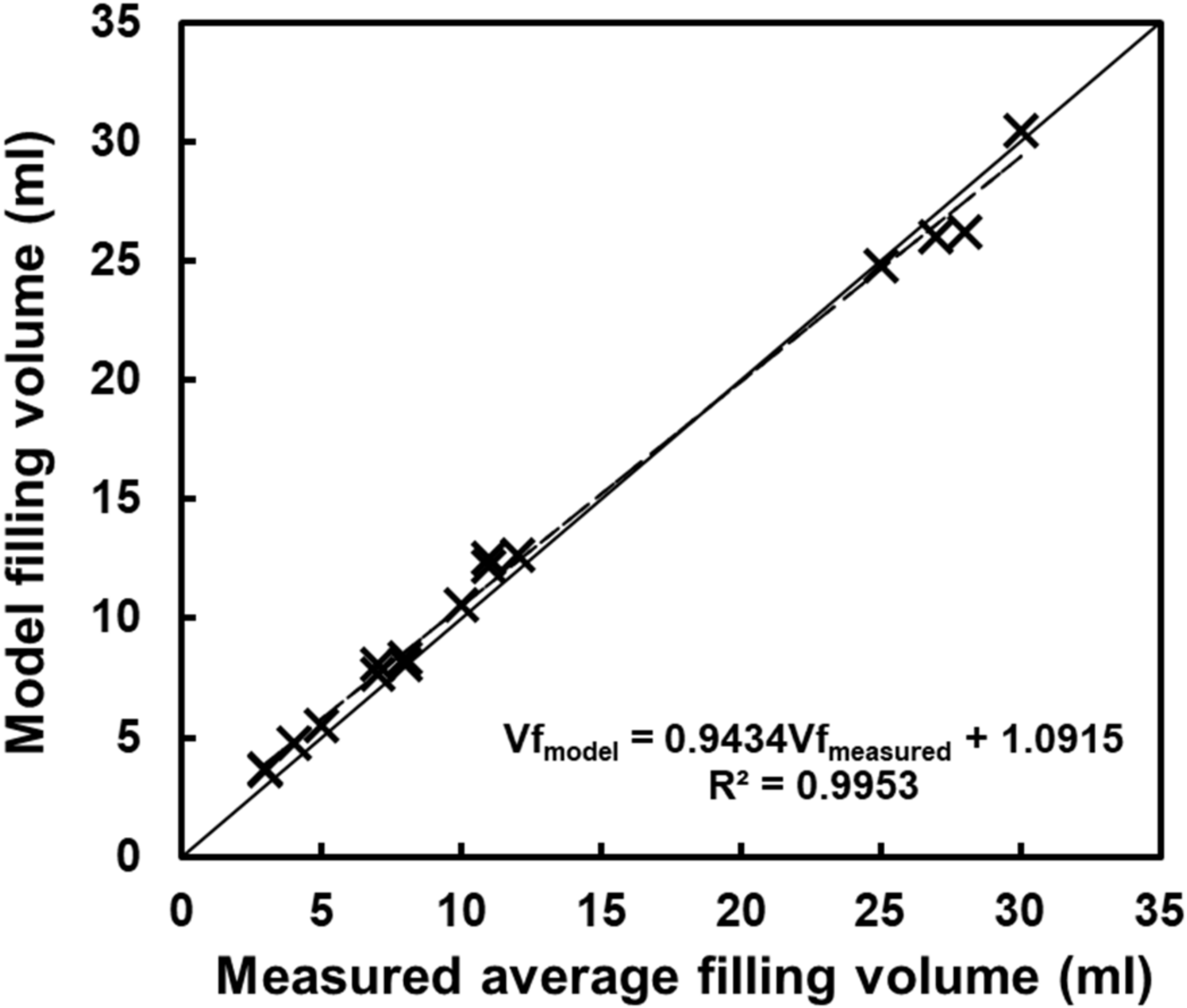
2.4. Validation of the Water Distribution Model
An empirical water distribution model was developed to simulate the flow emitted by each one of the 15,912 emitters for the study irrigation unit. The model was based on the previous characterization of the filling, stable pressure, and emptying phases of the pipe flow process. To validate the water distribution model, four irrigation pulses were applied on four different days in May. The duration of the irrigation pulses was 5, 10, 15, and 20 min. The pressure at the entrance of the irrigation unit was also set at 1 bar in all the irrigation pulses.
To validate the model during the three irrigation phases (filling, stable pressure, and emptying), the water applied by the 60 selected emitters (
Figure 1) was measured. The filling and stable pressure volumes were measured together as a unique stage called the volume of irrigation pulses. The water volumes at the emptying phase were measured separately. The pressure measurement methodology to validate the stable pressure phase was the same used during the characterization stage in the 16 MK measuring points. The values measured were compared to the values predicted by the model.
The water applied by emitters was stored in plastic containers, both from the beginning until the end of the irrigation pulse and from the end of the irrigation pulse until 2 h after the end of the irrigation pulse. Subsequently, the irrigation pulse water volumes were measured using a graduated cylinder of 0.5 l capacity with a 5 mL accuracy.
In the validation stage, 120 plastic containers of 0.7 l were used; 60 of them were used for measuring the volume of irrigation pulse (filling + stable pressure phases), and 60 were used for measuring the water volume of the emptying phase. The water volume was measured using a graduated cylinder of 0.5 l capacity with a 5 mL accuracy.
2.5. Irrigation Performance Indicators
2.5.1. Distribution Uniformity
Distribution uniformity is usually defined as the ratio of the smallest accumulated discharges in the irrigation water distribution to the average discharges of the whole distribution [
29]. The distribution uniformity of the low quarter (UD
lq) is an irrigation performance indicator developed by the United States Department of Agriculture–Natural Resources Conservation Service (USDA-NRCS). UD
lq has been widely accepted by the international irrigation research community for decades [
30,
31], and there is a high correlation between distribution uniformity and other water distribution indicators [
32,
33]. UD
lq is calculated using Equation (5):
where Q
25% is a 25% average flow (l h
−1) with a lower flow of water, Q
avg is the average flow (l h
−1), V
25% is the 25% average water applied volume (l) with a lower volume of water, and V
avg is the average water applied volume (l).
The performance indicator UDlq was calculated both with values measured in the validation stage or with values predicted using the water distribution model generated in this study.
Distribution uniformity in the stable pressure phase (UD
lq_sp) is the water distribution uniformity indicator obtained using classical evaluation methodologies (i.e., Merriam and Keller’s, ASAE’s, and Burt’s). It is important to highlight that UD
lq_sp is independent of the duration of the irrigation pulse. UD
lq_sp was calculated using Equation (3), and Merriam and Keller’s methodology using the following equation:
where Q
25%_sp (l h
−1) is the average flow of 4 MK emitters with a lower water flow during the stable pressure phase, and Q
avg_sp (l h
−1) is the average of the flow of the 16 MK emitters during the stable pressure phase.
The distribution uniformity of the total water applied in the field (UD
lq_field_3phases) depends on the filling, stable pressure, and emptying phases of drip irrigation. UD
lq_field_3phases was calculated for the water volume measured in irrigation pulses of 5, 10, 15, and 20 min in the validation stage. The volume of water applied during these three drip irrigation phases was measured in the 16 MK emitters from the beginning of the irrigation pulse until the emptying of the irrigation system. The duration of the irrigation tests was 2 h of the emptying phase plus the time of the irrigation pulses (5, 10, 15, and 20 min). The UD
lq_field_3phases was calculated using the following equation:
where V
25%_field_3phases (l) is the average of 4 MK emitters with a lower volume of total water applied by the 16 MK emitters from the beginning of the irrigation pulse until the emptying of the irrigation system, and V
avg_field_3phases (l) is the average volume of the 16 MK water volumes measured from the beginning of the irrigation pulse until the emptying of the irrigation system.
The distribution uniformity obtained with the empiric model (UD
lq_model) was calculated for seven simulations of irrigation pulses. Simulations were made every 5 min, from 5 to 30 min, plus an additional simulation of 60 min. The UD
lq_model was calculated using the following equation:
where V
25%_model (l) is the average of 25% with a lower volume of total water applied (including three phases) by 15,912 drip emitters of the irrigation unit, and V
avg_model (l) is the average of the total water applied by the 15,912 drip emitters of the irrigation unit during the three drip irrigation phases.
2.5.2. Potential Application Efficiency for Zero Deficit
Application efficiency provides a general indication of how well an irrigation system performs in delivering water from the irrigation system to the crop. Therefore, application efficiency is a measure of the ratio between the crop water requirements (ET
c) and the total volume of water delivered to the field by the irrigation system (V
water delivered). ET
c was calculated based on FAO methodology, using the measured reference evapotranspiration (ET
o) and local crop coefficients (K
c). ET
o was obtained from a meteorological station belonging to the Agrometeorological Network of Andalusia [
34]. K
c was calculated based on crop coverage using the relationship obtained by [
35].
Potential application efficiency without deficit irrigation at any location (PAE
zerodeficit) occurs when there is no irrigation deficit, and no over-irrigation, at the point where the irrigation water applied was at a minimum. This irrigation performance indicator is especially important for the irrigation strategies of horticultural crops of high added value, such as berries. For these kinds of crops, the farmer’s production strategy is to maximize yield [
14,
35], which requires the absence of water deficit throughout the plot. PAE
zerodeficit can be defined as:
where ne is the number of emitters of the irrigation unit evaluated and V
ETc is the minimum irrigation volume applied by one emitter in the irrigation unit, assuming that the minimum irrigation volume is equal to the crop water requirements.
2.6. Statistical Methods Used to Compare the Model and Data Fit
In order to carry out the subsequent statistical analysis for validating the irrigation distribution model, the following parameters were calculated.
2.6.1. Coefficient of Determination
The coefficient of determination (R2) is a key output of regression analysis. R2 is interpreted as the proportion of the variance in the dependent variable that is predictable from the independent variable. An R2 between 0 and 1 indicates the extent to which the dependent variable is predictable.
2.6.2. Theil’s Inequality Coefficient
Theil’s inequality coefficient (U) was calculated as [
36]:
where Ob
i and Pr
i are the observed (measured) and predicted values and n is the number of data pairs. Parameter U could be 0 or greater. U = 0 means a perfect fit between the model results and observations. A larger U value means a poorer model performance [
36].
2.6.3. Modeling Efficiency
Modeling efficiency (ME) was calculated as [
37]:
where
is the average of predicted values. ME = 1 indicates a perfect fit. ME = 0 reveals that the model is no better than a simple average, and negative values indicate a poor performance.
2.6.4. Standardized Residual
Residual methods calculate the difference between the observed and modelled data points. In our case, the residual plot was a plot of the Standardized Residual (SR) as the dependent variable and the location of the measured points as the descriptor variable [
38]. The standardized residual was calculated as:
4. Discussion
We wanted to know how important it was to include the volume applied during the filling and emptying phases of the pipe flow process on the water distribution and application efficiency without water deficit. Typically, distribution uniformity and application efficiency are calculated assuming constant pressures throughout the irrigation pulse [
23,
24,
25,
39,
40]; however, we hypothesized that it was important to compute the water volume applied during the filling and emptying phases of the pipe flow process for short-duration irrigation pulses, particularly in sloping fields. The study found that the water distribution uniformity and potential application efficiency for zero deficit were greatly affected by the duration of the irrigation pulse for irrigation pulses shorter than 20 min (
Figure 10). The distribution of the volume of water applied during the filling and emptying phases of the pipe flow process contributed decisively to this effect (
Figure 9).
Moreover, the duration of the irrigation pulse has great relevance in sandy soils. In general, short-duration irrigation pulses are associated with lower water loss [
41,
42]. Even in a field experiment, high irrigation frequency led to an equivalent or improved yield and increased water productivity [
8,
43]. Previous studies also indicated the positive role of pulse drip irrigation with increasing the irrigation application efficiency. However, the irrigation events were between 15 and 25 min [
44,
45], which is consistent with the conclusions of this study.
However, it is important to take into account that the quantitative results obtained in this work are conditioned by the type of tapes and emitters of the studied irrigation unit. The used emitter constitutes a particular case of microirrigation systems. In fact, [
46] concluded that the use of pressure-compensating emitters instead of built-in emitters changed the discharge results. In addition, laterals are thin-walled, collapsible polyethylene tapes with built-in emitters. The use of more rigid polyethylene tubes could also change the response of each phase. Despite this constraint, we think the conclusions are sufficiently robust and valid for the purpose of this work. Based on these results, new steps must be taken to generalize the results in any irrigation unit with any kind of irrigation system. Including a rational model in a decision-support tool will help to manage short irrigation pulses under more arbitrary irrigation material, soil, and slope conditions.
The distribution uniformity and potential application efficiency for zero deficit were overestimated for the short irrigation duration if some causes of non-uniformity are ignored. The greater the percentage of volume of water applied during the filling and emptying phases, the worse the performance of the water distribution uniformity and potential application efficiency for zero deficit are (
Figure 9 and
Figure 10). The distribution uniformity value was 93%, which is classified as “excellent” according to Merrian and Keller’s classification, using only stable pressure phase in a 5 min irrigation pulse. However, the value estimated by the water distribution model was 65% when the filling and emptying phases are included, which is classified as “poor” (
Figure 10). Therefore, including the filling and emptying phases has profound practical implications for optimal irrigation scheduling in sloping sandy soils with very short irrigation durations. Optimal irrigation schedules are especially important in sandy soil because sandy soils require a balance in water application efficiency and deep percolation to save water without reducing yields.


